INTRODUCTION TO URBAN WATER DISTRIBUTION - CHAPTER 2 docx
Bạn đang xem bản rút gọn của tài liệu. Xem và tải ngay bản đầy đủ của tài liệu tại đây (1.26 MB, 34 trang )
CHAPTER 2
Water Demand
2.1 TERMINOLOGY
Water conveyance in a water supply system depends on the rates of
production, delivery, consumption and leakage (Figure 2.1).
Water production Water production (Q
wp
) takes place at water treatment facilities. It nor-
mally has a constant rate that depends on the purification capacity of the
treatment installation. The treated water ends up in a clear water reser-
voir from where it is supplied to the system (Reservoir A in Figure 2.1).
Water delivery Water delivery (Q
wd
) starts from the clear water reservoir of the treatment
plant. Supplied directly to the distribution network, the generated flow
will match certain demand patterns. When the distribution area is located
far away from the treatment plant, the water is likely to be transported to
another reservoir (B in Figure 2.1) that is usually constructed at the
beginning of the distribution network. In principle, this delivery is done
at the same constant flow rate that is equal to the water production.
A
Production, Q
wp
Delivery, Q
wd
Demand, Q
d
Consumption, Q
wc
+ Leakage, Q
wl
B
Figure 2.1. Flows in water
supply systems.
© 2006 Taylor & Francis Group, London, UK
Water consumption Water consumption (Q
wc
) is the quantity directly utilised by the
consumers. This generates variable flows in the distribution network
caused by many factors: users’ needs, climate, source capacity etc.
Water leakage Water leakage (Q
wl
) is the amount of water physically lost from the
system. The generated flow rate is in this case more or less constant and
depends on overall conditions in the system.
Water demand In theory, the term water demand (Q
d
) coincides with water consump-
tion. In practice, however, the demand is often monitored at supply
points where the measurements include leakage, as well as the quantities
used to refill the balancing tanks that may exist in the system. In order
to avoid false conclusions, a clear distinction between the measurements
at various points of the system should always be made. It is commonly
agreed that Q
d
ϭ Q
wc
ϩ Q
wl
. Furthermore, when supply is calculated
without having an interim water storage, i.e. water goes directly to the
distribution network: Q
wd
ϭ Q
d
, otherwise: Q
wd
ϭ Q
wp
.
Water demand is commonly expressed in cubic meters per hour
(m
3
/h) or per second (m
3
/s), litres per second (l/s), mega litres per day
(Ml/d) or litres per capita per day (l/c/d or lpcpd). Typical Imperial units
are cubic feet per second (ft
3
/s), gallon per minute (gpm) or mega gallon
per day (mgd).
1
The mean value derived from annual demand records
represents the average demand. Divided by the number of consumers,
the average demand becomes the specific demand (unit consumption per
capita).
Apart from neglecting leakage, the demand figures can often be misin-
terpreted due to lack of information regarding the consumption of vari-
ous categories. Table 2.1 shows the difference in the level of specific
demand depending on what is, or is not, included in the figure. The last
two groups in the table coincide with commercial and domestic water
use, respectively.
Specific demand
Average demand
22 Introduction to Urban Water Distribution
Table 2.1. Water demand in The Netherlands in 2001 (VEWIN).
Annual (10
6
m
3
) Q
d
(l/c/d)
1
Total water delivered by water companies 1247 214
Drinking water delivered by water companies 1177 202
Drinking water paid for by consumers 1119 192
Consumers below 10,000 m
3
/y per connection (metered) 940 161
Consumers below 300 m
3
/y per connection (metered) 714 122
1
Based on total population of approx. 16 million.
1
A general unit conversion table is given in Appendix 7. See also spreadsheet lesson A5.8.1: ‘Flow Conversion’ (Appendix 5).
© 2006 Taylor & Francis Group, London, UK
Accurate forecasting of water demand is crucial whilst analysing the
hydraulic performance of water distribution systems. Numerous factors
affecting the demand are determined from the answers to three basic
questions:
1 For which purpose is the water used? The demand is affected by a
number of consumption categories: domestic, industrial, tourism etc.
2 Who is the user? Water use within the same category may vary due
to different cultures, education, age, climate, religion, technological
process etc.
3 How valuable is the water? The water may be used under circum-
stances that restrict the demand: scarce source (quantity/quality), bad
access (no direct connection, fetching from a distance), low income of
consumers etc.
Answers to the above questions reflect on the quantities and moments
when the water will be used, resulting in a variety of demand patterns.
Analysing or predicting these patterns is not always an easy task.
Uncritical adoption of other experiences where the field information is
lacking is the wrong approach; each case is independent and the conclu-
sions drawn are only valid for local conditions.
Variations in water demand are particularly visible in developing
countries where prosperity is predominantly concentrated in a few major,
usually overcrowded, cities with peripheral areas often having restricted
access to drinking water. These parts of the system will be supplied from
public standpipes, individual wells or tankers, which cause substantial
differences in consumption levels within the same distribution area.
Figure 2.2 shows average specific consumption for a number of large
cities in Asia.
Water Demand 23
0 50 100 150 200 250 300 350
Phnom Penh
Shanghai
Tashkent
Ulaanbaatar
Vientiane
Manila
Kuala Lumpur
Kathmandu
Karachi
Jakarta
Ho Chi Minh City
Dhaka
Delhi
Colombo
Consumption (l/c/d)
Figure 2.2. Specific
consumption in Asian cities
(McIntosh, 2003).
© 2006 Taylor & Francis Group, London, UK
Comparative figures in Africa are generally lower, resulting from the
range of problems that cause intermediate supply, namely long distances,
electricity failures, pipe bursts, polluted ground water in deep wells, etc.
A water demand survey was conducted for the region around Lake
Victoria, covering parts of Uganda, Tanzania and Kenya. The demand
where there is a piped supply (the water is tapped at home) was com-
pared with the demand in un-piped systems (no house connection is
available). The results are shown in Table 2.2.
Unaccounted-for water An unavoidable component of water demand is unaccounted-for water
(UFW), the water that is supplied ‘free of charge’. In quite a lot of trans-
port and distribution systems in developing countries this is the most
significant ‘consumer’ of water, accounting sometimes for over 50% of
the total water delivery.
Causes of UFW differ from case to case. Most often it is a leakage
that appears due to improper maintenance of the network. Other non-
physical losses are related to the water that is supplied and has reached
the taps, but is not registered or paid for (under-reading of water meters,
illegal connections, washing streets, flushing pipes, etc.)
2.2 CONSUMPTION CATEGORIES
2.2.1 Water use by various sectors
Water consumption is initially split into domestic and non-domestic
components. The bulk of non-domestic consumption relates to the water
used for agriculture, occasionally delivered from integral water supply
systems, and for industry and other commercial uses (shops, offices,
schools, hospitals, etc.). The ratio between the domestic and non-domestic
consumption in The Netherlands in the period 1960–2000 is shown in
Figure 2.3.
2
24 Introduction to Urban Water Distribution
Table 2.2. Specific demand around Lake Victoria in Africa (IIED, 2000).
Piped (l/c/d) Un-piped (l/c/d)
Average for the entire region 45 22
Average for urban areas (small towns) 65 26
Average for rural areas 59 8
Part of the region in Uganda 44 19
Part of the region in Tanzania 60 24
Part of the region in Kenya 57 21
2
The domestic consumption in Figure 2.3 is derived from consumers metered below 300 m
3
/y per connection. The real
consumption is assumed to be slightly higher; the figure assessed by VEWIN for 2001 is 126 l/c/d compared to 134 l/c/d in 1995.
© 2006 Taylor & Francis Group, London, UK
In the majority of developing countries, agricultural- and domestic
water consumption is predominant compared to the commercial water
use, as the example in Table 2.3 shows. However, this water is rarely sup-
plied from an integral system.
In warm climates, the water used for irrigation is generally the major
component of total consumption; Figure 2.4 shows an example of some
European countries around the Mediterranean Sea: Spain, Italy and
Greece. On the other hand, highly industrialised countries use huge
quantities of water, often of drinking quality, for cooling; typical exam-
ples are Germany, France and Finland, which all use more than 50%
of the total consumption for this purpose. Striving for more efficient
irrigation methods, industrial processes using alternative sources and
recycling water have been and still are a concern in developed countries
for the last few decades.
2.2.2 Domestic consumption
Domestic water consumption is intended for toilet flushing, bathing and
showering, laundry, dishwashing and other less water intensive or less
frequent purposes: cooking, drinking, gardening, car washing, etc. The
Water Demand 25
1960 1965 1970 1975 1980 1985 1990 1995
Q (l/c/d)
0
50
100
150
200
250
88
35
101
49
97
93
108
95
118
87
122
90
131
106
129
100
2000
129
92
Non-domestic
Domestic
Figure 2.3. Domestic and non-
domestic consumption in The
Netherlands (VEWIN).
Table 2.3. Domestic vs. non-domestic consumption in some African states (SADC,
1999).
Country Agriculture (%) Industry (%) Domestic (%)
Angola 76 10 14
Botswana 48 20 32
Lesotho 56 22 22
Malawi 86 3 10
Mozambique 89 2 9
South Africa 62 21 17
Zambia 77 7 16
Zimbabwe 79 7 14
© 2006 Taylor & Francis Group, London, UK
example in Figure 2.5 shows rather wide variation in the average domestic
consumption of some industrialised countries. Nevertheless, in all the
cases indicated 50–80% of the total consumption appears to be utilised
in bathrooms and toilets.
The habits of different population groups with respect to water use
were studied in The Netherlands (Achttienribbe, 1993). Four factors com-
pared were age, income level, household size and region of the country.
The results are shown in Figure 2.6.
The figures prove that even with detailed statistics available, conclu-
sions about global trends may be difficult. In general, the consumption is
lower in the northern part of the country, which is a less populated, most-
ly agricultural region. Nonetheless, interesting findings from the graphs
are evident: the middle-aged group is the most moderate water user, more
frequent toilet use and less frequent shower use is exercised by older
groups, larger families are with a lower consumption per capita, etc.
26 Introduction to Urban Water Distribution
Agriculture Cooling and others
Urban use Industry
0
20 40
Percentage
60 80 100
Finland
Greece
Germany
Spain
Italy
France
Figure 2.4. Water use in Europe
(EEA, 1999).
Laundry
WC
Bathroom
Other
Dishes
0
20 40
Percentage
60 80 100
Sweden in 1995
Finland in 1998
Denmark in 1995
The Netherlands in 2001
Germany in 2000
189
115
147
126
128
l/c/d
Figure 2.5. Domestic water use
in Europe (EEA, BGW,
VEWIN).
© 2006 Taylor & Francis Group, London, UK
Water Demand 27
Figure 2.6. Structure of domestic consumption in The Netherlands (Achttienribbe, 1993).
© 2006 Taylor & Francis Group, London, UK
In cases where there is an individual connection to the system, the
structure of domestic consumption in water scarce areas may well look
similar but the quantity of water used for particular activities will be
minimised. Apart from the change of habits, this is also a consequence
of low pressures in the system directly affecting the quantities used for
showering, gardening, car washing, etc. On top of this, the water compa-
ny may be forced to ration the supply by introducing regular interrup-
tions. In these situations consumers will normally react by constructing
individual tanks. In urban areas where supply with individual tanks
takes place, the amounts of water available commonly vary between
50–100 l/c/d.
2.2.3 Non-domestic consumption
Non-domestic or commercial water use occurs in industry, agriculture,
institutions and offices, tourism, etc. Each of these categories has its
specific water requirements.
Industry
Water in industry can be used for various purposes: as a part of the final
product, for the maintenance of manufacturing processes (cleaning,
flushing, sterilisation, conveying, cooling, etc) and for the personal
needs (usually comparatively marginal). The total quantities will largely
depend on the type of industry and technological process. They are com-
monly expressed in litres per unit of product or raw material. Table 2.4
gives an indication for a number of industries; an extensive overview can
be found in HR Wallingford (2003).
28 Introduction to Urban Water Distribution
Table 2.4. Industrial water consumption (Adapted from: HR Wallingford, 2003).
Industry Litres per unit product
Carbonated soft drinks
1
1.5–5 per litre
Fruit juices
1
3–15 per litre
Beer
1
4–22 per litre
Wine 1–4 per litre
Fresh meat (red) 1.5–9 per kg
Canned vegetables/fruits 2–27 per kg
Bricks 15–30 per kg
Cement 4 per kg
Polyethylene 2.5–10 per kg
Paper
2
4–35 per kg
Textiles 100–300 per kg
Cars 2500–8000 per car
Notes
1
Largely dependant on the packaging and cleaning of bottles.
2
Recycled paper.
© 2006 Taylor & Francis Group, London, UK
Agriculture
Water consumption in agriculture is mainly determined by irrigation and
livestock needs. In peri-urban or developed rural areas, this demand may
also be supplied from the local distribution system.
The amounts required for irrigation purposes depend on the plant
sort, stage of growth, type of irrigation, soil characteristics, climatic
conditions, etc. These quantities can be assessed either from records or
by simple measurements. A number of methods are available in literature
to calculate the consumption based on meteorological data (Blaney-
Criddle, Penman, etc.). According to Brouwer and Heibloem (1986), the
consumption is unlikely to exceed a monthly mean of 15 mm per day,
which is equivalent to 150 m
3
/d per hectare. Approximate values per
crop are given in Table 2.5.
Water required for livestock depends on the sort and age of the
animal, as well as climatic conditions. Size of the stock and type of
production also play a role. For example, the water consumption for
milking cows is 120–150 l/d per animal, whilst cows typically need only
25 l/d (Brandon, 1984) (see Table 2.6).
Water Demand 29
Table 2.5. Seasonal crop water needs (Brouwer and Heibloem, 1986).
Crop Season Consumption
(days/year) (mm/season)
Bananas 300–365 1200–2200
Beans 75–110 300–500
Cabbages 120–140 350–500
Citrus fruit 240–365 900–1200
Corn 80–180 500–800
Potatoes 105–145 500–700
Rice 90–150 450–750
Sunflowers 125–130 600–1000
Tomatoes 135–180 400–800
Wheat 120–150 450–650
Table 2.6. Animal water consumption (Brandon, 1984).
Animal Litres per day
Cows 25–150
Oxen, horses, etc. 15–40
Pigs 10–30
Sheep, goats 5–6
Turkeys (per 100) 65–70
Chickens (per 100) 25–30
Camels 2–3
© 2006 Taylor & Francis Group, London, UK
Institutions
Commercial consumption in restaurants, shops, schools and other
institutions can be assessed as a total supply divided by the number of
consumers (employees, pupils, patients, etc.). Accurate figures should be
available from local records at water supply companies. Some indica-
tions of unit consumption are given in Table 2.7. These assume individ-
ual connection with indoor water installations and waterborne sanitation,
and are only relevant during working days.
Tourism
Tourist and recreational activities may also have a considerable impact
on water demand. The quantities per person (or per bed) per day vary
enormously depending on the type and category of accommodation; in
luxury hotels, for instance, this demand can go up to 600 l/c/d. Table 2.8
shows average figures in Southwest England.
Miscellaneous groups
Water consumption that does not belong to any of the above-listed
groups can be classified as miscellaneous. These are the quantities used
for fire fighting, public purposes (washing streets, maintaining green
areas, supply for fountains, etc.), maintenance of water and sewage
systems (cleansing, flushing mains) or other specific uses (military facil-
ities, sport complexes, zoos, etc.). Sufficient information on water con-
sumption in such cases should be available from local records.
30 Introduction to Urban Water Distribution
Table 2.7. Water consumption in institutions (adapted from:
HR Wallingford, 2003).
Premises Consumption
Schools 25–75 l/d per pupil
Hospitals 350–500 l/d per bed
Laundries 8
1
–60 litre per kg washing
Small businesses 25 l/d per employee
Retail shops/stores 100–135 l/d per employee
Offices 65 l/d per employee
1
Recycled water used for rinsing
Table 2.8. Tourist water consumption in Southwest
England (Brandon, 1984).
Accommodation Consumption (l/c/d)
Camping sites 68
Unclassified hotels 113
Guest houses 130
1- and 2-star hotels 168
3-, 4- and 5-star hotels 269
© 2006 Taylor & Francis Group, London, UK
Sometimes this demand is unpredictable and can only be estimated on an
empirical or statistical basis. For example, in the case of fire fighting, the
water use is not recorded and measurements are difficult because it is not
known in advance when and where the water will be needed. Provision
for this purpose will be planned with respect to potential risks, which is
a matter discussion between the municipality (fire department) and
water company.
On average, these consumers do not contribute substantially in over-
all demand. Very often they are neither metered nor accounted for and
thus classified as UFW.
PROBLEM 2.1
A water supply company has delivered an annual quantity of
80,000,000 m
3
to a city of 1.2 million inhabitants. Find out the specific
demand in the distribution area. In addition, calculate the domestic
consumption per capita with leakage from the system estimated at
15% of the total supply, and billed non-domestic consumption of
20,000,000 m
3
/y.
Answer:
Gross specific demand can be determined as:
The leakage of 15% of the total supply amounts to an annual loss of
12 million m
3
. Reducing the total figure further for the registered non-
domestic consumption yields the annual domestic consumption of
80Ϫ12Ϫ20 ϭ 48 million m
3
, which is equal to a specific domestic con-
sumption of approx.110 l/c/d.
Self-study:
Workshop problems A1.1.1 and A1.1.2 (Appendix 1)
Spreadsheet lesson A5.8.1 (Appendix 5)
2.3 WATER DEMAND PATTERNS
Each consumption category can be considered not only from the
perspective of its average quantities but also with respect to the timetable
of when the water is used.
Demand variations are commonly described by the peak factors.
These are the ratios between the demand at particular moments and the
average demand for the observed period (hour, day, week, year, etc.). For
example, if the demand registered during a particular hour was 150 m
3
Q
avg
ϭ
80,000,000ϫ1000
1,200,000/365
ഠ183 l/c/d
Water Demand 31
© 2006 Taylor & Francis Group, London, UK
and for the whole day (24 hours) the total demand was 3000 m
3
, the
average hourly demand of 3000/24 ϭ 125 m
3
would be used to determine
the peak factor for the hour, which would be 150/125 ϭ 1.2. Other ways
of peak demand representation are either as a percentage of the total
demand within a particular period (150 m
3
for the above hour is equal to
5% of the total daily demand of 3000 m
3
), or simply as the unit volume
per hour (150 m
3
/h).
Human activities have periodic characteristics and the same applies to
water use. Hence, the average water quantities from the previous para-
graph are just indications of total requirements. Equally relevant for the
design of water supply systems are consumption peaks that appear during
one day, week or year. A combination of these maximum and minimum
demands defines the absolute range of flows that are to be delivered by
the water company.
Time-wise, we can distinguish the instantaneous, daily (diurnal),
weekly and annual (seasonal) pattern in various areas (home, building,
district, town, etc.). The larger the area is, the more diverse the demand
pattern will be as it then represents a combination of several consump-
tion categories, including leakage.
2.3.1 Instantaneous demand
Simultaneous demand Instantaneous demand (in some literature simultaneous demand) is
caused by a small number of consumers during a short period of time: a
few seconds or minutes. Assessing this sort of demand is the starting
point in building-up the demand pattern of any distribution area. On top
of that, the instantaneous demand is directly relevant for network
design in small residential areas (tertiary networks and house
installations). The demand patterns of such areas are much more
unpredictable than the demand patterns generated by larger number of
consumers. The smaller the number of consumers involved, the less
predictable the demand pattern will be.
The following hypothetical example illustrates the relation between
the peak demands and the number of consumers.
A list of typical domestic water activities with provisional unit quan-
tities utilised during a particular period of time is shown in Table 2.9.
Parameter Q
ins
in the table represents the average flow obtained by divid-
ing the total quantity with the duration of the activity, converted into
litres per hour.
Instantaneous flow For example, activity ‘A–Toilet flushing’ is in fact refilling of the
toilet cistern. In this case there is a volume of 8 l, within say one
minute after the toilet has been flushed. In theory, to be able to fulfil this
requirement, the pipe that supplies the cistern should allow the flow of
8 ϫ 60 ϭ 480 l/h within one minute. This flow is thus needed within a
32 Introduction to Urban Water Distribution
© 2006 Taylor & Francis Group, London, UK
relatively short period of time and is therefore called the instantaneous
flow.
Although the exact moment of water use is normally unpredictable,
it is well known that there are some periods of the day when it happens
more frequently. For most people this is in the morning after they wake-
up, in the afternoon when they return from work or school or in the
evening before they go to sleep.
Considering a single housing unit, it is not reasonable to assume a
situation in which all water-related activities from the above table are exe-
cuted simultaneously. For example, in the morning, a combination of activ-
ities A, B, D and H might be possible. If this is the assumed maximum
demand during the day, the maximum instantaneous flow equals the sum
of the flows for these four activities. Hence, the pipe that provides water
for the house has to be sufficiently large to convey the flow of:
Instantaneous peak factor With an assumed specific consumption of 120 l/c/d and, say, four people
living together, the instantaneous peak factor will be:
Thus, there was at least one short moment within 24 hours when the
instantaneous flow to the house was 73 times higher than the average
flow of the day.
Applying the same logic for an apartment building, one can assume
that all tenants use the water there in a similar way and at a similar
moment, but never in exactly the same way and at exactly the same
moment. Again, the maximum demand of the building occurs in the
pf
ins
ϭ
1460
120 ϫ 4/24
ϭ 73
480 ϩ 500 ϩ 180 ϩ 300 ϭ 1460
1/h
Water Demand 33
Table 2.9. Example of domestic unit water consumption.
Activity Total quantity Duration Q
ins
(litres) (minutes) (l/h)
A – Toilet flushing 8 1 480
B – Showering 50 6 500
C – Hand washing 2 1/2 240
D – Face and teeth 3 1 180
E – Laundry 60 6 600
F – Cooking 15 5 180
G – Dishes 40 6 400
H – Drinking 1/4 1/20 300
I – Other 5 2 150
© 2006 Taylor & Francis Group, London, UK
morning. This could consist of, for example, toilet flushing in say three
apartments, hand washing in two, teeth brushing in six, doing the laun-
dry in two and drinking water in one. The maximum instantaneous flow
out of such a consumption scenario case would be:
which is the capacity that has to be provided by the pipe that supplies the
building. Assuming the same specific demand of 120 l/c/d and for pos-
sibly 40 occupants, the instantaneous peak factor is:
Any further increase in the number of consumers will cause the further
lowering of the instantaneous peak factor, up to a level where this factor
becomes independent from the growth in the number of consumers. As
a consequence, some large diameter pipes that have to convey water for
possibly 100,000 consumers would probably be designed based on a
rather low instantaneous peak factor, which in this example could be 1.4.
Simultaneity diagram A simultaneity diagram can be obtained by plotting the instantaneous
peak factors against the corresponding number of consumers. The three
points from the above example, interpolated exponentially, will yield the
graph shown in Figure 2.7.
In practice, the simultaneity diagrams are determined from a field
study for each particular area (town, region or country). Sometimes, a
good approximation is achieved by applying mathematical formulae; the
equation: pf
ins
≈ 126 ϫ e
(Ϫ0.9 ϫ logN)
where N represents the number of con-
sumers, describes the curve in Figure 2.7. Furthermore, the simultaneous
pf
ins
ϭ
6000
120ϫ40/24
ϭ 30
3A ϩ 3B ϩ 2C ϩ 6D ϩ 2E ϩ 1H ϭ 6000
l/h
34 Introduction to Urban Water Distribution
1 10
0
10
20
30
40
50
60
70
73
30
1.40
80
100
Number of consumers
Maximum peak factor
1000 10,000 100,000 1,000,000
Figure 2.7. Simultaneity
diagram (example).
© 2006 Taylor & Francis Group, London, UK
curves can be diversified based on various standards of living i.e. type of
accommodation, as Figure 2.8 shows.
In most cases, the demand patterns of more than a few thousand peo-
ple are fairly predictable. This eventually leads to the conclusion that the
water demand of larger group of consumers will, in principle, be evenly
spread over a period of time that is longer than a few seconds or minutes.
This is illustrated in the 24-hour demand diagram shown in Figure 2.9
for the northern part of Amsterdam. In this example there were nearly
130,000 consumers, and the measurements were executed at 1-minute
intervals.
Hourly peak factor One-hour durations are commonly accepted for practical purposes and
the instantaneous peak factor within this period of time will be repre-
sented by a single value called the hourly (or diurnal) peak factor, as
shown in Figure 2.10.
Water Demand 35
Luxury
Medium
Low
1 1000
0
5
10
15
20
25
30
35
40
45
50
55
60
Number of inhabitants
Maximum peak factor
10,000 100,000
Figure 2.8. Simultaneity
diagram of various categories of
accommodation.
0 6 12
Hours
Peak factors
18 24
0.0
0.2
0.4
0.6
0.8
1.0
1.2
1.4
1.6
1.8
2.0
Figure 2.9. Demand pattern in
Amsterdam (Municipal Water
Company Amsterdam, 2002).
© 2006 Taylor & Francis Group, London, UK
There are however extraordinary situations when the instantaneous
demand may substantially influence the demand pattern, even in the case
of large numbers of consumers.
Figures 2.11 and 2.12 show the demand pattern (in m
3
/min) during
the TV broadcasting of two football matches when the Dutch national
team played against Saudi Arabia and Belgium at the 1994 World Cup in
the United States of America. The demand was observed in a distribution
area of approximately 135,000 people.
The excitement of the viewers is clearly confirmed through the
increased water use during the break and at the end of the game, despite
the fact that the first match was played in the middle of the night (with
different time zones between The Netherlands and USA). Both graphs
point almost precisely to the start of the TV broadcast that happened at
01:50 and 18:50, respectively. The water demand dropped soon after the
start of the game until the half time when the first peak occurs; it is not
difficult to guess for what purpose the water was used! The upper curves
36 Introduction to Urban Water Distribution
0 6 12
Hours
Peak factors
18 24
0.0
0.2
0.4
0.6
0.8
1.0
1.2
1.4
1.6
1.8
2.0
Figure 2.10. Instantaneous
demand from Figure 2.9
averaged by the hourly peak
factors.
0 1 2 3 4 5 6 7 8
0
10
20
30
Q(m
3
/min) Q(m
3
/min)
Hours
Tuesday, 21 June The Netherlands-Saudi Arabia
Start TV broadcast
0 1 2 3 4 5 6 7 8
0
10
20
30
Tuesday, 14 June
Figure 2.11. Night-time
demand during football game
(Water Company
‘N-W Brabant’, NL, 1994).
© 2006 Taylor & Francis Group, London, UK
in both figures show the demand under normal conditions, one week
before the game at the same period of the day.
This phenomenon is not only typical in The Netherlands; it will be
met virtually everywhere where football is sufficiently popular. Its con-
sequence is a temporary drop of pressure in the system while in the most
extreme situations a pump failure might occur. Nevertheless, these
demand peaks are rarely considered as design parameters and adjusting
operational settings of the pumps can easily solve this problem.
PROBLEM 2.2
In a residential area of 10,000 inhabitants, the specific water demand is esti-
mated at 100 l/c/d (leakage included). During a football game shown on the
local TV station, the water meter in the area registered the maximum flow
of 24 l/s, which was 60% above the regular use for that period of the day.
What was the instantaneous peak factor in that case? What would be the
regular peak factor on a day without a televised football broadcast?
Answers:
In order to calculate the peak factors, the average demand in the area has
to be brought to the same units as the peak flows. Thus, the average flow
becomes:
The regular peak flow at a particular point of the day is 60% lower than
the one registered during the football game, which is 24/1.6 ϭ 15 l/s.
Q
avg
ϭ
10,000 ϫ 100
24/3600
ഠ12 l/s
Water Demand 37
0
10
20
30
40
0
10
20
30
40
Hours
Saturday, 25 June The Netherlands-Belgium
16
17 18 19 20 21 22 23 24
16 17 18 19 20 21 22 23 24
Saturday, 18 June
Q(m
3
/min)Q(m
3
/min)
Start TV broadcast
Figure 2.12. Evening demand
during football game (Water
Company ‘N-W Brabant’, NL,
1994).
© 2006 Taylor & Francis Group, London, UK
Finally, the corresponding peak factors will be 24/12 ϭ 2 during the
football game, and 15/12 ϭ 1.25 in normal supply situations.
Self-study:
Workshop problems A1.1.3–A1.1.5 (Appendix 1)
2.3.2 Diurnal patterns
Diurnal demand diagram For sufficiently large group of consumers, the instantaneous demand
pattern for 24-hour period converts into a diurnal (daily) demand
diagram. Diurnal diagrams are important for the design of primary and
secondary networks, and in particular their reservoirs and pumping
stations. Being the shortest cycle of water use, a one-day period implies
a synchronised operation of the system components with similar supply
conditions occurring every 24 hours.
The demand patterns are usually registered by monitoring flows at
delivery points (treatment plants) or points in the network (pressure
boosting stations, reservoirs, control points with either permanent or
temporary measuring equipment). With properly organised measure-
ments the patterns can also be observed at the consumers’ premises.
First, such an approach allows the separation of various consumption
categories and second, the leakage in the distribution system will be
excluded, resulting in a genuine consumption pattern.
A few examples of diagrams for different daily demand categories
are given in Figures 2.13–2.16.
A flat daily demand pattern reflects the combination of impacts from
the following factors:
– large distribution area,
– high industrial demand,
– high leakage level,
– scarce supply (individual storage).
38 Introduction to Urban Water Distribution
Hodaidah
0 4 8 12
Hours
Hourly peak factors
16 20 24
0.0
0.5
1.0
1.5
2.0
2.5
Zadar
Figure 2.13. Urban demand
pattern (adapted from: Gabri-,
1996 and Trifunovi-, 1993).
© 2006 Taylor & Francis Group, London, UK
Commonly, the structure of the demand pattern in urban areas looks as
shown in Figure 2.17: the domestic category will have the most visible
variation of consumption throughout the day, industry and institutions
will usually work in daily shifts, and the remaining categories, including
leakage, are practically constant.
Water Demand 39
Brewery
0 4 8 12
Hours
Hourly peak factors
16 20 24
0.0
0.2
0.4
0.6
0.8
1.0
1.2
1.4
1.6
Aluminium
p
roduction
Figure 2.14. Industrial demand
pattern – example from Bosnia
and Herzegovina (Obradovi-,
1991).
Nightclub
0 4 8 12
Hours
Hourly peak factors
16 20 24
0.0
Hotel
0.2
0.4
0.6
0.8
1.0
1.2
1.4
1.6
1.8
2.0
Figure 2.15. Tourist demand
pattern – example from Croatia
(Obradovi-, 1991).
Hospital
0 4 8 12
Hours
Hourly peak factors
16 20 24
0.0
Commercial
0.2
0.4
0.6
0.8
1.0
1.2
1.4
1.6
1.8
2.0
Figure 2.16. Commercial/
institutional demand pattern –
example from USA (Obradovi-,
1991).
© 2006 Taylor & Francis Group, London, UK
By separating the categories, the graph will look like Figure 2.18,
with peak factors calculated for the domestic consumption only, then for
the total consumption (excluding leakage), and finally for the total
demand (consumption plus leakage). It clearly shows that contributions
from the industrial consumption and leakage flatten the patterns.
2.3.3 Periodic variations
The peak factors from diurnal diagrams are derived on the basis of
average consumption during 24 hours. This average is subject to two
additional cycles: weekly and annual.
Weekly demand pattern Weekly demand pattern is influenced by average consumption on working
and non-working days. Public holidays, sport events, etc. play a role in this
case as well. One example of the demand variations during a week is shown
in Figure 2.19. The difference between the two curves in this diagram
reflects the successful implementation of the leak detection programme.
Consumption in urban areas of Western Europe is normally lower over
weekends. On Saturdays and Sundays people rest, which may differ in
40 Introduction to Urban Water Distribution
Industry
0 4 8 12
Hours
Q (l/s)
16 20 24
0
Domestic
500
1000
1500
2000
2500
3000
3500
4000
4500
Leakage
Other
Figure 2.17. Typical structure
of diurnal demand in urban
areas.
Domestic consumption
0 4 8 12
Hours
Hourly peak factors
16 20 24
0.0
Delivery
Consumption
0.2
0.4
0.6
0.8
1.0
1.2
1.4
1.6
1.8
2.0
Figure 2.18. Peak factor
diagrams of various categories
from Figure 2.17.
© 2006 Taylor & Francis Group, London, UK
other parts of the world. For instance, Friday is a non-working day in
Islamic countries and domestic consumption usually increases then.
Seasonal variations Annual variations in water use are predominantly linked to the change of
seasons and are therefore also called seasonal variations.
The unit consumption per capita normally grows during hot seasons
but the increase in total demand may also result from a temporarily
increased number of consumers, which is typical for holiday resorts.
Figure 2.20 shows the annual pattern in Istria, Croatia on the Adriatic
coast; the peaks of the tourist season, during July and August, are also
the peaks in water use.
Just as with diurnal patterns, typical weekly and annual patterns can
also be expressed through peak factor diagrams. Figure 2.21 shows an
example in which the peak daily demand appears typically on Mondays
and is 14% above the average, while the minimum on Sundays is 14%
below the average daily demand for the week. The second curve shows
the difference in demand between summer and winter months, fluctuat-
ing within a margin of 10%.
Generalising such trends leads to the conclusion that the absolute peak
consumption during one year occurs on a day of the week, and in the
month when the consumption is statistically the highest. This day is com-
monly called the maximum consumption day. In the above example, the
Maximum consumption
day
Water Demand 41
Mon Tue Wed Thu
Q (l/s)
Fri Sat Sun
20
40
60
80
100
120
140
160
180
Peak week 1988
Peak week 1990
Figure 2.19. Weekly demand
variations – Alvington, UK
(Dovey and Rogers, 1993).
Jan
Monthly peak factors
0
0.5
1.0
1.5
2.0
2.5
Feb
Mar Apr May June July Aug Sep Oct Nov Dec
Figure 2.20. Seasonal demand
variation in a sea resort
(Obradovi-, 1991).
© 2006 Taylor & Francis Group, London, UK
maximum consumption day would be a Monday somewhere in June,
with its consumption being 1.14 ϫ 1.05 ϭ 1.197 times higher than the
average daily consumption for the year. In practice however, the maxi-
mum consumption day in one distribution area will be determined from
the daily demand records of the water company. This is simply the day
when the total registered demand was the highest in a particular year.
Finally, the daily, weekly and annual cycles are never repeated in
exactly the same way. However, for design purposes a sufficient accuracy
is achieved if it is assumed that all water needs are satisfied in a similar
schedule during one day, week or year. Regarding the seasonal varia-
tions, the example in Figure 2.22 confirms this; the annual patterns in the
graph are more or less the same while the average demand grows each
year as a result of population growth.
PROBLEM 2.3
A water supply company delivered an annual quantity of 10,000,000 m
3
,
assuming an average leakage of 20%. On the maximum consumption
day, the registered delivery was as follows:
Hour123456789101112
m
3
989 945 902 727 844 1164 1571 1600 1775 1964 2066 2110
Hour 13 14 15 16 17 18 19 20 21 22 23 24
m
3
1600 1309 1091 945 1062 1455 1745 2139 2110 2037 1746 1018
42 Introduction to Urban Water Distribution
1991 1992 1993 1994 1995 1996
Q (m
3
x 1000/month)
0
200
400
600
800
1000
Figure 2.22. Annual demand
patterns in Ramallah, Palestine
(Thaher, 1998).
Maximum: 1.14 x 1.05= 1.197
Minimum: 0.86 x 0.95= 0.817
0.86
0.95
1.05
1.14
Monday
Tuesday
Wednesday
Thursday
Friday
Saturday
Sunday
January
February
March
April
May
June
July
August
September
October
November
December
Daily peak factors
0.8
0.9
1.0
1.1
1.2
Figure 2.21. Weekly and
monthly peak factor diagrams.
© 2006 Taylor & Francis Group, London, UK
Determine:
a diurnal peak factors for the area,
b the maximum seasonal variation factor,
c diurnal consumption factors.
Answers:
a From the above table, the average consumption on the maximum con-
sumption day was 1454.75 m
3
/h leading to the following hourly peak
factors:
Hour 123456789101112
pf
h
0.680 0.650 0.620 0.500 0.580 0.800 1.080 1.100 1.220 1.350 1.420 1.450
Hour 13 14 15 16 17 18 19 20 21 22 23 24
pf
h
1.100 0.900 0.750 0.650 0.730 1.000 1.200 1.470 1.450 1.400 1.200 0.700
b The average consumption, based on the annual figure, is
10,000,000/365/24 ϭ 1141.55 m
3
/h. The seasonal variation factor is
therefore 1454.75/1141.55 ϭ 1.274.
c The average leakage of 20% assumes an hourly flow of approx.
228 m
3
/h, which is included in the above hourly flows as water loss.
The peak factors for consumption will therefore be recalculated with-
out this figure, as the following table shows:
Hour 123456789101112
m
3
761 717 674 499 616 936 1343 1372 1547 1736 1838 1882
pf
h
0.620 0.584 0.549 0.407 0.502 0.763 1.095 1.118 1.261 1.415 1.498 1.534
Hour 13 14 15 16 17 18 19 20 21 22 23 24
m
3
1372 1081 863 717 834 1227 1517 1911 1882 1809 1518 790
pf
h
1.118 0.881 0.703 0.584 0.680 1.000 1.237 1.558 1.534 1.475 1.237 0.644
The diagram of the hourly peak factors for the two situations will look as
follows:
0 4 8 12
Hours
Hourly peak factors
16 20 24
0.0
Demand
Consumption
0.2
0.4
0.6
0.8
1.0
1.2
1.4
1.6
1.8
2.0
Water Demand 43
© 2006 Taylor & Francis Group, London, UK
Self-study:
Workshop problems A1.1.6 and A1.1.8 (Appendix 1)
Spreadsheet lessons A5.8.2–A5.8.4 (Appendix 5)
2.4 DEMAND CALCULATION
Knowing the daily patterns and periodical variations, the demand flow
can be calculated from the following formula:
(2.1)
The definition of the parameters is as follows: Q
d
is the water demand of
a certain area at a certain moment, Q
wc,avg
the average water consumption
in the area, pf
o
the overall peak factor (this is a combination of the
peak factor values from the daily, weekly and annual diagrams: pf
o
ϭ
pf
h
ϫ pf
d
ϫ pf
m
; the daily and monthly peak factors are normally inte-
grated into one (seasonal) peak factor: pf
s
ϭ pf
d
ϫ pf
m
), l the leakage
expressed as a percentage of the water production and f
c
the unit conversion
factor.
The main advantage of Equation 2.1 is its simplicity although some
inaccuracy will be necessarily introduced. Using this formula, the vol-
ume of leakage increases with higher consumption i.e. the peak factor
value, despite the fixed leakage percentage. For example, if Q
wc,avg
ϭ 1
(regardless of the flow units), pf
o
ϭ 1 and the leakage percentage is 50%,
then as a result Q
d
ϭ 2. Thus, half of the supply is consumed and the
other half is leaked.
If pf
o
ϭ 2, Q
d
ϭ 4. Again, this is ‘fifty-fifty’ but this time the volume of
leakage has grown from 1 to 2, which implies its dependence on the con-
sumption level. This is not true as the leakage level is usually constant
throughout the day, with a slight increase over night when the pressures in
the network are generally higher (already shown in Figure 2.17). Hence, the
leakage level is pressure dependent rather than consumption dependant.
Nonetheless, the above inaccuracy effectively adds safety to the design.
Where this is deemed unnecessary, an alternative approach is suggested,
especially for distribution areas with high leakage percentages:
(2.2)
where:
(2.3)Q
wl
ϭ
l
100
ϫ Q
wp
Q
d
ϭ (Q
wc,avg
ϫpf
o
ϩ Q
wl
)
1
f
c
Q
d
ϭ
Q
wc,avg
ϫ pf
o
(1 Ϫ l/100) ϫ f
c
44 Introduction to Urban Water Distribution
© 2006 Taylor & Francis Group, London, UK
In the case of pf
o
ϭ 1, demand equals production and assuming the same
units for all parameters ( f
c
ϭ 1):
(2.4)
This can be re-written as:
(2.5)
By plugging Equation 2.5 into 2.3 and then to 2.2, the formula for water
demand calculation evolves into its final form:
(2.6)
Where reliable information resulting from individual metering of con-
sumers is not available, the average water consumption, Q
wc,avg
, can be
approximated in several ways:
(2.7)
(2.8)
(2.9)
(2.10)
where n is the number of inhabitants in the distribution area, c coverage
of the area. It can happen that some of the inhabitants are not connected
to the system, or some parts of the area are not inhabited. This factor,
which has a value of between 0 and 1, converts the number of inhabitants
into the number of consumers. q is the specific consumption (l/c/d), d the
population density (number of inhabitants per unit surface area), A the
surface area of the distribution area, q
a
the consumption registered per
unit surface area, n
u
the production capacity (it represents a number of
units (kg, l, pieces, etc.) produced within a certain period), q
u
the water
consumption per unit product.
Unit consumptions, q, q
a
, and q
u
, are elaborated in Paragraph 2.2. The
data for n, c, d, A and n
u
are usually available from statistics or set by
planning: local, urban, regional, etc.
As already mentioned, the demand in large urban areas is often
composed of several consumption categories. More accuracy in the calcu-
lation of demand for water is therefore achieved if the distribution area is
split into a number of sub-areas or districts, with standardised categories
of water users and a range of consumptions based on local experience.
Q
wc,avg
ϭ n
u
q
u
Q
wc,avg
ϭ Acq
a
Q
wc,avg
ϭ dAcq
Q
wc,avg
ϭ ncq
Q
d
ϭ
Q
wc,avg
f
c
ϫ
pf
o
ϩ
l
100 Ϫ l
Q
wp
ϭ
Q
wc,avg
(1 Ϫ l/100)
Q
wp
ϭ Q
wc,avg
ϩ
l
100
ϫ Q
wp
Water Demand 45
© 2006 Taylor & Francis Group, London, UK