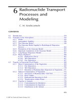
Radionuclide Concentrations in Foor and the Environment - Chapter 6 pot

153

6

Radionuclide Transport
Processes and
Modeling

C. M. Vandecasteele

CONTENTS

6.1 Introduction 154
6.2 Transport in the Atmosphere 155
6.2.1 Winds 155
6.2.2 Atmospheric Stability 156
6.2.3 The Gaussian Model 158
6.2.4 The Gaussian Model Applied to Radiological Dispersion
Devices 162
6.2.5 Parameters of the Gaussian Model 163
6.2.6 Important Limitations of the Gaussian Model 163
6.2.7 Long-Range Dispersion Models 165
6.2.8 Plume Depletion 166
6.2.8.1 Radioactive Decay 167
6.2.8.2 Wet Deposition 167
6.2.8.3 Dry Deposition 167
6.3 Transfer in Terrestrial Food Chains 168
6.3.1 Direct Contamination of the Vegetation 169
6.3.1.1 Dry Deposition 169
6.3.1.2 Wet Deposition 170

6.3.1.3 Retention of Radionuclides Deposited on Vegetation 171
6.3.2 Indirect Contamination of Vegetation 172
6.3.2.1 Interaction of Radionuclides with Soil 172
6.3.2.2 Root Uptake 175
6.3.2.3 Radionuclide Retention in Soil 176
6.3.2.4 Translocation within Plants 177
6.3.3 Transfer to Animals 178
6.3.3.1 Contamination by Inhalation 178
6.3.3.2 Contamination by Ingestion 178
6.3.3.3 Distribution in the Animal 179

DK594X_book.fm Page 153 Tuesday, June 6, 2006 9:53 AM
© 2007 by Taylor & Francis Group, LLC

154

Radionuclide Concentrations in Food and the Environment

6.3.3.4 Excretion 180
6.4 Transport in Aquatic Systems 181
6.4.1 Transport and Dispersion of Radioactivity in Aquatic Systems 182
6.4.1.1 Transport in Rivers 183
6.4.1.2 Transport in Lakes 185
6.4.1.3 Transport in the Marine Environment 186
6.4.1.4 Transport in Estuaries 189
6.4.2 Partition Between the Liquid and Solid Phases 191
6.4.3 Contamination of the Biocenose 192
6.5 Modeling the Transfer of Radionuclides 196
6.5.1 Model Roles and Uses 196
6.5.2 Model Building 196

6.5.2.1 Definition of the Relevant Scenario 197
6.5.2.2 Formulation of the Conceptual Model 197
6.5.2.3 Development of the Mathematical Model 198
6.5.2.4 Estimation of Parameter Values 198
6.5.2.5 Calculation of Model Predictions 199
6.5.3 Uncertainties and Errors Associated with Modeling 199
6.5.4 Model Validation 200
6.5.5 Model Types 200
6.5.5.1 Screening Models 201
6.5.5.2 Emergency Models 201
6.5.5.3 Generic Models 201
6.5.5.4 Experimental Models 201
6.5.5.5 Deterministic and Stochastic Models 202
6.5.5.6 Equilibrium and Dynamic Models 202
6.5.6 Uncertainty Analysis 202
6.5.7 Sensitivity Analysis 204
References 205

6.1 INTRODUCTION

Nuclear electricity production generates large amounts of artificial radionuclides,
which may be concentrated through reprocessing into radioactive wastes. The
many applications of radioactivity in industry, medicine, and research make use
of large quantities of artificial radioisotopes. Finally, some conventional industries
(phosphate mills and oil extraction) concentrate naturally occurring radioactive
materials (NORMs) in their residues. These activities are responsible for routine
and accidental releases of radioactive elements into the environment.
Radionuclides discharged into the atmosphere as gas, aerosols, or fine parti-
cles are transported downwind, dispersed by atmospheric mixing phenomena,
and progressively settled by deposition processes. During the passage of the

radioactive plume, people are irradiated externally as well as internally by inha-
lation. After the passage of the cloud, exposure of the population continues via

DK594X_book.fm Page 154 Tuesday, June 6, 2006 9:53 AM
© 2007 by Taylor & Francis Group, LLC

Radionuclide Transport Processes and Modeling

155

three main pathways: external irradiation from the radionuclides deposited on the
ground, inhalation of resuspended contaminated particles, and ingestion of con-
taminated food products.
When released into surface waters, radionuclides are partly removed from
the water phase by adsorption on suspended solids and bottom sediments. As the
radioactivity disperses, there is a continuing exchange between the liquid and
solid phases. The contaminated sediments deposited on the banks of rivers, lakes,
and coastal areas lead to external irradiation of people spending time at these
sites. The residual activity in water exposes man internally through the ingestion
of drinking water, aquatic food products, and terrestrial food products contami-
nated by irrigation of vegetation and ingestion of water by livestock.
Radioactivity may also contaminate soil due to lixiviation of waste heaps,
shallow land burial, or geological disposal. It migrates slowly with soil water as
soluble ions or organic complexes, interacting with the soil compounds in
exchange reactions, and contaminates aquifers.

6.2 TRANSPORT IN THE ATMOSPHERE

The atmosphere is the first important path for the dispersion of radioactive
pollutants in the environment. Its lower layer, which extends to a height of about

15 km at the equator and 10 km in the polar regions, constitutes the common
receptor of routine industrial gaseous discharges and accidental atmospheric
releases. This layer, called the troposphere, is a turbulent zone, saturated in water
vapor and constantly mixed by winds generated by the heat balance at the Earth’s
surface.

6.2.1 W

INDS

Winds are the driving force for the transport of airborne pollutants. They deter-
mine the direction of the plume of pollutants and the speed at which these
pollutants are transported downwind. Winds are caused by the interaction of the
forces created by the pressure gradients between anticyclones and depressions
and the Coriolis forces generated by the Earth’s rotation. When equilibrium is
reached between these forces, air masses move parallel to the isobars. In the
Northern Hemisphere, the flow is clockwise around high pressure areas and
counterclockwise around depressions.
Closer to the Earth’s surface, however, below 650 m, the shearing forces of
contact with the ground modify wind direction and speed. These friction effects
can cause the wind to change direction by about 30 degrees (outward around
anticyclones and inward around high pressure areas) between altitude (650 m)
and the surface. The forces exerted by the roughness of the ground surface due
to natural (mountains, hills, valleys, forests) and man-made (buildings and cities)
obstacles can change wind trajectories and speed. Variations in wind speed and
direction (along the vertical axis) creates turbulence, which increases the disper-
sion of airborne pollutants.

DK594X_book.fm Page 155 Tuesday, June 6, 2006 9:53 AM
© 2007 by Taylor & Francis Group, LLC

156

Radionuclide Concentrations in Food and the Environment

6.2.2 A

TMOSPHERIC

S

TABILITY

Another key parameter influencing the dispersion of airborne contaminants is the
stability of the atmosphere, which is determined by the vertical temperature profile
of the atmosphere relative to the adiabatic lapse rate, that is, the temperature
decrease that a small air parcel undergoes when rising. As pressure decreases
with height, rising air masses expand and hence cool down. Considering small
air volumes as adiabatic systems (i.e., thermodynamically isolated and not
exchanging energy or heat with their environment), the temperature of a rising
air bubble decreases at a rate of 9.8˚C/km until it becomes water saturated (i.e.,
when water vapor starts to condense). This rate is known as the dry adiabatic
lapse rate. As soon as the air bubble becomes saturated, further rise, and hence
cooling, provoke condensation, which causes its temperature to decrease at a
reduced rate of 6.5˚C/km (termed the saturated or moist adiabatic lapse rate)
because the temperature decrease due to expansion is partially compensated for by
the recovery of the latent vaporization heat released by condensation of water vapor.
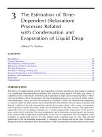
Thus, comparing the actual altitudinal air temperature gradient with the dry
or saturated adiabatic lapse rate (Figure 6.1), the atmosphere is
• Neutral if the actual temperature gradient in the atmosphere is equal

to the adiabatic lapse rate,
• Stable if its temperature gradient is higher than the adiabatic lapse rate,
possibly positive (inversion), and
• Unstable when its temperature gradient is lower than the adiabatic lapse
rate.

FIGURE 6.1

Illustration of the stability conditions of the atmosphere. The dotted arrows
represent the behavior of



an adiabatic air parcel.
Height
T°
stable
unstable
neutral

DK594X_book.fm Page 156 Tuesday, June 6, 2006 9:53 AM
© 2007 by Taylor & Francis Group, LLC

Radionuclide Transport Processes and Modeling

157

The vertical temperature profile in the lower troposphere is directly influence
by
•The thermal fluxes to (insolation in the day time) and from (infrared

radiation during the night) the Earth’s surface,
•The heat capacity of the Earth’s surface (soil or water),
•The thermal conductivity between the Earth’s surface and the lower
air layer in contact, and
•The degree of mixing by winds.
Based on experimental observations, Pasquill [1,2] proposed an empirical
categorization of the stability of the atmosphere in six classes from A (very
unstable) to F (stable), which are based on a few easily observable weather
parameters such as wind speed at 10 m and sunshine intensity in the daytime,
and wind speed and cloud cover during the night (Table 6.1). Later, a class G
was added for very stable atmospheric conditions. The Pasquill stability classi-
fication is still used internationally in atmospheric dispersion modeling.
Using more or less comparable approaches, that is, combining synoptic data
(wind velocity, solar radiation, solar angle, cloudiness), vertical temperature gra-
dient, horizontal fluctuation of the wind direction, and ground surface roughness,
alternative classifications have been proposed by McElroy [3], McElroy and
Pooler [4], Klug [5], Bultynck et al. [6], Vogt [7], and Doury [8], which can be
more or less correlated (Table 6.2).
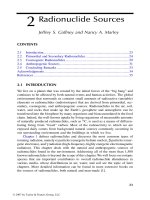
The stability of the atmosphere determines the pattern of the plume (Figure
6.2). The “looping” pattern occurs when the atmosphere is unstable, that is, when
the temperature gradient of the atmosphere is very negative (superadiabatic). This
situation creates whirling air motions that cause the plume to strike the ground
repeatedly along its trajectory. Such conditions (very unstable atmosphere) are
achieved by strong sunshine and weak winds because they require a warm up of
the soil. The “coning” pattern occurs when the atmosphere is neutral or when
the gradient is only slightly superadiabatic (weakly unstable). This situation is

TABLE 6.1
Stability Classes Related to Meteorological Conditions [1]

Wind Speed at
10 m (m/sec)

In the Daytime; Sunshine

During the Night: Cloudiness
Strong Moderate Slight > 3/8

≤

3/8

<2
2–3
3–5
5–6
>6
A
A–B
B
C
C
A–B
B
B–C
C–D
D
B
C
C

D
D
—
E
D
D
D
—
F
E
D
D

DK594X_book.fm Page 157 Tuesday, June 6, 2006 9:53 AM
© 2007 by Taylor & Francis Group, LLC

158

Radionuclide Concentrations in Food and the Environment

the one that is the most faithfully represented by the Gaussian model (see Section
6.2.3). The “fanning” pattern occurs in a stable or very stable atmosphere, when
the gradient is less negative than the adiabatic lapse rate, or even positive.

6.2.3 T

HE

G

AUSSIAN

M

ODEL

The Gaussian model is an empirical model providing an analytical solution to
the transport and diffusion equations representing short duration (puffs) or con-
tinuous (plumes) releases of atmospheric pollutants. It was developed in the early
1960s by Pasquill [1] and Gifford [9], based on a theoretical description of eddy
diffusion in the atmosphere proposed by Sutton [10]. But despite, and also because
of its relative simplicity and because it can be run with limited, readily obtainable
meteorological information, it is still widely used today.

TABLE 6.2
Rough Correspondence of the Stability Classes Between
Different Classification Systems

Pasquill [1] A B C D E F G

McElroy [3]
McElroy and Pooler [4]
B

2

B

1

CD
Bultynck et al. [6]E6E5E4E3–E2E2–E1E1
Doury [8]DNDF

FIGURE 6.2

Typical pollutant dispersion patterns in unstable, neutral, and stable atmo-
spheres. The dotted line on the



left graphs represent the air temperature profile as the
adiabatic lapse rate.
Looping
Coning
T°
T°
h
h
h
unstable
stable
neutral

DK594X_book.fm Page 158 Tuesday, June 6, 2006 9:53 AM
© 2007 by Taylor & Francis Group, LLC

Radionuclide Transport Processes and Modeling

159

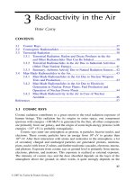
The Gaussian model is based on the assumption that diffusion of airborne
pollutants can be equated to a probabilistic phenomenon, which can be described
by a Gaussian equation. In other words, the concentration profiles in the plane
perpendicular to the wind axis (plume model) as well as on the wind axis (puff
model) adopt Gaussian patterns (Figure 6.3). Therefore the maximum of concen-
tration is centered on the plume axis. The diffusion intensities are expressed by
the values taken by the standard deviations, which increase progressively with
the distance from the source.
In theory, the model applies only for sites with very simple topography (flat
lands, without obstacles or discontinuities) and rather homogeneous meteorolog-
ical conditions during the release and on the puff or plume travel path. Concen-
trations observed at some distance from the release point can have extreme
fluctuations, depending on variations in wind direction and turbulence, therefore
the model provides only average concentrations.
In the case of a puff release, the concentration (

C

(

x

,

y

,

z

,

t

)

) at a given point (

x

,

y

,

z

)
and a given time (

t

) can be estimated by the following mathematical expression:

C

(

x

,

y

,

z

,

t

)

= (6.1)

FIGURE 6.3

Coordinate system for dispersion calculations (after Turner [56]).
z
y
x
h
H
(x,0,0)
(x,y,0)
(x,y,z)
(0,0,0)

QxutyzH
xyz
xy
()
exp
() ()
2
1
2
3
2
2
2
2
2
2
πσσσ
σσσ
−
−
++
−
zz
2




















DK594X_book.fm Page 159 Tuesday, June 6, 2006 9:53 AM
© 2007 by Taylor & Francis Group, LLC

160

Radionuclide Concentrations in Food and the Environment

where

Q

= total quantity of pollutants released at the stack (in kg or Bq),

σ

i

= standard deviations of the Gaussian distribution, representing the
diffusion intensities of the pollutants, along each of the three axes

x

,

y

, and

z

(per m),

u

–

= mean wind velocity at the level of the effective release height

H


(in m/sec),

H

= the so-called effective release height; that is, the actual height of
the stack incremented by an extra height representing the buoyancy

effect (due to initial ejection speed or higher temperature of the
gases released at the stack compared to that of the air) (in m).
For a continuous release (plume), the concentration (

C

(

x

,

y

,

z

)

) at a given point
(

x

,

y

,

z

) is estimated using a similar expression, where the quantity of pollutants
released is replaced by the quotient of the mean emission flux

Φ

(in kg/sec or
Bq/sec) divided by the average wind speed

–

u

(in m/sec). In this case, the diffusion
along the

y

-axis (wind axis), that is, the path of the plume, is neglected because
one may suppose that downstream diffusion is compensated for by upstream
back-diffusion:

C

(

x

,

y

,

z

)

=(6.2)
When the puff or the plume strikes the ground, total reflection is assumed
(i.e., deposition on the ground is not included at this stage). Mathematically this
is achieved by considering a virtual source identical to the actual one, but sym-
metrical relative to the ground surface (Figure 6.4). The pollutant concentrations
in air, beyond the contact point, are the sum of the direct contribution from the
source and that resulting from the pollutants reflection on the ground.
The equations become
(6.3)
for a puff release and
for a plume release.
Φ
u
yzH
yz
yz
2
1
2
2

2
2
2
πσ σ
σσ
exp
()
− +
−


















.
C
Qxuty

xyz
xyz
xy
(,,)
()
exp
()
= −
−
+
2
1
2
3
2
2
2
2
πσσσ
σσ
22
2
2
1
2



















×
−
−




exp
()zH
z
σ


+ −
+

















exp
()1
2
2
2
zH
z
σ
C
u
y
xyz
yz
y
(,,)
exp exp= −









× −
Φ
2
1
2
1
2
2
2
πσ σ
σ
(()
exp
()zH zH
zz
−







+ −
+











2
2
2
2
1
2
σσ





(6.4)

DK594X_book.fm Page 160 Tuesday, June 6, 2006 9:53 AM
© 2007 by Taylor & Francis Group, LLC

Radionuclide Transport Processes and Modeling

161

Similar constructions can be made to cope with temperature inversions
(Figure 6.5), through which the penetration of pollutants is not supposed to
happen. For example, when the inversion is higher than the effective release, a
virtual source of emission must be created at a height corresponding to the height
of the inversion plus the difference between the inversion height and the effective
release height.

FIGURE 6.4

Schema for coping with the total reflection of the plume on the ground
surface.

FIGURE 6.5

Example of situations when a temperature inversion is observed below or
above the release point.
z
y
x
-H
H
Lofting
Trapping
T°
T°
h

h

DK594X_book.fm Page 161 Tuesday, June 6, 2006 9:53 AM
© 2007 by Taylor & Francis Group, LLC

162

Radionuclide Concentrations in Food and the Environment

6.2.4 T

HE

G

AUSSIAN

M

ODEL

A

PPLIED



TO

R

ADIOLOGICAL


D

ISPERSION

D

EVICES

To cope with recent public and political concerns, the Gaussian model was also
adapted (Figure 6.6) to provide a tool to assess the consequences of the dispersion
of radioactive material by conventional explosives as a consequence of terrorist
actions (“dirty bombs”). Such an application has been developed by the University
of California, Lawrence Livermore National Laboratory [11].
Based on the power of the explosion, related to the amount of explosive
material expressed in weight equivalent of TNT (in kg), the Hotspot model
calculates the height (in meters) of the cloud top (93

×



w

0.25

) and the cloud radius

(

r

= 0.2

×

height of the cloud top). The model then assumes an initial distribution
of the dispersed radioactive material between five initial puffs positioned on top
of each other at different heights from the ground level up to 0.8 times the cloud
top and attributes to each of them a fraction of the total source term (Table 6.3).
With each puff are associated two virtual point sources located at a height
corresponding to that of the puff and at an upwind distance,

d

y

and

d

z

, such that

σ

y

and

σ

z

at the vertical of the explosion epicenter (

x

= 0), for the prevalent
atmospheric stability class, are equal to one-tenth of the cloud top.
For each individual puff, a Gaussian model calculates the concentrations at
any point of coordinates (

x

,

y

,

z

), taking into account possible reflections of the
pollutants on the ground or at the level of an inversion. The expected value is the
sum of the five individual contributions.

FIGURE 6.6

Gaussian model adapted to cope with the dispersion of radioactivity after
the explosion of a radiologic dispersion device (RDD). The picture illustrates the coordi-
nate system for two of the five fractions of the total plume considered by the model.
Redrawn from Hotspot 49 [11].
X
Y
Z
d
y
d
z
H4
eff
H2
eff
H0
eff

DK594X_book.fm Page 162 Tuesday, June 6, 2006 9:53 AM
© 2007 by Taylor & Francis Group, LLC

Radionuclide Transport Processes and Modeling

163

6.2.5 P

ARAMETERS

OF



THE

G

AUSSIAN

M

ODEL

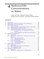
The

σ

values or diffusion coefficients used by the Gaussian model vary according
to the stability of the atmosphere and distance from the source. These values are
provided by approximate formulas (see Brenk et al. [12] and Mayall [13]) or
abacuses (Figure 6.7). It may reasonably be assumed that the diffusion coefficient
along the plume axis,

σ

x

, is similar to

σ

y

.
Measuring the wind velocity at the effective release height (

H

eff

) is not
necessarily directly feasible. It is possible, however, to estimate it based on
measurements at another level (typically at 10 m) according to the following
relation:
(6.5)
where m

ranges from 0.03 to 0.64 according to the stability conditions and the
type of ground surface (Table 6.4).

6.2.6 I

MPORTANT

L

IMITATIONS



OF



THE

G

AUSSIAN
M
ODEL
The application of Gaussian models should, in theory, be limited to environmental
conditions compatible with the assumptions that have been used to derive the
mathematical expressions, namely,
• Constant wind speed (but no calm), wind direction, and air turbulence
along and during the journey of the plume,
• Sufficiently long diffusion times,
• Homogeneous topography and roughness along the plume trajectory, and
•Total reflection of the plume on the ground.
TABLE 6.3
Effective Height and Fraction of the Total
Radioactivity Dispersed Associated with
the Five Individual Puffs
Puff Effective Release Height
Fraction of the
Total Source Term

40.8 × cloud top20%
3 0.6 × cloud top 35%
2 0.4 × cloud top 25%
1 0.2 × cloud top 16%
0 Ground level 4%
uu
H
H
m
eff
eff
10
=






10
DK594X_book.fm Page 163 Tuesday, June 6, 2006 9:53 AM
© 2007 by Taylor & Francis Group, LLC
164 Radionuclide Concentrations in Food and the Environment
FIGURE 6.7 Lateral (
y
) and vertical (
z
) diffusion coefficients as a function of the distance
from the release point. Redrawn based on Pasquill-Gifford approximated equations for a
roughness category 1 [7].

Distance from source (m)
1E+02 1E+03 1E+04 1E+05
1E+00
1E+01
1E+02
1E+03
1E+04
A: very unstable
B: moderatly unstable
C: slightly unstable
D: neutral
E: slightly stable
F: moderatly stable
ECB
F
DA
Distance from source (m)
1E+21E+31E+41E+5
1E+0
1E+1
1E+2
1E+3
1E+4
A
F
E
D
C
B
A: very unstable

B: moderatly unstable
C: slightly unstable
D: neutral
E: slightly stable
F: moderatly stable
σ
Y
σ
z
DK594X_book.fm Page 164 Tuesday, June 6, 2006 9:53 AM
© 2007 by Taylor & Francis Group, LLC
Radionuclide Transport Processes and Modeling 165
These conditions are rarely completely fulfilled in reality, especially over
long distances or long durations. Therefore Gaussian models should only consider
short-range travel. There is wide consensus to consider a range from a few
hundred meters to a few tens of kilometers as valid, however, in practice, modelers
often extend the limit up to 100 km.
The plume occupies a limited space volume, while Gaussian distributions
are, by definition, infinite, therefore estimation is limited to situations where the
calculated concentration values are greater than or equal to one tenth of the
maximal concentration.
6.2.7 LONG-RANGE DISPERSION MODELS
In order to be able to predict plume trajectories over long distances (e.g., the
travel of the Chernobyl clouds over Europe), more complex models have been
developed that call for a much more complete set of meteorological observations
and forecasts from meteorological models (e.g., from the European Centre for
Medium Range Weather Forecasting [ECMWF]), including three-dimensional
wind fields (Figure 6.8).
Eulerian models are based on equations of air mass motion, radionuclide
advection and dispersion, and mass conservation, expressed over a three-dimen-

sional grid, which is fixed with respect to the source origin. Lagrangian models
use a mobile grid that follows the travel of the plume. These two model families
have their respective advantages and drawbacks.
Eulerian grid models allow full three-dimensional development of pollutant
transport, but need more computation time. They are very high-performance tools
to cope with atmospheric pollutant chemistry and transformation. They are unable
to assess the short-range impact of multiple individual sources, especially when
the emission sources do not belong to distinct grid cells. This limitation arises
because these models uniformly mix the emissions within the source grid cell,
and hence do not properly address the initial growth and dispersion of the
pollutants. This drawback might not be crucial in radioactivity dispersion mod-
eling because releases often originate from a single source.
TABLE 6.4
Values of Parameter m in Relation with the Type
of Ground Surfaces and Pasquill Stability Conditions
in the Atmosphere [14]
Type of Ground Surface
Pasquill Stability Class (cf. Table 6.1)
ABCDEF
Seas and lakes
Agricultural soils
Urban and forest areas
0.03
0.10
0.16
0.05
0.15
0.24
0.06
0.20

0.32
0.08
0.25
0.40
0.10
0.35
0.56
0.12
0.40
0.64
DK594X_book.fm Page 165 Tuesday, June 6, 2006 9:53 AM
© 2007 by Taylor & Francis Group, LLC
166 Radionuclide Concentrations in Food and the Environment
Lagrangian plume and puff models are less demanding. Unlike Eulerian
models, they do well working with a limited number of different sources and
their variation in time. Because they are based on a mobile grid, they are able to
trace the plume from individual sources. They cannot treat chemical processes
unless they are those that can be approximated by first-order kinetics. When
comparisons are made of observed and simulated frequency distributions for fixed
receptors, Lagrangian models provide good estimates of maximum concentration
values, typically within a factor of two or three of those observed. Many models
combine the Lagrangian approach, which follows the history of the release across
a region, with the Eulerian approach for the simulation of pollutant dispersion
through a three-dimensional grid covering that region.
6.2.8 PLUME DEPLETION
As a first stage, most dispersion models estimate the transport of airborne pol-
lutants from their source without considering the processes that reduce the radio-
activity in the air compartment; for example, models consider the total plume
reflection on the ground surface and neglect deposition.
FIGURE 6.8 Example of a long-range plume trajectory. (Courtesy of Dr. L. Van der

Auwera, Royal Meteorological Institute, Brussels, Belgium).
3
2
1
0
−1
−2
4
3
2
1
0
−1
ROYAL METEOROLOGICAL INSTITUTE OF BELGIUM
UNITS = log(Bq h/m
3
)
Time integrated concentration in air
DK594X_book.fm Page 166 Tuesday, June 6, 2006 9:53 AM
© 2007 by Taylor & Francis Group, LLC
Radionuclide Transport Processes and Modeling 167
6.2.8.1 Radioactive Decay
Radioactive decay must be accounted for when dealing with short-lived radio-
isotopes (half-life close to the plume travel duration). The easiest way to perform
this correction is by substituting a modified source term in the previously reported
equations, that is, replacing Q by Q = Q × f
i
, where
or , (6.6)
with λ

i
(per sec) being the radioactive decay constant of radionuclide i. Of course,
the product of the disintegration might not be a stable isotope, so the source term
must also be adapted to take into account the buildup of radioactive daughters.
6.2.8.2 Wet Deposition
Deposition of airborne material onto the ground by the action of precipitation
can be assumed to remove pollutants uniformly throughout the entire air column
up to the top of the plume with first-order kinetics. As for radioactive decay, a
correction factor f
w
can be applied to the source term, that is,
or , (6.7)
where
α
i
= washout coefficient for a radionuclide i (per mm when t is
given in sec),
r = precipitation rate (mm/sec).
Best estimate values of α are 0.58/mm for particulates and 0.40/mm for
elemental iodine. The α values are much less than 0.4/mm for organic iodine and
insignificant for noble gases [14].
6.2.8.3 Dry Deposition
Airborne contaminants can also be removed from the plume in the absence of
precipitation (see Section 6.3.1.1). A correction factor f
D
can be similarly applied
to the source term:
, (6.8)
where v
g

is the dry deposition velocity (m/sec).
fe
i
t
i
=
− ×
()
λ
fe
i
x
u
i
=
− ×






λ
fe
w
rt
i
=
− ××
()

α
fe
w
r
x
u
i
=
− ××






α
fe
D
v
u
e
z
g
h
z
z
z
=
− ×× ×
∂

∫







−








2
2
2
2
0
πσ
σ








DK594X_book.fm Page 167 Tuesday, June 6, 2006 9:53 AM
© 2007 by Taylor & Francis Group, LLC
168 Radionuclide Concentrations in Food and the Environment
Best estimate values of v
g
are 0.002 m/sec for particulates (less than 4 µm) and
0.04 m/sec for elemental iodine. The α values are much less than 0.0002 m/sec
for organic iodine and insignificant for noble gases [14].
6.3 TRANSFER IN TERRESTRIAL FOOD CHAINS
Airborne radionuclides are transported downwind and dispersed by the mixing
processes in the atmosphere. They gradually settle on land surfaces as a result
of different deposition mechanisms. Plants are contaminated by two main pro-
cesses: (1) direct deposition on aerial parts of the standing vegetation and
(2) indirect contamination by root uptake when radionuclides deposited onto the
soil are absorbed by plants along with water and nutrients. In a similar way,
radionuclides present in irrigation water reach plants by direct deposition on aerial
parts (sprinkling) or via the soil by root absorption. Gaseous radioelements like
14
C and
3
H (as water vapor or tritiated hydrogen) penetrate the plants through the
stomata and are incorporated into organic constituents by photosynthesis and
other metabolic processes. Contamination of animals and animal products results
from inhalation and ingestion of contaminated soil particles, feed, and water [15].
The most important pathways of radionuclides in agricultural systems are shown
in Figure 6.9.
During passage of the radioactive cloud, people are irradiated externally as
well as internally by inhalation. Thereafter exposure of the population continues
via three main pathways: external irradiation from the radionuclides deposited

FIGURE 6.9 Main pathways for radionuclides to man in continental agricultural food
chains.
Atmosphere
Wet deposition
Dry deposition
Plant products
Animal products
(milk, meat, eggs)
Excretion
Ingestion
Leaching
Leaching
Root uptake
Irrigation
water
DK594X_book.fm Page 168 Tuesday, June 6, 2006 9:53 AM
© 2007 by Taylor & Francis Group, LLC
Radionuclide Transport Processes and Modeling 169
on the ground, inhalation of resuspended contaminated particles, and ingestion
of contaminated food products.
6.3.1 DIRECT CONTAMINATION OF THE VEGETATION
Direct contamination of the plant aerial parts is the result of two main processes:
dry and wet deposition.
6.3.1.1 Dry Deposition
Dry deposition on the surface of plants aerial parts includes diffusion, impaction,
or sedimentation of radionuclides as vapor or in association with aerosols or solid
particles [16–18]. The interception efficiency of the vegetation depends on several
factors.
The physicochemical characteristics of particles. Studies conducted on
nuclear weapons test sites have shown that particles with a diameter

larger than 45 µm are generally not retained by the vegetation cover but
bounce off the leaves and fall to the ground; smaller particles are more
easily intercepted by the vegetation [19,20]. For very fine particles
(aerosols) or vapor, sedimentation rates are so low that deposition rates
are determined by diffusion processes. Chamberlain [21] showed that
the deposition of very fine particles is inversely proportional to the
thickness of the laminar boundary layer above the leaf surface. The
thickness of this layer is perturbed at the edges of plane surfaces where
most deposition occurs [22].
The density of the vegetation cover. Chadwick and Chamberlain [23]
proposed that the initial interception in grass could be related to the
herbage density. Such an interception model based on the vegetation
biomass [24] is adequate for plants developing a homogeneous canopy
(like pasture grass and cereals in the vegetative growing period) and for
which a good correlation exists between biomass and the leaf area index
(LAI). However, it cannot properly respond to the situation where the
LAI is not a monotonous function of the vegetation biomass, like for
cereals from “shooting” onward. In such cases, an interception model
based on the LAI gives more reliable predictions [25].
The characteristics of the plants. In grass, most of the particles retained
are found on the shoot base below the animal grazing level. Soluble
radionuclides accumulated there can subsequently be remobilized and
redistributed into plant tissues. The inflorescence of cereals has a shape
that favors the interception of fallout particles, which may explain why
wheat was found to be the major source of
90
Sr from weapons testing
fallout in Western diets [26].
The prevailing climatic conditions. Although difficult to account for, the
presence of dew on leaf surfaces favors the capture of falling particles.

DK594X_book.fm Page 169 Tuesday, June 6, 2006 9:53 AM
© 2007 by Taylor & Francis Group, LLC
170 Radionuclide Concentrations in Food and the Environment
The initial interception (D
dry
) of airborne radionuclides by plants due to dry
deposition mechanisms (in Bq/m
2
) can be assessed by
D
dry
= C
air
× v
d
× (1 – e
–µLAI
), (6.9)
where
C
air
= time-integrated activity concentration in the air above the plant
canopy (in Bq/sec/m
3
),
v
d
= deposition velocity characteristic for the radionuclide, its
speciation, and the plant type (in m/sec),
µ = interception coefficient (in kg/m

2
),
LAI = leaf area index (in m
2
/kg) characteristic of the plant species and
its development stage.
6.3.1.2 Wet Deposition
Wet deposition is the process by which soluble radionuclides dissolved in hydrom-
eteors or bound to aerosol and particles are trapped by water drops (rain, snow,
fog, or mist) and deposited on surfaces. Aerosol particles are captured by falling
raindrops below the cloud, termed washout, or incorporated in raindrops within
the cloud where they can serve as condensation nuclei, termed rainout. The
contamination of plants by sprinkling irrigation is similar to wet deposition.
The interception efficiency of the vegetation depends on the size of the
droplets and the amount of rainfall, as well as on changes in radionuclide con-
centrations in the rainwater as a function of the length of the rainfall period. The
foliar surfaces are able to retain a certain quantity of water and the excess water
is leached to the ground. Moreover, if rain lasts, contamination in the atmosphere
is progressively washed out and less-contaminated raindrops reach the plants: the
less-contaminated rainfall will also leach part of the already deposited radioac-
tivity down to the soil.
The initial interception (D
wet
) of airborne radionuclides by plants due to wet
deposition processes (in Bq/m
2
) can be assessed by [27]
D
wet
= × (1 – e

–Λ × t
) ×× (6.10)
where
C
atm
= time-integrated (over the duration of rain) activity concentration in
the atmosphere integrated from the ground level up to the height
of the clouds (in Bq/sec/m
2
),
Λ = scavenging coefficient (per sec),
t = duration of the rain (in sec),
LAI = leaf area index (in m
2
/kg) characteristic of the plant species and its
development stage,
C
t
atm
LAI S××k
r
1−









−
××
×
e
rt
S
ln2
3
,
DK594X_book.fm Page 170 Tuesday, June 6, 2006 9:53 AM
© 2007 by Taylor & Francis Group, LLC
Radionuclide Transport Processes and Modeling 171
S = water storage capacity of the plant surfaces (in mm) characteristic
of the plant type (see Müller and Pröhl [27]),
k = radioelement specific factor,
r = rate of rainfall (in mm/sec).
For high biomass density and low rainfall amounts (drizzle), the water reten-
tion capacity of the plant biomass might not be exceeded and most of the rainwater
will be retained by the vegetation. The expression of the initial interception by
wet deposition becomes
D
wet
= × (1 – e
–Λ × t
). (6.11)
Apart from light rain conditions, wet deposition is likely to be much greater
than dry deposition for aerosols and a few times greater for elemental iodine [28].
Rains are very efficient at driving airborne pollutants toward the ground.
6.3.1.3 Retention of Radionuclides Deposited on Vegetation
Foliar contamination is reduced by radioactive decay, weathering processes (wind,

leaching by rain, fog, dew, mist, or irrigation water), and senescence processes
(shedding of cuticular wax, dieback of old leaves). The activity concentration in
the plant biomass (C
v,t
, in Bq/m
2
) at a given time after the deposit is given by
C
v,t
= × e
–((λ + λw) × t)
, (6.12)
where
Q
v,0
= initial contamination in the vegetation biomass (in Bq/m
2
)
resulting from both dry and wet deposition,
Y
t
= vegetation biomass (in kg/m
2
) at the time of measurement,
λ = radioactive decay constant (per sec),
λ
w
= weathering coefficient (per sec),
t = time elapsed since the deposit (sec).
The radioactivity in plants is also diluted by plant growth and removal of

contaminated parts by harvesting or grazing. The contamination of plants
expressed as the activity concentration may also be approximated in early plant
development stages by
C
v,t
= × e
–((λ + λ
w
+ λ
g
) × t)
, (6.13)
where
Y
0
= vegetation biomass (in kg/m
2
) at the time of the deposit,
λ
g
= dilution coefficient due to plant growth (per sec).
C
t
atm
Q
Y
v
t
,0
Q

Y
v,0
0
DK594X_book.fm Page 171 Tuesday, June 6, 2006 9:53 AM
© 2007 by Taylor & Francis Group, LLC
172 Radionuclide Concentrations in Food and the Environment
Since plant growth depends on the season, λ
g
varies with time. For example,
in the temperate climate of middle Europe, the growth rate of pasture grass varies
from 10 to 2 g/day/m
2
(dry mass) between May and October, resulting in a half-
life on the order of 10 to 50 days [29].
The extent of these processes, excluding physical decay, is estimated by field
loss half-life, also called the “environmental” or “ecological” half-life, which is
the time needed to reduce the contamination level on vegetation by a factor of
two. The combined action of environmental removal processes and physical decay
is termed the effective half-life.
Miller and Hoffman [30] reviewed 25 references reporting ecological half-
life values for various radionuclides, physicochemical forms of the radionuclides,
and plant species. They concluded that ecological half-lives on growing vegetation
for iodine vapor and particles were similar (geometric means of 7.2 and 8.8 days,
respectively) and, in general, half that for particulate forms of other elements.
The ecological half-lives determined on a unit area basis are generally larger than
those calculated on a unit mass basis, as the former do not take into account the
dilution by biomass growth. Hence seasons that affect the vegetation growth rate
play a key role in the field loss parameter on a biomass basis. Hoffman and Baes
[31] suggest that the ecological half-lives for pastures are in general half those
for cereals.

6.3.2 INDIRECT CONTAMINATION OF VEGETATION
Indirect contamination includes the mechanisms that rule the behavior of radio-
nuclides in the soil and the geosphere, their interaction with soil components,
and their uptake by plant roots. These mechanisms depend not only on the
element, but also on soil processes and on the physiological properties of the
plant roots.
6.3.2.1 Interaction of Radionuclides with Soil
Soils are heterogeneous systems combining three immiscible phases (solid, liquid,
and gaseous) in different and changing proportions depending on the humidity
level. Each phase is highly complex and variable in composition and physico-
chemical properties. Soil characteristics and thickness are also highly variable in
space. They are often stratified in layers, termed horizons, lying on parent bed-
rock. The top layer, or topsoil, is rich in organic material, while underlying strata
are essentially inorganic. Inorganic compounds are generally categorized on the
basis of their size: clay (less than 2 µm), silt (2 to 20 µm), sands (20 to 2000 µm),
gravels (2 to 20 mm), and stones (greater than 20 mm).
Soils are dynamic systems; the properties are acquired and modified with
time due to the joint actions of natural factors (variations in temperature and
humidity, erosion) and farming practices. Radionuclides deposited on the ground
or dispersed within the soil are first dissolved in soil water. Dissolving proceeds via
kinetics, depending on the speciation of the radioelement: it is quasi-instantaneous
DK594X_book.fm Page 172 Tuesday, June 6, 2006 9:53 AM
© 2007 by Taylor & Francis Group, LLC
Radionuclide Transport Processes and Modeling 173
for soluble compounds (e.g., CsI), but can be a longer process when radionuclides
are included in insoluble matrices (e.g., fuel particles or vitrified wastes), as
radionuclides cannot be leached before weathering processes in the soil have
altered the matrix [32]. Once in solution, radionuclides can adsorb on the sorption
complex by exchange processes; (co-)precipitate as hydroxides, sulfides, carbon-
ates, or insoluble oxides; form complexes with organic molecules; or remain in

the water phase in an ionic form [33].
One key property of soil is its ability to adsorb ions and to immobilize them
to different extents on the solid phase. Soil colloids (clay minerals and organic
matter) contain a high specific density of negative charges acting as cation
exchange sites. The ability of a soil to adsorb ions is proportional to the density
of exchange sites and is expressed by its cation exchange capacity (CEC, in
mEq/kg). Values reported for the CEC range from 0.3 to 1.5 mEq/kg for kaolinite,
1 to 4 mEq/kg for illite, 8 to 15 mEq/kg for montmorillonite, and 30 to 50 mEq/kg
for organic compounds.
For most ions, adsorption of ions is reversible and equilibrium tends to be
achieved between the concentration in the soil solution and on the sorption
complex. This equilibrium is generally expressed as the distribution coefficient
K
d
(in l/kg), which is the quantity of an element sorbed per unit weight of solids
divided by the quantity of the element dissolved per unit volume of water [34]:
K
d
= (6.14)
where
[ ]
sol.
= activity concentration in the solid phase (in Bq/kg),
[ ]
liq.
= activity concentration in the liquid phase (in Bq/l),
A
sol.
= total radioactivity content in the solid phase (in Bq/kg),
A

liq.
= total radioactivity content in the liquid phase (in Bq/l),
M = solid phase mass (in kg),
V = liquid phase volume (in l),
or dividing the measured activity in each phase by the total activity in the system,
K
d
= (6.15)
where
f
sol.
= fraction of the activity associated with the solid phase
(dimensionless),
f
liq.
= residual fraction of the activity dissolved in the liquid phase
(dimensionless).








=
sol
liq
sol
liq

AM
AV
.
.
.
.
,
/
/
fM
fV
sol
liq
.
.
,
/
/
DK594X_book.fm Page 173 Tuesday, June 6, 2006 9:53 AM
© 2007 by Taylor & Francis Group, LLC
174 Radionuclide Concentrations in Food and the Environment
Reversibility of adsorption is the rule for most chemical ions, but elements
like K
+
and Cs
+
may be trapped and immobilized between the lattices of illite-
type clay minerals. The reversibility of this selective binding is very poor and
the elements bound at these sites can only be removed by alteration of the
crystalline structures due to alternations of drying and rewetting or of freezing

and thawing. Hence the modeling of Cs
+
interactions with clays cannot be fairly
described by a simple K
d
approach and more complex relations must be consid-
ered (see, e.g., Hilton and Comans [35]).
Immobilizing ions by fixation onto the soil solid phase or precipitation delays
or prevents their leaching with percolation water down to below the rooting zone.
However, one should always keep in mind that immobilization might be a tran-
sient process. In other words, if the solid phase can be a sink for radioactivity, it
may become a source according to changes in concentration gradients between
the solid and liquid phases or variations in the soil chemical properties (e.g.,
variation in pH or oxidoreduction potential [E
h
]).
Soluble forms of radionuclides move in surface soils, as in geological layers,
by diffusion and are carried along by the flow of water. A simple way to describe
migration can be derived from the Darcy and Fick laws, taking into account mass
conservation:
+= (6.16)
where
C
s
= activity concentration in the solid phase (in Bq/kg),
C
w
= activity concentration in the solution (Bq/l),
t = time (in sec),
= apparent velocity of the radionuclides along the water flow direction

(m/sec),
= apparent diffusion coefficient (m
2
/sec),
x = travel distance (in m).
The apparent velocity of the radionuclides is related to the Darcy water
velocity v
d
in the soil pores through the equation
= (6.17)
where
θ = soil water content (l/l),
K
d
= distribution coefficient (l/kg),
ρ = soil density (kg/l).
∂
∂
C
t
s
∂
∂
C
t
w
− ×
∂
∂
+×

∂
∂
v
C
x
D
C
x
d
w
app
w
**
,
2
2
v
d
*
D
app
*
v
d
*
v
K
d
d
θρ+×

,
DK594X_book.fm Page 174 Tuesday, June 6, 2006 9:53 AM
© 2007 by Taylor & Francis Group, LLC
Radionuclide Transport Processes and Modeling 175
6.3.2.2 Root Uptake
Roots absorb their nutrients mainly from the soil solution. The solid phase
constitutes a reservoir of nutrients that are made available by the weathering of
minerals, humification of dead organic material, and through exchange reactions
between the solid and liquid phases. The soil solution is thus continuously
depleted of its solutes by root uptake, but it is also continuously replenished from
the soil solid phase.
Due to the complexity and temporal and spatial variability of the soil-plant
system, the uptake of radionuclides from soil is difficult to quantify. The main
physical factors affecting the absorption of nutrients by the roots are
•The chemical properties of ions and ionic interactions, both for adsorp-
tion on soil sorption complexes and for root uptake,
•The ionic concentration in the water solution, which depends on the
quality and quantity of soil colloids (clay minerals and organic matter)
and varies over the course of the growing season according to the
weather (e.g., rainfall increasing the soil moisture) and agricultural
practices (fertilization, liming, manure),
•The pH and E
h
, which affect the solubility of some elements (precip-
itation and dissolution reaction) and strongly influence K
d
values [24].
Because of this complexity and variability, soil-plant transfer is usually quan-
tified empirically by the ratio of the activity concentrations in plants and soil,
termed the transfer factor (B

v
):
B
v
=(6.18)
where
[ ]
plant
= activity concentration in the plant (in Bq/kg dry or fresh weight),
[ ]
soil
= activity concentration in the soil (in Bq/kg dry weight).
By definition, the activity concentration in the soil is averaged over a depth
of 10 cm for pasture grass and over 20 cm for other crop species [36]. The activity
concentration in plants for human consumption is generally related to their fresh
weight, while that in fodders is related to their dry weight.
Immobilizing radionuclides by binding (especially irreversible binding) onto
the soil solid phase or precipitation leads to a progressive reduction of their
biological availability for root uptake and hence a decrease in the soil-plant transfer
factor, which only considers the total activity concentration of the radionuclides
in soil, regardless of whether they are bioavailable or not. This is illustrated by
the set of transfer data obtained in experimental fields artificially contaminated
with
134
CsCl (Figure 6.10). The calculated transfer factors decrease exponentially









plant
soil
,
DK594X_book.fm Page 175 Tuesday, June 6, 2006 9:53 AM
© 2007 by Taylor & Francis Group, LLC
176 Radionuclide Concentrations in Food and the Environment
over 5 years, with a half-life of 8.7 (σ = 1.8) months, before reaching a constant
value corresponding to some 10.4% (σ = 1.4) of the initial availability.
6.3.2.3 Radionuclide Retention in Soil
The disappearance of radionuclides from the plant root zone can be represented
by an exponential decay characterized by an effective removal rate (λ
B
, per sec)
cumulating the effects of three mechanisms:
λ
B
= λ + λ
L
+ λ
Η
, (6.19)
where
λ = radioactive decay constant (per sec),
λ
L
= leaching constant accounting for radionuclide migration out of
the rooting zone (per sec),

λ
H
= removal rate attributable to exportation by harvesting or grazing
(per sec).
Losses by leaching (λ
L
) can be expressed by the ratio
(6.20)
FIGURE 6.10 Changes with time of the transfer factors (B
v
) observed in maize leaves.
01224364860728496108120
Time (months after contamination)
0.0
0.2
0.4
0.6
0.8
1.0
B
v
(kg dw / kg dw)
λ
ρ
θ
L
d
sd
v
dK

=
×+×






*
,
1
DK594X_book.fm Page 176 Tuesday, June 6, 2006 9:53 AM
© 2007 by Taylor & Francis Group, LLC
Radionuclide Transport Processes and Modeling 177
where
= apparent velocity of the radionuclides along the water flow
direction (in m/sec),
d
s
= depth of the rooting zone (in m),
ρ = soil density (in kg/l),
θ = soil water content (dimensionless),
K
d
= distribution coefficient (in l/kg).
Removal associated with plant material exportation from the field (λ
H
) can
be represented by
(6.21)

where
B
v
= soil-plant transfer factor (dimensionless),
M
H
= weight of biomass removed per unit area at each harvest (in kg/m
2
),
N = number of harvests per unit of time (per sec),
ρ = soil density (in kg/l),
d
s
= depth of the rooting zone (in m).
6.3.2.4 Translocation within Plants
Elements absorbed by plants through the root system (indirect contamination) or
through the aerial organs (direct contamination) may be redistributed within
plants. After direct contamination, radioactive elements absorbed by nonroot
absorption processes are redistributed within the plant depending on their mobil-
ity: alkali ions can readily be remobilized, whereas alkaline-earth ions are gen-
erally not redistributed from leaves [37]. Movement of
90
Sr,
144
Ce, and
106
Ru into
the grain of cereals is minimal if deposition takes place in the early stage of
development, while
65

Zn,
55
Fe,
137
Cs,
60
Co, and
54
Mn are more easily translocated
within the plant [38]. Middleton [39] reported that up to 50% of the cesium
deposited on potato leaves may be transferred to tubers, while only 0.01% of the
strontium deposited onto aerial parts migrates to tubers. Similarly, in wheat plants
contaminated before ear emergence, 5% to 10% of the cesium but only 0.1% of
the strontium initially retained by the plant is found in the grain at maturity. When
absorbed from soil, some elements, characterized by very low mobility in plants
(such as zirconium, ruthenium, and plutonium), are retained and accumulated in
the roots and exhibit very low translocation to aerial organs; others (such as
cesium, strontium, and technetium) are more easily translocated and accumulate
preferentially in aerial parts. Consequently the stage of development of the plant
at the time of contamination plays a role in determining the contamination level
of organs that were not present when the contamination occurred [25].
v
d
*
λ
ρ
H
vH
s
BM N

d
=
××
×
,
DK594X_book.fm Page 177 Tuesday, June 6, 2006 9:53 AM
© 2007 by Taylor & Francis Group, LLC