TREATMENT WETLANDS - CHAPTER 7 docx

203
7
Suspended Solids
A major function performed by wetland ecosystems is the
removal of suspended sediments from water moving through
the wetland. These removals are the end result of a compli-
cated set of internal processes, including the production of
transportable solids by wetland biota.
Low water velocities, coupled with the presence of plant
litter (in FWS wetlands) or sand/gravel media (in HSSF and
VF wetlands), promote settling and interception of solid
materials. This transfer of suspended solids from the water to
the wetland sediment bed has important consequences for the
quality of the water, as well as the properties and function of
the wetland ecosystem. Many pollutants are associated with
the incoming suspended matter, such as metals and organic
chemicals, which partition strongly to suspended matter. In
FWS wetlands used for municipal wastewater treatment, the
accretion of solids contributes to a gradual increase in the
bottom elevation of the wetland. However, wetlands used to
treat urban or agricultural stormwater, or those exposed to
periodic ancillary ooding, may have rapid accretions in the
inlet zone.
In HSSF and VF wetlands, incoming suspended matter is
removed primarily through the mechanisms of interception
and settling. Although particle resuspension due to wind,
wave, or animal activity can play an important role in the
sediment cycle of FWS wetlands, these mechanisms are min-
imized in HSSF and VF wetland systems. As a result, par-
ticulate matter tends to accumulate in HSSF and VF wetland
beds, with profound consequences on hydraulic conductivity

and system performance.
It should be noted that the concept of using VF lter
beds to remove incoming total suspended solids (TSS) as the
initial stage of a treatment process dates back to the 1960s.
This concept originated with Dr. Kathe Seidel, and came to
be known as the Max Planck Institute Process (MPIP) or
Krefeld Process (Seidel, 1966; Liénard et al., 1990; Brix,
1994d; Börner et al., 1998). The MPIP system consisted of
batch-fed vertical ow wetland beds followed by HSSF wet-
land stages for further efuent polishing.
7.1 SOLIDS MEASUREMENT
TSS are measured gravimetrically after ltration and dry-
ing (Method 2540D; APHA, 1998), and reported in mg/L.
The organic content is characterized as volatile suspended
solids (VSS), determined from the weight loss on ignition at
550°C. The TSS method has been subjected to considerable
criticism by Gray et al. (2000) for use on “natural” waters,
and these authors recommend a suspended sediment concen-
tration (SSC) analysis as a replacement (Method D 3977.97;
ASTM, 2000). One fundamental difculty is the representa-
tiveness of aliquots, especially if they contain sand particles.
A second difculty is the wide variability of the TSS method
in low concentration ranges. Gray et al. (2000) quote the
Standard Methods precision as a 33% coefcient of variation
at 15 mg/L. TSS measurements are likely to be biased low
compared to SSC measurements.
Turbidity in water is caused primarily by suspended
matter, although soluble colored organic compounds can
contribute. Therefore, turbidity is sometimes used as a sur-
rogate for gravimetric measurement of suspended matter.

The measurement technique involves light scattering. The
instrument is the turbidimeter, consisting of a nephelom-
eter, light source, and photodetector. The standard unit is the
nephelometric turbidity unit (NTU). The correlation between
TSS and NTU is often good for a specic wetland system,
but care must be taken in the extrapolation from one site to
another (Table 7.1). From these results, it may be concluded
that the NTU–TSS relationships for FWS wetland efuents
differ substantially from those for activated sludge efuents,
and vary somewhat between natural systems.
POTENTIAL FOR SAMPLING ERRORS
It is sometimes virtually impossible to sample interior wet-
land waters for TSS because of the disturbance of sediments
caused by sampling. Errors of one to two orders of magni-
tude can easily occur. This is the case in shallow zones of
vegetated FWS wetlands. If the water is deeper than about
20 cm, accurate sampling is possible but not easy. Immer-
sion of a sampler may cause disturbance of bed sediments,
or the currents caused by water rushing into a sample bottle
may disturb those sediments. Ideally, the sample should ow
into the sample bottle at the local velocity of the water in the
wetland. This is termed isokinetic sampling, and is necessary
to prevent extraneous resuspension. It is often not possible to
achieve undisturbed sampling for TSS, and therefore difcult
to obtain proper ow-weighted or volume-weighted values of
TSS at interior points. For this reason, much of the available
TSS data from wetland treatment systems consists of input
and output measurements in pipes and at structures.
This difculty carries over to those chemical constitu-
ents which partition strongly to the solids, or form an integral

part of them. Any interior water sample will likely contain an
unrepresentative proportion of the locally agitatible, or trans-
portable, sediments and particulates. Subsequent analysis for
the total amount of a partitioned or contained substance will
yield an inaccurately high value.
© 2009 by Taylor & Francis Group, LLC
204 Treatment Wetlands
Similar sampling problems exist for HSSF wetlands. Most
of the solids present within a HSSF wetland bed are an accu-
mulation of microbial biolms, intercepted particulate matter,
and plant-root networks. This accumulated material, collec-
tively called a biomat, occurs either as material attached to the
bed media and plant roots or as colloidal material within the
media pores. Because the actual ow velocity, v (see Chapter
2), in an HSSF bed is very low, sampling events can induce
localized ow velocities at the point of sample collection that
are much higher than ambient ow velocities. This disturbs
the in situ biomat and leads to sampling errors.
Introduction of sampling probes within the HSSF bed
disturbs the bed matrix, shearing biomat off bed particles,
which interferes with sample accuracy. As a result, samples
taken within the HSSF bed are typically done using sample
ports fabricated from perforated pipe (the same applies for
VF wetlands). These sample ports are installed during con-
struction and are a permanent feature of the HSSF wetland
bed. Depending on the orientation of the perforated section of
the pipe (horizontal or vertical), these sample ports will pro-
duce a sample that is width-averaged or depth-averaged over
a localized portion of the HSSF wetland bed. A typical HSSF
sample port assembly is shown in Figure 7.1; installation of

the ports within an HSSF wetland is shown in Figure 7.2.
However, the use of such pre-installed internal sampling
ports does not guarantee that samples will be representative,
because solids may still be selectively aspirated into the port.
Difculties in sampling lead to large variability for interior
TSS samples. For instance, the coefcient of variation for
TSS samples from the HSSF bed at Minoa, New York, was
TABLE 7.1
Regressions between Total Suspended Solids and Turbidity for Wetlands, Forced through the Origin
(TSS  0, NTU  0)
NTU/TSS R
2
TSS Range
(mg/L)
Turbidity Range
(NTU) Number Reference
Secondary efuent 0.37–0.50 — — — — Crites and Tchobanoglous (1998)
Secondary efuent 0.42–0.43 — — — — Metcalf and Eddy (1991)
Everglades 0.25 0.80 1–18 0.4–3.4 126 South Florida Water Management District,
unpublished data
River water 0.83 0.77 0–145 0–125 64 Des Plaines River Project, unpublished data
River water 0.66 0.95 50–1,400 100–1,000 23 Harter and Mitsch (2003)
Agricultural runoff 0.75 0.52 — — 1,013 Everglades Nutrient Removal Project,
unpublished data
Submerged vegetation 0.74 0.93 0–215 0–150 >100 James et al. (2002)
Water hyacinths 1.39 0.54 4–18 6–21 12 Crites and Tchobanoglous (1998)
Oxidation pond 0.47 0.06 1–15 1–27 96 Gearheart et al. (1983)
30 cm
4 cm Ø Sch 40 PVC
25 cm

5 cm
3 Rows - 6 mm Ø Holes
(4 Holes per Row)
4 cm Ø PVC Conduit
Spacer (typical)
Stainless steel
band clamp (typical)
10 cm Ø Sch 40 PVC
Gravel layer
Mulch/detritus layer
FIGURE 7.1 Example of a HSSF wetland sampling port. This particular assembly is designed to allow sample collection at three
different bed depths and installation of a thermocouple at the base of the mulch layer.
© 2009 by Taylor & Francis Group, LLC
Suspended Solids 205
72% (N = 534), with no apparent distance proles. Similarly,
the coefcient of variation was 145% (N = 215) in the Grand
Lake, Minnesota, HSSF system.
As a consequence of these sampling difculties, most of
the samples collected in HSSF and VF wetlands consist of
inlet and outlet samples, unless interior sampling ports were
installed in the wetland at the time of construction. Because
of the low ow velocities encountered in these systems, inlet
and outlet works in contact with the water develop a biomat
coating. Again, care must be taken not to disturb this bio-
mat coating. If agitation of the water and sloughing of the
biomat occurs, the sample will be contaminated and is no
longer representative of the wastewater. As a result, high-
energy devices such as dipping buckets and bailers should be
avoided. The use of peristaltic pumps is one preferred sam-
pling method, as the rate of sample withdrawal can be con-

trolled, and the sampling tube can be carefully positioned to
collect a representative sample. Small-diameter guide pipes
are sometimes installed to facilitate placement of the sampler
tubing away from side walls, tank bottoms, and other sources
of sample contamination.
SOLIDS CHARACTERIZATION
The suspended solids entering a treatment wetland may
display widely varying characteristics, according to the
source water involved. Domestic wastewaters at all pretreat-
ment stages contain suspended materials that are primarily
organic. Runoff waters, both urban and agricultural, may
contain high proportions of mineral matter. Other source
waters may involve highly specic characteristics, such as
the colloidal materials that discharge from milking parlors.
The two principal ways of describing solids are: the soil type
and the size distribution.
Soil fractions are often also applied to suspended matter,
especially for situations involving mostly mineral materials.
These fractions are: organic, clay, silt, and sand. The VSS
fraction of the solids is usually taken to be a measure of the
or
ganic fraction (Table 7.2), and the remaining nonvolatile sus-
pended solids (NVSS) are assumed to be the mineral fraction
of the overall TSS. For incoming waters derived from runoff
from mineral soils, the fraction organic may be rather low.
At the Des Plaines site, river water entering averaged 11–16%
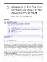
FIGURE 7.2 Four-cell HSSF wetland at the University of Vermont. White pipes extending from the wetland beds are sampling ports.
TABLE 7.2
Organic Content of Various Source Waters Entering Treatment Wetlands
System Influent Source

TSS Inlet
(mg/L) % NVSS
Houghton Lake, Michigan Lagoon 25 56
Estevan, Saskatchewan Lagoon 27 40
Des Plaines, Illinois River 80 24
Tarrant, Texas River 276 10
Tarrant, Texas Sedimentation basin 37 20
Connell, Washington Potato processing 350 94
Note: NVSS = non-volatile suspended solids
© 2009 by Taylor & Francis Group, LLC
206 Treatment Wetlands
organic, whereas water leaving the treatment wetlands aver-
aged 16–26% organic. Harter and Mitsch (2003) reported 9%
organic for both entering and leaving waters from the Olen-
tangy River wetlands. However, the Houghton Lake natural
peatland showed 77% organic, and after lagoon wastewa-
ter addition showed 56% organic (unpublished data). As an
extreme example, the fraction VSS in a potato wastewater
treatment wetland was 94% (unpublished data). Obviously,
no generalizations may be made across the spectrum of
treatment wetlands and source waters, but it should be noted
that organic materials may be subject to decomposition after
deposition.
Mineral constituents may be dened by size ranges
(Lane, 1947; Brix, 1998; Braskerud, 2003):
Clay: size<2µm
Silt: 2 µm < size < 60 µm
Sannd: 60µm <size<2mm
Gravel: 2 mm < size < 64 mm
These mineral particles have relatively high densities, R

s
y
2–2.5 g/cm
3
, and the larger sizes settle readily. In contrast to
organics, these materials accrete without decomposition.
Neither the particles entering the wetland nor those leav-
ing are of a single size. Frequency distributions of particle
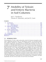
sizes are always present (Figure 7.3). As a result, particle pro-
cessing also becomes distributed, with large particles behav-
ing differently from small.
7.2 PARTICULATE PROCESSES
IN FWS WETLANDS
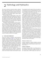
FWS wetlands process sediments and TSS in a number of
ways (Figure 7.4). After the suspended material reaches
the wetland, it joins large amounts of internally generated
suspendable materials, and both are transported across the
wetland. Sedimentation and trapping, and resuspension,
occur en route, as does “generation” of suspended material
by activities both above and below the water surface. For
example, algal debris may form at one location and deposit
downgradient in the wetland.
PARTICULATE SETTLING
Single Particles
The slow-moving waters in the FWS wetland environment often
permit time for physical settling of TSS. The settling velocity of
the incoming particulates, combined with the depth of the wet-
land, gives an estimate of the time and travel distance for those
solids.
Solids sink in water due to the density difference between

the particle and water. For single, isolated spherical particles,
the terminal velocity is reached quickly:
w
gd
C
2
4
3


¤
¦
¥
³
µ
´
D
s
RR
R
(7.1)
where
d
C


particle diameter, m
drag coefficient,
D
ddimensionless

acceleration of gravity, m/g  ss
terminal velocity, m/s
density of wat
2
w 
R eer, kg/m
density of solids, kg/m
3
s
3
R
In turn, the drag coefcient is a function of the particle
Reynolds number:
C
D
p
p

¤
¦
¥
³
µ
´


24
1015
0 687
Re

.Re
.
(7.2)
0.0
0.2
0.4
0.6
0.8
1.0
0 50 100 150 200 250 300
Particle Size (µm)
Fractional Frequency
HL Discharge
HL Background
EW3 In
EW3 Out
FIGURE 7.3 Particle size distributions for two FWS wetlands. At Des Plaines (EW3), the outlet particles are larger than those entering. At
Houghton Lake (HL), the discharge area particles are larger than those in wetland background areas. (From unpublished data.)
© 2009 by Taylor & Francis Group, LLC
Suspended Solids 207
where the particle Reynolds number is:
Re
p

dwR
M
(7.3)
where
Re particle Reynolds number, dimensionless
p


dd 

particle diameter, m
density of water,R kkg/m
terminal velocity, m/s
viscosity o
3
w 
M ff water, kg/m·s (= 0.001µ, in centipoise)
If all physical properties are known, Equations 7.1–7.3 com-
bine to determine the settling velocity. This calculation is
easily automated on a spreadsheet, with the results shown in
Figure 7.5.
In the laminar ow region, Re
p
< 1.0, the drag coef-
cient is inversely proportional to the particle Reynolds num-
ber, and the settling velocity of the particle is then calculable
from Stokes law:
w
gd



2
18M
RR
s
(7.4)

where
d
g


particle diameter, m
acceleration of gravvity, m/s
terminal velocity, m/s
densit
2
w 
R yy of water, kg/m
density of solids, kg/
3
s
R mm
viscosity of water, kg/m·s (= 0.001µ,
3
M iin centipoise)
In the wetland environment, neither the density nor the par-
ticle diameter is known, and the particles are not spheres or
Rainfall & dryfall
particulates
Sedimentation
Inflow Outflow
Periphyton
litterfall
Chemical
precipitation
Plankton &

invertebrate
litterfall
Macrophyte
litterfall
Litter
Resuspension
FIGURE 7.4 Processes affecting particulate matter removal and generation in FWS wetlands. (Adapted from Kadlec and Knight (1996)
Treatment Wetlands. First Edition, CRC Press, Boca Raton, Florida.)
0.0001
0.001
0.01
0.1
1
10
100
1,000
10,000
1 10 100 1,000
Particle Diameter (µm)
Settling Velocity (m/d)
density = 2.00
density = 1.30
density = 1.10
density = 1.03
density = 1.01
Clay Silt Sand
FIGURE 7.5 Settling velocity of spherical particles in water at 20°C, for different particle densities.
© 2009 by Taylor & Francis Group, LLC
208 Treatment Wetlands
discs (Figure 7.6). Although it is possible to correct for non-

spherical shapes (Dietrich, 1982), there is not a convenient
method for determination of the particle density. Further,
particles may agglomerate to larger size, or be subject to
interference from neighboring particles.
Settling of Mixtures
Settling of particulate matter may be described by a rst-order
model (Equation 7.4) for each size fraction. In general, set-
tling velocities are proportional to the square of particle size,
with variation including shape factors and particle density.
Particle mass may be estimated to be roughly proportional to
the cube of size. The time of fall of a particle through a verti-
cal distance (h) is determined from its velocity:
t
h
w
fall

(7.5)
where
h
t
w



water depth, m
time to fall, s
term
fall
iinal velocity, m/s

If the water is moving through the wetland length (L) at
velocity (u), the time of travel is:
t
L
u
travel

(7.6)
where
L
t


wetland length, m
time to traverse
travel
wetland, s
superficial water (flow) velou  ccity, m/s
Theoretically, all particles of a size corresponding to a given
fall velocity will be removed by settling if the travel time
exceeds the settling time from the top of the water:
when
fall
L
u
h
w
N
Lw
uh


1
(7.7)
where
particle falling number, dimensi
fall
N  oonless
These concepts have been applied to mixtures in shallow
overland ow in grass (Deletic, 1999), and in wetlands (Li
et al., 2007), with mean particle diameter used to determine
the settling velocity (w). Values of N
fall
were found to be above
10 for complete removal, reecting the difculty of settling
of the small end of the particle size distribution (Figure 7.7).
These relations also allow the conversion of a size dis-
tribution to a settling velocity distribution, and ultimately to
the size distribution remaining after some xed settling time.
Procedures for such calculations may be found in Crites and
Tchobanoglous (1998); however, there is rarely sufcient
information on particle properties available. Braskerud
(2003) found considerable discrepancies when applying these
procedures to mineral particles trapped in wetlands.
Column Studies
Settling rates may also be determined experimentally. Typi-
cally, a large diameter column of water is charged with a well-
stirred suspension of particles, and the concentration measured
at a sequence of times at a series of depths below the water
surface. Vertical proles of TSS exist in differing shapes,
depending on occulation and particle–particle interference.

A number of analytical techniques may be applied to such data
(Font, 1991). Only the mean water column concentration of
FIGURE 7.6 Photomicrograph of suspended particulate matter
in the efuent from Des Plaines wetland EW3. (From Kadlec and
Knight (1996) Treatment Wetlands. First Edition, CRC Press, Boca
Raton, Florida.)
0.0
0.1
0.2
0.3
0.4
0.5
0.6
0.7
0.8
0.9
1.0
0.01 0.1 1 10 100 1000
Particle Falling Number
Fraction of TSS Trapped
Grass
Wetlands
FIGURE 7.7 Removal of TSS in shallow overland ow in grass.
The particle falling number is (Lw/uh), in which w is the terminal
velocity of the mean particle diameter. Original data centered on a
mean diameter of about 50 µm. (Data from Deletic (1999) Water
Science and Technology 39(9): 129–136; and Li et al. (2007) Jour-
nal of Hydrology 338: 285–296.)
© 2009 by Taylor & Francis Group, LLC
Suspended Solids 209

TSS will be considered here. That concentration decreases as
time progresses. Settling column data, for example, wetland
waters and other sources, indicate an exponential decrease
in concentration with time, and a time scale of a few hours
for the majority of settling to occur (Figure 7.8). The settling
velocities shown in Figure 7.8 range from w = 0.076 to 26.3
m/d. Interestingly, exponential decreases are found for the
several sediments in Figure 7.8.
Caution must be used in those applications where col-
loidal materials may be present in the inow, because these
materials are stable or very slow to settle. Very ne clay
suspensions and some milk processing wastewaters fall into
this category. The settling velocity for planktonic solids was
found to be on the order of w = 0.076 m/d for the Wind Lake,
Wisconsin, wetland, which was dominated by algae.
Column settling data provide estimates of the removal
time for TSS in the absence of dense vegetation. Conrma-
tion of eld applicability was found for wetland EW3 at Des
Plaines in 1991. The inlet zone was essentially unvegetated,
and the water velocity was on the order of 30 m/d. Settling
column data (Figure 7.8) suggested that solids should essen-
tially be gone in eight hours, or after a travel distance of about
ten meters. Transect information conrmed this estimate.
“FILTRATION” VERSUS INTERCEPTION
Conventional wisdom has it that the presence of dense wet-
land vegetation causes settling to be augmented by ltration.
This is often not true in the usual sense of the term ltra-
tion. It is trapping of sediments in the litter layer that prevents
resuspension, and thus enhances the net apparent suspended
sediment removal. Macrophytes and their litter form a non-

homogeneous “ber bed” in the wetland context. The void frac-
tion in the stems and litter is quite high; straining and sieving
are thus not typically the dominant mechanisms. Submerged
biomass additionally traps sediment in sheltered microzones,
thereby lessening the potential for resuspension. Conrmation
of sedimentation as the principal mechanism was provided in
the laboratory studies of Schmid et al. (2005).
However, there are wetland circumstances in which the
dominant mechanism is particles striking immersed objects
and sticking. The three principal mechanisms of ber-bed
ltration are well known and documented in handbooks (see,
e.g., Perry et al., 1982; Metcalf and Eddy, 1991):
1. Inertial deposition or impaction—particles mov-
ing fast enough that they crash head-on into plant
stems rather than being swept around by the water
currents.
2. Diffusional deposition—random processes at
either microscale (Brownian motion) or mac-
roscale (bioturbation) which move a particle to an
immersed surface.
3. Flow-line interception—particles moving with the
water and avoiding head-on collisions, but passing
close enough to graze the stem and its biolm, and
sticking.
The efciencies of collection for these mechanisms depend
on the water velocity, particle properties, and water proper-
ties, as well as the character of submerged surfaces. A typical
wetland “ber” is a bulrush stem of about 1 cm diameter.
Houghton Lake (HL) Discharge
w = 9.6 m/d; R

2
= 0.93
Clay/Alum
w = 26.3 m/d
R
2
= 0.97
10
100
0 100 200 300 400
Time (minutes)
Percent Remaining
Bar El Baqar Clay/Alum
EW3 In EW3 Out
EW5 In EW5 Out
HL Control HL Discharge
EW4 Out Wind Lake
Bar El Baqar
w = 0.076 m/d
R
2
= 0.86
FIGURE 7.8 Examples of settling characteristics of TSS derived from wetlands and other natural contributing sources. The mean settling
velocities range from 0.076 m/d for the Wind Lake wetland TSS, to 26.3 m/d for the clay alum mix. (Data for HL Control, HL Discharge,
EW3 In, EW3 Out, EW4 Out, EW5 In, EW5 Out, and Wind Lake: authors’ unpublished data; data for Clay/Alum: ASCE (1975) Sedimenta-
tion Engineering. Vanoni (Ed.), American Society of Civil Engineers (ASCE): New York; data for Bar El Baqar: PLA (1993) 1993 Field
Program for the Egyptian Engineered Wetland. Report prepared for the United Nations Development Programme, New York, P. Lane and
Associates, Ltd. (PLA).) (Graph from Kadlec and Knight (1996) Treatment Wetlands. First Edition, CRC Press, Boca Raton, Florida.)
© 2009 by Taylor & Francis Group, LLC
210 Treatment Wetlands

A typical particle might be on the order of 1–100 µm. A typi-
cal water velocity is on the order of 10–100 m/d. Under these
conditions, the collection efciencies of Mechanisms 1 and
2 are predicted to be vanishingly small. There is evidence
that Mechanism 3 is operative and signicant. Lloyd (1997)
examined the submerged surfaces of bulrushes (Schoeno-
plectus (Scirpus) validus) and found particles as small as
0.5–2.5 µm sticking to biolms (Breen and Lawrence, 1998).
Saiers et al. (2003) studied the movement of very small (0.3
µm), unsettleable particles of TiO
2
in the Florida Everglades.
They concluded that 29% of the particle impacts on periphy-
ton-coated stems resulted in sticking in a plant (Eleocharis
spp.) density of 1,150 per m
2
. These stems were only 0.2 cm
in diameter, resulting in 99% porosity. Saiers et al. (2003)
dened a rst-order rate constant for removal by sticking,
which on an areal basis is:
k
uh
n
d


§
©
¨
¶

¸
·
H
P
2
2
1
4
(7.8)
where
stem diameter, m
water depth, m
ar
d
h
k


 eeal removal rate constant, m/hr
stem densn  iity, #/m
water velocity, m/hr
sticking
2
u 
H eefficiency, dimensionless
RESUSPENSION
Settled particles may not “stay put” for a number of reasons.
Hydrodynamic shear forces may tear particles loose from the
sediment bed, which is a dominant mechanism in streams and
rivers. However, wetlands provide an environment in which

other processes may occur as well. Wind and wave action
are major drivers of resuspension in lakes, and may also be
operative in open water areas of FWS wetlands. Additionally,
biological activity may result in the movement of particles
from the sediments to overlying water.
Unvegetated Surfaces
Much is known about the resuspension of particulates from
at surfaces (ASCE, 1975). Most interpretations are made
in terms of the force per unit area (shear stress) required to
tear a particle loose from the sediment surface. The concepts
involve purely physical forces and apply most readily to min-
eral substrates and river systems. Most theoretical results are
for planar sediment bed bottoms with no extraneous objects.
Vegetated wetland bottoms do not t these conditions.
In the treatment wetland environment, physical resus-
pension (due to high ow velocities) is not a dominant
process. Water velocities are usually too low to dislodge a
settled particle from either the bottom or a position on sub-
merged vegetation. However, in design, it may be necessary
to avoid wetland aspect ratios that produce excessively high
linear velocities. The potential for erosive velocities exists
for highly loaded wetlands with high length-to-width ratios.
Estimation of the velocity required to foster resuspension
may be based on the settling characteristics of the solids and
the frictional characteristics of the wetland, combined with
known correlations of the critical shear stress for particle
dislodgment (ASCE, 1975). Modications are needed for the
case of laminar ow, which is the general case for wetlands
(Mantz, 1977; Yalin and Karahan, 1979).
Velocities that cause erosion in open channels are high

compared to wetlands. For instance, French (1985) lists rec-
ommended maximum (nonscouring) velocities for 14 canal
materials in the range 0.46 < u < 1.83 m/s. Such consider-
ations resulted in a maximum canal velocity design constraint
of 0.76 m/s for Everglades protection wetlands conveyance
canals (Burns and McDonnell, 1996). In anticipation of more
erodable particulates inside the wetlands, wetland velocities
were limited to no more than 0.03 m/s (2,600 m/d). These
large wetlands had lengths up to 2,500 m, which therefore
c
r
eated a design detention minimum of one day. The annual
average design detention time was 30 days. No erosion has
been noted in this project or its companions of comparable
size and detention.
EffectsofVegetation
It is known that vegetation increases the retention of particu-
lates in both lake and stream environments. For instance, Horp-
pila and Nurminen (2003) found that beds of submerged plant
species—butter cup: Ranunculus circinatus; coontail: Cera-
tophyllum demersum; and pond weed: Potamogeton obtusifo-
lius—in a lake environment effectively prevented resuspension,
which they attributed to a reduction in wind and wave action.
Horvath (2004) studied the effect of macrophytes—rushes: Jun-
cus spp.; bur-reed: Sparganium spp.; forget-me-not: Myosotis
spp.—on retention of particulate matter in a small stream,
and found enhanced trapping in proportion to biomass.
It is logical that these same effects are prevalent in treat-
ment wetlands. Dieter (1990) found about a threefold reduc-
tion in resuspension from open water to vegetated areas in a

prairie pothole wetland. Hosokawa and Horie (1992) demon-
strated enhanced removal in both laboratory channels with
dowels and in eld umes in a reed bed (Phragmites aus-
tralis). In fully vegetated wetlands, the litter and root mats
provide excellent stabilization of the wetland soils and sedi-
ments. This limits, but does not eliminate, resuspension.
The
Floc Layer
Some treatment wetlands, such as those used for low-level
nutrient removal, develop very occulent sediment beds.
These sediments are positioned on top of the consolidated
soils, and may be interwoven with plant detritus. Bulk densi-
ties of such oc layers may range downward to 0.03–0.05
g/cm
3
of dry matter (James et al., 2001; Coveney et al., 2002).
Depths of these loose and unconsolidated materials have
been found to exceed 30 cm in some situations (Table 7.3).
© 2009 by Taylor & Francis Group, LLC
Suspended Solids 211
Despite low bulk density, the amount of oc dry matter is
substantial. For instance, the Sacramento data in Table 7.3
convert to about 9,700 g/m
2
of dry matter present as the oc.
The origins of oc are not well understood, but it has
been found to occur in both macrophyte-dominated (Sac-
ramento) and SAV-dominated (ENRP Cell 4) wetlands. It
likely contains a signicant microbial detrital component, as
well as algal and macrophyte detritus. Floc also occurs in

the ultra-low nutrient, unimpacted Everglades (Gaiser et al.,
2005), where it is presumably the result of an active periphy-
ton biological cycle.
There is not an accepted common terminology for the
oc. Nolte (1997) called it the “A layer,” and described it as
follows:
The A layer consists of a slurry of dark, decomposing, loosely
structured detrital material that pours out when the sam-
pler is tipped. The material in the A layer has settled to the
bottom, but has not been integrated into the matrix of the
basin oor.
This material is not subject to transport under most ambient
conditions, but is very mobile if disturbed. For example, dis-
turbance resuspension tests were conducted at the Houghton
Lake treatment wetland. A bottomless sharp-edged cylinder
was twisted down into the soil, and the interior biomass (live,
dead, litter) was removed. The remaining, isolated water was
gently agitated, and then sampled for solids content. The
mobile material averaged 880 o 100 g/m
2
(mean o SE).
Other Resuspension Mechanisms
The wetland environment provides an opportunity for three
other mechanisms of resuspension: wind-driven turbulence,
bioturbation, and gas lift. In open water areas, wind-driven
currents cause surface ow in the wind direction and return
ows along the bottom in the opposite direction. These recir-
culation velocities can far exceed the net velocity from inlet to
outlet. For wetlands with large open water zones, waves add
to the overall process of resuspension. Lake studies suggest

both processes are wind-dependent. For instance, Malmaeus
and Hakanson (2003) suggest resuspension is proportional to
the square of the wind speed. Additionally, fetch and water
depth are controlling factors.
Animals of all types and sizes can cause resuspension to
occur. Feeding carp (Kadlec and Hey, 1994) and nesting shad
(APAI, 1995) have been observed to cause problems. The
carp rooted in the sediments for food, and thus resuspended
large amounts of sediments. Control was by drawdown and
freezing. The shad fanned nests on the wetland bottom, and
resuspended sediments. Control was by drawdown and avian
predation. Beaver activity can cause stirring, often at the out-
let of the wetland, in conjunction with attempts to dam the
outlet. Human sampling activities in the interior of treatment
wetlands may also result in locally-elevated concentrations
of suspended solids. For instance, the passage of a drifting
boat can cause extreme resuspension (Figure 7.9).
Gas lift occurs when bubbles of gas become trapped in or
attached to particulate matter. Wetland sediments are often
of near neutral buoyancy; so a small amount of trapped gas
can cause “sinkers” to become “oaters.” There are several
gas-generating reactions in a wetland environment. Most
important are photosynthetic production of oxygen by algae
and production of methane in anaerobic zones.
CHEMICAL PRECIPITATES
Several chemical reactions can produce particulate matter
within wetlands under the proper circumstances. Some of
the more important are the oxyhydroxides of iron, calcium
carbonate under aerobic conditions, and divalent metal sul-
des under anaerobic conditions. As conditions of chemical

composition, pH, and redox change in the wetland, these and
other compounds may undergo dissolution and be removed
from the sediment bed.
TABLE 7.3
Floc Thicknesses and Bulk Densities for the Everglades Nutrient Removal Project (ENRP),
Lake Apopka, Florida Project, and the Sacramento California Demonstration Wetlands Project
Thickness (cm) Bulk Density (g/mL)
Site Years Mean SE N Mean SE N
Sacramento 4 2.6 17.2 1.4 8 0.068 0.015 12
Sacramento 4 2.6 11.3 1.0 8 0.069 0.017 16
ENRP 1 9.0 19.7 1.4 30 0.076 0.006 30
ENRP 2 9.0 18.2 1.4 26 0.099 0.007 26
ENRP 3 9.0 18.9 1.8 22 0.072 0.008 22
ENRP 4 9.0 16.7 1.4 10 0.092 0.012 10
Apopka 2.4 33 — 48 0.051 — 48
Source: Data from Nolte and Associates (1997) Sacramento Regional Wastewater Treatment Plant Demonstration Wetlands Project.
1996 Annual Report to Sacramento Regional County Sanitation District, Nolte and Associates: Sacramento, California; Coveney et al.
(2002) Ecological Engineering 19(2): 141–159; and South Florida Water Management District, unpublished data.
© 2009 by Taylor & Francis Group, LLC
212 Treatment Wetlands
Iron Flocs. The iron oxyhydroxides are typically ocs,
with the possibility of coprecipitates. They may form under
conditions of elevated dissolved ferric iron and oxygen-rich
water. The processes may be represented as (Younger et al.,
2002)
Fe O H Fe H O
+
2
2
2

3
1
4
1
2

l
(7.9)
Fe + 2H O FeOOH 3H
2 (sus)
+3
l
(7.10)
FeOOH FeOOH
(sus) (sed)
l
(7.11)
These precipitates are characterized by an unmistakable
blood-red color (Figure 7.10). As indicated by the chemistry,
formation is inhibited by low pH and by low dissolved oxygen.
Formation may be abiotic, or mediated by microorganisms
such as Thiobacillus ferrooxidans. However, at pH > 9, the
rate of the abiotic reaction is so fast that formation is con-
trolled by the rate of oxygen supply (Younger et al., 2002).
In the pH range 6 < pH < 8 that generally typies treatment
wetlands, rates are slow enough to be a design consideration.
This set of reactions forms the basis for phosphorus removal
by addition of ferric chloride to wastewaters, and the accom-
panying co-precipitation of the phosphorus. Consequently,
the subsequent fate of these solids in polishing treatment

wetlands is of considerable interest.
Aluminum Flocs. The aluminum oxyhydroxides are
also typically ocs, with the possibility of co-precipitates.
They may form under circumneutral pH conditions, and do
not require oxygen. The processes may be represented as
(Sobolewski, 1999):
Al H O Al(OH) 3H
3+
23
+
l m
(7.12)
FIGURE 7.9 Passage of a drifting boat can stir up a cloud of oc. This site is in the interior of the A.R. Marshall Loxahatchee National
Wildlife Refuge. The water was about 45 cm deep, and the vegetation was sparse.
FIGURE 7.10 (A color version of this gure follows page 550) Venting groundwater at this Wellsville, New York, site contains iron,
which oxidizes upon contact with air.
© 2009 by Taylor & Francis Group, LLC
Suspended Solids 213
These precipitates are characterized by their formation of a
“pin oc” material that does not readily settle in FWS wet-
lands (Bachand et al., 1999). This set of reactions also forms
the basis for phosphorus removal by addition of alum to
wastewaters, and the accompanying co-precipitation of the
phosphorus. Consequently, the subsequent fate of these solids
in polishing treatment wetlands is of considerable interest.
Calcium Carbonate. Calcium carbonates may be formed
in wetlands, under conditions of elevated pH and dissolved
calcium. The operative chemistry may be summarized as
Ca HCO H O CaCO H
2+

32 3
+
lm

(7.13)
This reaction may occur abiotically, but perhaps more impor-
tantly it may be mediated by algae. Algal activity can drive
up pH, and create conditions that foster creation of calcium-
rich solids (Vymazal, 1995). Indeed, this process has con-
tributed to the formation of marl prairies as a form of natural
wetlands. New sediments in Everglades protection treatment
wetlands contain a signicant fraction of calcium compounds
(Dierberg et al., 2002).
Metal Suldes. Many metals form very insoluble sul-
des, including mercury, lead, cadmium, and zinc, as further
discussed in Chapter 11. These precipitates are important in
the processes of metal removal in wetlands, and follow the
general chemistry (Sobolewski, 1999):
SO HS H HCO
4
2
23
22

lCH O (7.14)
M+HS MS+H
2+ +
l
(7.15)
However, for many treatment wetland applications, metals

are present at only very low concentrations. Consequently,
the formation of insoluble suldes does not usually create
measurable additions to the sediments of the wetlands.
BIOLOGICAL SEDIMENT GENERATION
Wetlands produce sediments via processes of death, litter
fall, and litter attrition. This occurs for biota at a number
of different size scales, ranging from macrophytes on down
to bacteria. Algal productivity can be a major generator of
suspended solids. A second set of processes adds pollen and
seeds to the water. The TSS produced is organic in charac-
ter, resulting in a high carbon content and a high proportion
of VSS. The chlorophyll and pheophytin (dead chlorophyll)
content is high if the algal pathway is dominant.
Some TSS originates from leaf and stem litter. For
instance, annual leaf litterfall in a natural sedge-shrub peat-
land was found to be 60–70 g/m
2
(Chamie, 1976). Some part
of this material contributes to TSS, either via direct attrition,
or via microbial decomposition.
The generation of sedimentary material is a very impor-
tant internal process in nutrient-rich treatment wetlands. The
generous supply of nutrients assures a large production of a
wide variety of transportable organisms and associated dead
organic material. Such wetlands are characterized by high
water chlorophyll content and high sediment accumulation.
Bacterial and algal growth is promoted, and decomposition
products form a new pool of suspendable material. A host of
wetland invertebrates, such as Daphnia and waterboatman
(Corixidae), also die and contribute to the sediments, and

they may be present in pumped lagoon water.
These processes are virtually impossible to predict and
quantify. But it is important to recognize that they exist,
because they contribute to a background level of TSS in a
wetland.
ACCRETION
Trapped TSS, plus material generated within the wetland,
will accrete as either movable sediment or the consolidated
immovable new soil produced from the sediments. Not all
of the dead plant material undergoes decomposition. Some
small portions of both aboveground and belowground nec-
romass resist decay, although these are typically shredded
by microbial and other invertebrate processes. Underground
processes form nonsuspendable accretions, some part of
which is stable and does not fully decompose. The origins of
new sediments may be from remnant macrophyte stem and
leaf debris, remnants of dead roots and rhizomes, and from
indecomposable fractions of dead microora and microfauna
(algae, fungi, invertebrates, bacteria).
Measurement of Accretion
The processes above combine to determine the amount of
sediment at various locations within the wetland as a func-
tion of time and the TSS concentration in the wetland efu-
ent. Cup collectors may be placed on the wetland bottom
(Jordan and Valiela, 1983; Fennessy et al., 1992; Braskerud,
2001a); these typically intercept the downward vertical
ux of sediment but prevent shear-induced resuspension.
Plate collectors may be placed on the wetland bottom, fol-
lowed by sediment harvest above that horizon at a later time
(Kozerski and Leuschner, 1999; Braskerud, 2001a). Alterna-

tively, neutral density particulate material may be laid down
in a layer, and retrieved by coring and sectioning (Harter and
Mitsch, 2003). Another technique involves the elevation of a
blunt-footed rod, which is lowered to the sediment surface.
A reference rod, driven deep into stable soils, provides the
local datum (Reeder, 1990). Other quantitative studies have
relied upon atmospheric deposition markers such as radio-
active cesium (
137
Cs) or radioactive lead (
210
Pb) (Kadlec and
Robbins, 1984; Craft and Richardson, 1993; Robbins et al.,
2004). These techniques require several years of continued
deposition for maximum accuracy.
Cup collectors typically yield much more sediment than
plate collectors. For instance, Schulz et al. (2003b) found
30 o 3 g/m
2
·d collected in cups in a riverine bed of Sagittaria
sagittifolia, compared to 8 o 2 g/m
2
·d collected on plates.
This is presumably due to the prevention of resuspension in
cups, whether it be due to uid shear or to bioturbation. For
mineral sediments, the difference between cups and plates is
less, probably because of the lesser importance of resuspen-
sion of heavier particles (Braskerud, 2001a).
© 2009 by Taylor & Francis Group, LLC
214 Treatment Wetlands

Amount and Distribution of Accretion
Accretions measured in various wetlands vary from a few
millimeters per year to over a centimeter per year (Table 7.4).
These accumulated solids represent the potential for lling
of a constructed wetland. It is an easy calculation to allocate
the removed TSS to the buildup of new solids in the FWS
wetland. For municipal wastewater polishing, typical opera-
tions lead to an accumulation of 1–2 mm/yr of new solids
(50 mg/L removed at q = 5.5 cm/d at a bulk density of
0.5 g/cm
3
yields 2.0 mm/yr). But that material is augmented
by internally generated solids and decreased by decomposi-
tion of the organic portion of sediments and soils. The net
increase may total up to 10 mm/yr in a highly eutrophic marsh
(Table 7.4). Even more accumulation can result from the trap-
ping of mineral solids from urban or agricultural runoff.
For high amounts of sediment trapping compared to gen-
eration and resuspension, buildup typically occurs preferen-
tially in the inlet section of the wetland. Therefore, a “delta” of
accreted sediments builds in the inlet region of the wetland. For
example, food processing wastewaters can contain very high
TSS concentrations, which in turn can ll a treatment wetland
with solids. Van Oostrom (1995) reported that one third of
the volume of a oating Glyceria mat wetland was lled after
20 months of operation (Figure 7.11). The wastewater was
TABLE 7.4
Accretion Rates in FWS Wetlands
Location Wetland Reference Method Water NH
3

-N (typical)
(mg/L)
Accretion
(cm/yr)
Louisiana Salt marsh DeLaune et al. (1978)
137
Cs Low 1.1–1.35
Louisiana Forested Conner and Day (1991) Feldspar Low 0.84
Louisiana Forested Rybczyk et al. (2002) Feldspar 0.05 0.14
Xianghai, China Open marsh Wang et al. (2004)
137
Cs +
210
Pb Low 0.35
Xianghai, China Isolated marsh Wang et al. (2004)
137
Cs +
210
Pb Low 0.65
Michigan Marsh Kadlec and Robbins (1984)
210
Pb 0.1 0.2
Norway Farm Runoff Marsh CW Braskerud (2001b) Plate 0.16 2
Norway Farm Runoff Marsh CW Braskerud (2001b) Plate 0.37 4
Everglades WCA2A Marsh Reddy et al. (1993)
137
Cs 0.3 0.5
Everglades WCA2A Marsh Craft and Richardson (1993b)
137
Cs 0.3 0.4

Everglades WCA3 Marsh Craft and Richardson (1993b)
137
Cs 0.1 0.3
Everglades Marsh Robbins et al. (1999)
210
Pb 0.3 0.5
Everglades Marsh Chimney (unpublished data) Feldspar 0.1 0.85
Sacramento, California Marsh CW Nolte and Associates (1998b) Visual 16 1.5
Houghton Lake, Michigan Marsh NTW Kadlec (unpublished data) Resurvey 10 1.0
Chiricahueto Runoff, Mexico Marsh Soto-Jimenez et al. (2003)
210
Pb 14 1.0
Louisiana Forested NTW Rybczyk et al. (2002) Feldspar 15 1.14
Note: CW = constructed wetland; NTW = natural treatment wetland.
0
5
10
15
20
25
30
35
40
0.0 0.2 0.4 0.6 0.8 1.0 1.2 1.4
Distance (m)
Accreted Sediment (cm)
267 days
428 days
519 days
FIGURE 7.11 The sediment “delta” developed in a small treatment wetland mesocosm. (Data from van Oostrom (1995) Water Science and

Technology 32(3): 137–148.) (Graph from Kadlec and Knight (1996) Treatment Wetlands. First Edition, CRC Press, Boca Raton, Florida.)
© 2009 by Taylor & Francis Group, LLC
Suspended Solids 215
a nitried meat processing efuent, with incoming TSS of
269 mg/L, and the removal rate was 5,300 g/m
2
·yr. Accreted
sediments totaled 40% of the removed solids, 2,100
g/m
2
·yr, and these were concentrated near the inlet end of the
wetland. The density of the solids was very low, around
0.03 g/cm
3
.
In contrast, lighter loadings and open water areas may
foster the redistribution of suspendable material. For instance,
Brueske and Barrett (1994) found a “delta” in a highly loaded
wetland (around 3.6 g/m
2
·d TSS), but little or no “delta” for a
lower loading (around 0.8 g/m
2
·d TSS). Both Harter and Mitsch
(2003) and Brueske and Barrett (1994) found greater sediment
accretion in open water areas, which may have been attributable
to most of the ow traveling through such areas, or to bioturba-
tion (Figure 7.12). In contrast, Benoy and Kalff (1999) found
a linear relation between sediment accumulation and biomass
for submerged species Myriophyllum spicatum, Potamogeton

spp., Ceratophyllum demersum, and Elodea canadensis beds
in Lake Memphremagog between Québec and Vermont. It is
apparent that the processes involved in sediment accumulation
in wetlands are too complicated to permit generalities.
In the long run, solids accretion may raise the elevation
of the wetland bottom, and thus impact system hydraulics
and treatment. U.S. EPA (2000a) suggests that accretion in
municipal wastewater treatment wetlands results from both
external and internal sources, which is conceptually correct.
However, the U.S. EPA (2000a) estimate of accretion from
external solids, 2–4 cm/yr, is based upon lagoon accumula-
tion rates, and is excessively high. For example, the removal
of 30 mg/L of TSS at a hydraulic loading rate of 10 cm/d
results in solids storage of 1,095 g/m
2
·yr. At a density of
0.2 g/cm
3
, this gives 0.55 cm/yr if there is no decomposi-
tion. However, municipal TSS is about half mineral, and
half-decomposable solids (VSS, see Table 7.2), and hence
long-term external accretion would be about 0.27 cm/yr.
U.S. EPA (2000a) estimates internal accretion as the annual
deposition of macrophyte detritus to be 2.4 cm/yr. However,
that material too is subject to decomposition, leaving an esti-
mated residual long-term buildup of 20% of the input, or
0.48 cm/yr. In sum, the accretion in this example would be
0.75 cm/yr. This is consistent with the measured accretions
in Table 7.4, for municipal systems. However, as the min-
eral content and loadings of TSS increase, so do accretions.

Highly loaded wetlands treating mineral solids have been
observed to accrete 2–8 cm/yr (Braskerud, 2001a).
Accretion is typically spatially nonuniform, due to gra-
dients in deposition and productivity. This has been found to
be true even in wetlands of very low nutrient status (Reddy
et al., 1993). Inlet zones may therefore be subject to solids
accumulations that are double the wetland average. However,
some wetlands appear to redistribute solids fairly evenly
from inlet to outlet.
To the authors’ knowledge, only one municipal waste-
water polishing FWS wetland has been serviced for solids
removal, the Orlando, Florida Easterly Wetland inlet cells
(White et al., 2004). The one removal of accumulations
restored good hydraulic patterns, and restored original water
quality performance.
It was suspected that uneven accumulations of new sedi-
ments were affecting ow patterns, and reducing efciency
(Sees, 2005). The inlet 9% of the wetland was excavated 45
cm, after 15 years of operation. This overexcavation restored
more than the original freeboard, and resulted in a great
improvement in hydraulic efciency, from 34% to 74% (see
Chapter 2). Two of the oldest facilities, Vermontville, Michi-
gan (32 years, constructed), and Houghton Lake, Michigan
(30 years, natural), have experienced accretions in the range
o
f
Table 7.4, but this has not jeopardized containment or
operability. However, the Tucson, Arizona, Sweetwater wet-
land inlet cells have required solids removal after just a few
years, because of the high suspended solids inlet water (see

Figure 7.13).








      





"$
"$
"#%
"#%
!
FIGURE 7.12 Spatial distribution of plate sediment collection rates along the ow direction of a constructed marsh treating river water.
(Data from Harter and Mitsch (2003) Journal of Environmental Quality 32(4): 325–334.)
© 2009 by Taylor & Francis Group, LLC
216 Treatment Wetlands
7.3 TSS REMOVAL IN FWS WETLANDS
As for most treatment wetland water quality parameters,
the utilization of input and output data to compute percent
removals is an inadequate representation of the processes
which lead to those removals. This is particularly true for the
removal of TSS.

INTERNAL CYCLING:MASS BALANCES
Models of sediment transport have been developed and veri-
ed for estuaries (Hayter and Mehta, 1986; Nakata, 1989, for
example). These are 2- and 3-D models that allow for disper-
sion, settling, and resuspension; and generation is not usu-
ally an important term. These models may be adapted to the
wetland situation. In the short term, there are signicant uc-
tuations in TSS storage within the water column in response
to the variations in settling, resuspension, and generation.
Childers and Day (1990) state: “Our results afrm the vari-
ability of short-term sediment transport and depositional
processes.…” Over a long period, however, changes in water
column storage are negligible compared to other inputs and
outputs. The water column TSS mass balance then assumes
the character of a steady state model. There is an accompany-
ing sediment bed balance, in which the change in storage is
the dominant feature. The long-term, time-average proles
calculated from the vertically averaged mass balances for
TSS in a linear ow wetland are (see Figure 7.14):
uh
C
x
GRS
t
t

(7.16)
t
t


()BP
t
SRD
(7.17)
where
B
C


transportable solids bed, g/m
concentra
2
ttion, g/m = mg/L
decomposition rate of t
3
D  rransportable solids, g/m ·d
generation ra
2
G  tte, g/m ·d
water depth, m
permanent soil
2
h
P

 ss and sediments, g/m
resuspension rate,
2
R  gg/m ·d
settling rate, g/m ·d

time, d
su
2
2
S
t
u


 pperficial water velocity, m/d
distance, mx 
In general, the settling rate may be written as:
SwC
(7.18)
where
solids settling velocity, m/dw 
It is possible to derive two very useful results from these
mass balances.
THE W-C* MODEL
First, in a spatially uniform wetland, as may occur after inlet
settling effects no longer prevail, there will be no concentra-
tion gradient, and:
wC G R* 
(7.19)
where
* uniform downgradient concentration,C  g/m mg/L
3

Second, if it is assumed that generation and resuspension are
constant over the entire wetland, Equation 7.16 may then be

written, for the plug ow assumption, as
uh
dC
dx
wC C(* )
(7.20)
Integration from inlet to outlet then gives
(*)
(*)
exp exp
CC
CC
wL
uh
w
h
o
i



¤
¦
¥
³
µ
´

¤
¦

¥
³
µ
´
T
(7.21)
where
concentration, g/m mg/L
concentr
o
3
i
C
C

 aation, g/m mg/L
wetland length, m
nomin
3



L
T aal detention time, d
The tanks-in-series (TIS) equivalent is (see Chapter 6):
(*)
(*)
CC
CC
wL

Nuh
w
Nh
N
o
i



¤
¦
¥
³
µ
´

¤
¦
¥
³
µ
´

11
T
 N
(7.22)
where
number of TISN 
FIGURE 7.13 Excessive TSS can ll the inlet deep zone to a treat-

ment wetland, as happened at the Tucson, Arizona, sweetwater
wetland. Note the bird tracks that highlight the complete lling of
the deep zone with relatively high density solids. Incoming waters
had high TSS from lter backwashes at the secondary treatment
plant that provided the source water.
© 2009 by Taylor & Francis Group, LLC
Suspended Solids 217
Equation 7.21 contains a subtle message that bears on the
removal of nearly all pollutants in wetlands, not just TSS.
The right-hand numerator contains the settling velocity times
the wetland length. An increase in either will cause a faster
approach to C*. The denominator contains the water veloc-
ity times the depth (uh). An increase in either of those will
cause a slower approach to C*. The detention time does not
appear directly in this simplied mechanistic model, and the
reason is easy to understand. If the water depth is doubled,
for the same incoming volumetric ow rate and wetland area,
the detention time will be doubled. But the particles do not
fall any faster and now have twice as far to travel to the bot-
tom. The extra detention time is used up by a greater vertical
travel time. On the other hand, doubling the area of the wet-
land, all else being equal, will also double the detention time.
The vertical settling distance is not increased, and the extra
time causes greater removal.
A detailed gradient study to provide calibration of the
k-C* model (as discussed in Chapter 6) was done at the Hallam
Valley wetlands in Melbourne, Australia (Wong et al., 2006).
Exceedingly high water ows (nominal HRT < three hours)
were required to detail the rapid decrease of TSS. Model ts
were excellent, with w-values in the range of 16–21 m/d, for

both vegetated and unvegetated channels. However, the C*-
value for the unvegetated channel was about double that for
that for the vegetated channel (60 versus 33 mg/L). This is
consistent with resuspension being greater in the open channel
(Equation 7.19). The rates of TSS removal in other continuous

o
w through wetlands are not quite exponential (Figure 7.15)
The rapid initial declines in concentration prevail for only a
brief time of travel, after which declines follow a slower pace.
(The Hallam Valley study did not contain a long portion of
wetland that could display such a slow decline.)
Thus it is clear that the TSS leaving an FWS treatment
wetland of moderate to long detention is more reective of
generation and resuspension than of unsettled incoming sol-
ids. Therefore, for nearly all FWS data sets, the parameter w
cannot be determined accurately.
INTERNAL CYCLING
The second feature of the mass balances is the ability to mea-
sure individual components of solids processing, and to com-
bine them to infer other results. Data from the Des Plaines
may be used in this way. Wetland EW3 was heavily loaded
when the pump was operating and contained relatively sparse
emergent vegetation. Independent measurements were made
in settling columns, yielding w = 9.7 m/d. Measurements of
R were made utilizing sediment cups plus input and output
data, which gave R = 46.0 g/m
2
·d. Estimates of G = 1.6 g/m
2

·d
(WRI, 1992). Accordingly, from Equation 7.19, the expected
value of C* = 4.9 g/m
3
. Thus both C* and w were estimated
independently from the transect data for TSS. The predicted
drop in TSS agreed quite well with the measurements.
This same data gives allows an approximation for the
resuspension rate, and the net accretion rate (gross accretion
less decomposition; Figure 7.16). The generation rates in this
balance were estimated from measurements of productiv-
ity of the organisms in the water column and from biomass
measurements. The striking feature of the mass balance is
the large amount of solid material that is cycled, compared
to inputs, outputs, or removals. Other studies have produced
similar results (Table 7.5).
It may be concluded that in most instances, the efflu-
ent TSS from a FWS treatment wetland is determined by
A, Consolidation rate
u
Superficial water velocity
h, Water depth
R, Resuspension rate
D, Decomposition rate
G, Generation rate
C
i
, Concentration in
C
o

, Concentration out
B, Transportable
solids bed
P, Permanent
soils and
sediments
S, Settling rate
FIGURE 7.14 Framework for mass balances on suspendable materials in the wetland environment. (Adapted from Kadlec and Knight
(1996) Treatment Wetlands. First Edition, CRC Press, Boca Raton, Florida.)
© 2009 by Taylor & Francis Group, LLC
218 Treatment Wetlands
internal biological processes, and not by the removal effi-
ciency for incoming TSS. As a corollary, the solids leav-
ing the wetland will very often not be related to the solids
entering, but rather to the detrital fragments originating
internal to the system.
SEASONAL AND STOCHASTIC EFFECTS
Because wetland efuent TSS is strongly related to internal
ecosystem processes, random physical and biological events
have pronounced effects on efuent concentrations. In addi-
tion, season and temperature are modiers of the processes
that generate and cycle solids. These effects may be sepa-
rated by detrending the data, which typically follow a mild
annual cycle with superimposed variability. The trend may
be determined most accurately if there are data spanning
many annual cycles, which may then be “folded” into one
multiyear display and averaged.
TSS data time series often display some degree of sinusoi-
dal behavior through the course of a calendar year. Therefore,
Gross

sedimentation
Macrophyte production
5.4 g/m
2

d
33.3 g/m
2

d
Accretion
Aquatic production
Resuspension
Water inventory
6.7 g/m
2

d
0.9 g/m
2

d
0.7 g/m
2

d
0.3 g/m
2

d

6.5 g/m
2
26.6 g/m
2

d
OutputInput
FIGURE 7.16 Components of the sediment mass balance for wetland EW3 at Des Plaines, Illinois. The balance period is the 23-week pumping
period in 1991. (Data from WRI (1992) The Des Plaines River Wetlands Demonstration Project. Report to U.S. EPA, July 1992. Wetlands Research
Inc. (WRI), Chicago, Illinois.) (Adapted from Kadlec and Knight (1996) Treatment Wetlands. First Edition, CRC Press, Boca Raton, Florida.)





!!# 
$"!!!
%!
 !'
 &
FIGURE 7.15 Gradients in suspended solids along the ow direction in treatment wetlands. (Data for Arcata, California: Gearheart et al.,
(1989) In Constructed Wetlands for Wastewater Treatment: Municipal, Industrial, and Agricultural. Hammer (Ed.), Lewis Publishers,
Chelsea, Michigan, pp. 121–137; data for Listowel, Ontario: Herskowitz, (1986) Listowel Articial Marsh Project Report. Ontario Ministry
of the Environment, Water Resources Branch: Toronto, Ontario; data for Des Plaines, Illinois: unpublished data).
© 2009 by Taylor & Francis Group, LLC
Suspended Solids 219
detrending may be accomplished by tting the (folded) time
series to
CC A tt E 



§
©
¶
¸

mean
1cos( )
max
W
(7.23)
where
A
C


amplitude fraction
concentration, g/m =
3
mg/L
concentration, g/m = mg/L
sto
mean
3
C
E

 cchastic departure (error) of an individual
measurement, mg/L
Julian time, d

Jul
max
t
t

 iian time of TSS maximum, d
annual frequenW ccy, 2/365, radians/d
The scatter of TSS data is large, and the trend typically
accounts for less than 50% of the variability. An example of
this model t to data from the Arcata treatment marshes is
given in Figure 7.17, for which R
2
= 0.26, implying that only
26% of the variability is accounted by the trend. The ampli-
tude of the annual cycle for Arcata treatment wetlands was
0.32 times the mean. Examples may be found of both weaker
and stronger annual trends, as indicated by lesser and greater
R
2
, with an average for the nine systems in Table 7.6 of
R
2
= 0.20 o 0.07 (mean o SE).
There is no strong indication of seasonality for the peaks of
efuent TSS. These range from winter for Columbia, Missouri;
Brighton, Ontario; Imperial, California; and Brawley, Califor-
nia, to autumn for Arcata, California; Cannon Beach, Ore-
gon; and Estevan, Saskatchewan. Listowel, Ontario, peaks in
the summer. Outlet peaks correspond only roughly to inlet
peak times, with displacements of up to two months. It does

not appear that either temperature or season alone is a suf-
cient predictor of the maximums and minimums of TSS. The
temperature coefcient (Q) set forth in Kadlec and Knight
(1996) for wetland efuent TSS concentrations was derived
from the Listowel, Ontario, data, and appears to be specic
for that system. Based on information collected over the last
ten years, it is apparent that efuent TSS concentrations vary
TABLE 7.5
Cycling and Removal of TSS in FWS Wetlands
Site
Inflow
(g/m
2
·d)
Outflow
(g/m
2
·d)
Removed
(g/m
2
·d)
Generation
(g/m
2
·d)
Cycled
(g/m
2
·d)

Des Plaines EW3 5.4 0.3 5.1 1.6 26.6
Houghton Lake Pre-discharge 4 1 3 6 53
Olentangy 1 4.7 2.7 2.0 — 95.3
Olentangy 2 4.8 2.7 2.1 — 102.2
Houghton Lake Discharge 13 3 10 60 160
Note: The amounts cycled are far greater than the amounts removed.
Source: Data for Olentangy, Ohio: Harter and Mitsch (2003) Journal of Environmental Quality 32(4): 325–334; for Des Plaines, Illinois, and
Houghton Lake, Michigan: unpublished data.
0
10
20
30
40
50
60
70
0 90 180 270 360
Yearday
(a)
TSS Concentration Out (mg/L)
FIGURE 7.17 Suspended solids leaving the Arcata treatment marshes versus day of the year (a). The departures from the sinusoidal trend
line extend to 2.5 times the trend values, and are approximately log-normally distributed (b). Thirteen years of weekly data are represented
(N = 443). (Data from TWDB database (2000) Treatment Wetland Database (TWDB). Website developed for U.S. EPA. http://rehole.
humboldt.edu/wetland/twdb.html. Last updated November 2000. Compiled by B. Finney. U.S. EPA: Washington, D.C.)
0.0
0.1
0.2
0.3
0.4
0.5

–1.0 –0.5 0.0 0.5 1.0 1.5 2.0 2.5
Fractional Error (E/C
mean
)
(b)
Fractional Frequency
© 2009 by Taylor & Francis Group, LLC
220 Treatment Wetlands
between FWS wetlands. Given this variability in perfor-
mance response, it can be deduced that performance var-
ies seasonally between FWS wetlands, in ways that are not
directly related to temperature. As a result, it is the current
recommendation that no such temperature coefcient be
used; essentially, Q = 1.0 for TSS in FWS wetland systems.
Because stochastic variability dominates the efu-
ent TSS patterns, that variability requires quantication.
For example, in the Arcata treatment marshes, the relative
departures from the sinusoidal trend (E/C
mean
) are approxi-
mately log-normally distributed (Figure 7.17). That type of
distribution also prevails for other wetland sites, for TSS, and
other water quality parameters. This occurs by virtue of the
“squeeze” for low data values created by the nearness to the
zero level (method detection limit, or MDL) of the parameter
(Berthoux and Brown, 2002).
Because wetland efuent TSS distributions are only weakly
seasonal, it is possible to ignore these trends, and to lump sea-
sonal effects into the total variability. This is frequently done
in the treatment wetland literature (e.g., U.S. EPA, 1999; Wal-

lace and Knight, 2006). The frequency distributions of the
inlet and outlet TSS measurements are displayed graphically.
Figure 7.18 shows an example of this procedure, derived from
the same data as Figure 7.17. Note that the 50th percentile rep-
resents the median of the data, not the mean. Further note that
these are not paired point graphs, so that reductions cannot be
computed at any specied frequency level.
It is useful to examine the multiplier factors associated
with the various (higher) percentiles of the efuent distri-
butions, because these may well be involved in permitting
or licensing of the treatment wetland. Examples of these
outlet multipliers are shown in Table 7.7, for a sampling of
wetlands spanning a range of inlet concentrations from 1 to
100 mg/L. It may be seen that in several instances, excursions
of outlet concentrations exceed the average inlet concentra-
tion, despite long-term average concentration reductions. It is
only when the inlet TSS reaches about 25 mg/L that not more
than 10% exceedances of the inlet concentration occur.
INPUT–OUTPUT RELATIONS
Suspended solids have been measured at inlets and outlets for
a large number of FWS wetlands. It is instructive to exam-
ine this large interwetland data set, to ascertain the existence
TABLE 7.6
Annual Trends in Wetland Effluent TSS
Site Period
Mean
(mg/L)
Amplitude
Fraction
Max

(mg/L)
Min
(mg/L)
t
max
(Julian day)
Arcata, California Treatment I Annual 59 0.32 78 40 243
Weekly 13 O 29.7 0.38 41 19 280
Arcata, California Enhancement I Annual 27.2 0.24 34 21 284
Weekly 14 O 2.8 0.30 4 2 337
Columbia, Missouri I Annual 13.2 0.12 15 12 319
Monthly 3 O 8.1 0.43 12 5 20
Brighton, Ontario I Annual 14.3 0.63 23 5 47
Weekly 4 O 7.7 0.32 10 5 27
Imperial, California I Annual 35.9 0.16 42 30 116
Weekly 3 O 10.3 0.39 14 6 57
Brawley, California I Annual 18.1 0.42 26 10 92
Weekly 3 O 8.1 0.76 14 2 52
Listowel 4, Ontario I Annual 111 0.20 133 89 244
Monthly 4 O 7.2 0.64 12 3 176
Cannon Beach, Oregon I Dry
a
(summer) 56.0 1.3 71 31 212
Monthly 16 O 6.6 0.16 8 6 218
Estevan, Saskatchewan I Summer
b
21.3 0.84 63 7 330
Weekly 10 O 9.5 0.11 11 9 330
Note: The frequency of sampling is either weekly or monthly as noted. The period record ranges from 3 years (Brawley and Imperial)
to 16 years (Cannon Beach). The trend in each time series is presumed to be sinusoidal:

CC A tt E 
mean
( cos[ ( )])
max
1 W
a
The means of the full annual cycles are 31.0 and 6.6 mg/L.
b
The means of the full annual cycles are 41.9 and 10.0 mg/L.
© 2009 by Taylor & Francis Group, LLC
Suspended Solids 221
of trends among systems. A popular method of TSS data
representation is the quotation of percentage removal, or
removal efciency. However, the presence of a background
TSS level constrains removal efciency to be below a level
dictated by the inlet and background concentrations. As a
consequence, percent removal is an inadequate measure
for many treatment wetlands. Indeed, some efciencies are
negative, in situations where pretreatment includes removal
of TSS prior to the wetland, because inuent TSS concentra-
tions are below the wetland background concentrations.
For these reasons, it is preferable to consider graphical
exposition of intersystem data, and to derive generalities
therefrom. Two choices exist:
1. The input–output concentration graph
2. The outlet concentration–inlet loading graph
Intersystem outlet concentrations apparently increase with
the areal loading of TSS to the wetland, with higher outlet
concentrations at higher loading rates (Figure 7.19). U.S.
EPA (2000a) found a similar pattern for a restricted set of

0.0
0.1
0.2
0.3
0.4
0.5
0.6
0.7
0.8
0.9
1.0
0 20 40 60 80 100 120 140
TSS Concentration (mg/L)
Cumulative Frequency
Outlet
Inlet
FIGURE 7.18 Probability distributions for inlet and outlet TSS for the Arcata treatment wetlands. The median inlet TSS was 56 mg/L; the
median outlet TSS was 25 mg/L. Data were weekly for 13 years. (Data from TWDB database (2000) Treatment Wetland Database (TWDB).
Website developed for U.S. EPA. http://rehole.humboldt.edu/wetland/twdb.html. Last updated November 2000. Compiled by B. Finney.
U.S. EPA: Washington, D.C.)
TABLE 7.7
Trend Multipliers for TSS Distribution of FWS Wetland Effluents
Percentile
Inlet 50
(mg/L)
Outlet 50
(mg/L)
Excursion Frequency
80% 90% 95% 99%
Orlando Easterly, Florida 1 1 2.52 4.20 8.54 19.63

Commerce Township, Michigan 1 9 1.60 1.96 2.44 3.62
Tres Rios, Arizona H1 3 3 2.00 2.33 3.63 5.05
Brighton, Ontario 10 6 2.00 2.50 3.11 6.21
Estevan, Saskatchewan 11 6 2.17 3.33 4.30 9.12
Columbia, Missouri 12 6 1.64 2.26 3.70 5.30
New Hanover, Michigan 13 8 1.33 1.73 1.88 3.86
Brawley, California 18 8 1.69 1.79 1.82 1.83
Listowel, Ontario 3 18 6 1.87 2.72 3.66 4.72
Arcata, California Enhancement 26 3 1.23 1.28 1.29 1.30
Imperial, California 32 10 1.33 1.37 1.39 1.40
Tarrant, Texas WC1 39 5 1.74 2.48 2.76 3.78
Arcata, California Treatment 56 25 1.70 2.12 2.44 2.99
Cannon Beach, Oregon 58 6 2.00 2.43 2.88 4.39
Des Plaines, Illinois EW3 83 7 1.64 1.83 2.09 3.03
Listowel, Ontario 4 100 5 1.60 3.08 3.88 5.80
Mean (ex. Orlando) 1.70 2.21 2.75 4.16
Note: The 50th percentile is the median, not the mean. Frequencies are weekly, or monthly (italics).
Orlando Easterly data is strongly left-censored, with an MDL of 1.0 mg/L. Trend multiplier is (1 + 9); see
Equation 6.61.
© 2009 by Taylor & Francis Group, LLC
222 Treatment Wetlands
data, which are also shown on Figure 7.19. At any given
loading rate, the data cloud spans about a factor of 10 in out-
let concentrations. The central tendency and upper and lower
bounds are shown, together with the corresponding regres-
sion equations. However, this view of system performance is
very misleading.
When data from a given site are examined, a different
picture emerges. Figure 7.20 shows results from six different
side-by-side tests at four locations, each of a year or more

duration. Different TSS loadings were achieved by varying
the hydraulic loading. Depth, source water, and meteorol-
ogy and other site factors were invariant within each group
of data. In each group, the spread of the inlet TSS loadings
was a factor of 5–10. An interesting and important observa-
tion is that there is essentially no increase in outlet TSS with
TSS loading within each group. Therefore, TSS loading is an
inappropriate correlating parameter for prediction of outlet
TSS.
This means the k-C* model (as described in Chap-
ter 6) is dominated by C*. For the k-C* model, we expect
to see an “S” curve on the loading graph, with C* as one
asymptote and C
i
as the other asymptote. In contrast, the
FWS wetlands analyzed in Figure 7.19 never approached C
i
as the hydraulic retention time (V) was decreased; the wet-
lands continued to return an outlet TSS concentration that
is a function of internal TSS generation (G + R), which is
represented by C*.
Other factors most responsible for the large differences
in outlet TSS concentrations at the same inlet loading and
the likely candidates are inlet TSS concentration and inlet
nutrient status. These two factors often go hand-in-hand,
and there is not yet a study that has identied the relative
importance. High inlet TSS concentrations could be partially
short-circuited to the wetland outlet, or high nutrients could
cause more internal generation of TSS.
At this point in the history of treatment wetland tech-

nology, we are only left with the possibility of input–output
regression relationships to predict output TSS concentra-
tions. A large intersystem data set for annual values is shown
in Figure 7.21, together with regression lines for the central
tendency, and upper and lower bounds set to conne the mid-
dle 95% of the data. Regression of the annual information
produces the following correlation:
CC C* 
oi
15 022
(7.24)
where
= 0.65 for logarithmic data, = 44
2
RN33
0.2 1,910 mg/L
0.6 135 mg/L
i
o


C
C





     






#%!$&"
#%!"''
Upper bound
 
Lower bound

Model
!&&"
FIGURE 7.19 Load response for TSS in FWS wetlands. Data represent one point for one wetland for one year. N = 388, for 136 wetlands.
Diamonds represent EPA design recommendations (U.S. EPA, 2000a). The central line is a linear regression, with R
2
= 0.65 for the loga-
rithmic basis shown. The upper line represents 97.5% bound of the data; the lower line represents the 2.5% bound. Fitting parameters for
TSS  (A  (B r Loading)) are:
A
(mg/L)
B
(mg/L)/(g/m
2
d)
Upper bound 5 21
Central tendency 2.1 3.8
Lower bound 0.8 0.8
© 2009 by Taylor & Francis Group, LLC
Suspended Solids 223
OPEN WATER AREAS

Curiously, the subject of inclusion of open water areas in
FWS treatment wetland systems has been bifurcated into
1. Deep zones inside the wetland
2. Ponds preceding wetlands
An inlet deep zone inside the wetland is essentially a pond
located inside the wetland boundary. Ponds function to settle
incoming TSS, but are conducive to the production of TSS
via algal cycling, as discussed in Chapter 3. Internal and
outlet open water areas are settling zones, but are subject to
wind resuspension and algal growth.
U.S. EPA (2000a) suggests that open zones be incorpo-
rated into treatment wetlands as a means of enhancing TSS
removal, along with other purposes. The reason given is that
these “…can provide conditioning and transformation pro-
cesses which may improve overall removal of TSS….” “Open
zones” may contain submerged vegetation, or be devoid of
plants. This differentiation is very important, because open
zones with submerged aquatic vegetation (SAV) will provide
TSS reduction benets, whereas unvegetated open zones will
not, and may in fact increase TSS.
POND–WETLAND COMBINATIONS
Because incoming TSS is rapidly settled and ltered in the
wetland environment, it is possible and desirable to provide a
rst element of the treatment wetland complex that traps the
fastest settling fraction of the suspended material. A pond
provides for that presettling and is more easily cleaned than
an emergent or submergent macrophyte bed. It is further
desirable to collect solids and their partitioned metals and
chemicals in a location that is not foraged by sediment-feed-
ing vertebrates. This presettling pond may require infrequent

dredging to remove the accumulated deposits.
Data from the Tarrant County, Texas, site (APAI, 1995)
illustrates the mean performance of three parallel marsh
wetland cell trains of three cells each, following two paral-
lel unvegetated settling ponds. The settling ponds occupied
15% of the area, but accounted for 94%–97% of the solids
re
moval (Figure 7.22). The rst wetland cell completes the
solids removal; the remaining two cells do not reduce TSS
any further. The last wetland cells were, however, needed for
phosphorus removal. The performance of ve pond–wetland
systems is summarized in Table 7.8. The large majority of





     





"
"
$%%(
 &
!'
'#'#'$
Upper bound

Lower bound
FIGURE 7.20 Intrasystem behavior of FWS wetlands in response to loading changes. Each point represents one year of data, and all cell
clusters were run side by side.
Site
No.
Cells
Depth
(cm)
HLR
(cm/d)
T
SS Inlet
(mg/L)
NH
3
-N Inlet
(mg/L)
Purdue 15 cm 8 15 2–4 135–145 400
Purdue 30 cm 7 30 4–8 135–145 400
Gustine 6 45 1–4 75–150 14–20
Arcata Shallow 6 30–40 6–25 36 9–14
Arcata Deep 6 49–61 6–25 36 9–14
Tres Rios Research 12 41–62 2–15 4 2
© 2009 by Taylor & Francis Group, LLC
224 Treatment Wetlands
1
10
100
1,000
0 5 10 15 20 25

Detention Time (days)
TSS Concentration Out (mg/L)
T1
T2
T3
Basins
FIGURE 7.22 Proles of TSS along the ow direction in the Tarrant treatment trains over a four-year period. Note that the wetlands exhibit
a plateau, or background TSS, below 10 mg/L. (From APAI (1995) The use of constructed wetlands for protection of water quality in water
supply reservoirs. Final report by APAI (Alan Plummer and Associates, Inc.) to the American Water Works Association Research Founda-
tion and the Tarrant County Water Control and Improvement District No. 1, AWWA: Denver, Colorado.)
FIGURE 7.21 Input–output plot for TSS in FWS wetlands. Data represent one point for one wetland for one year, N = 443, for 142 wetlands.
The central line is a linear regression, with R
2
= 0.65 for the logarithmic basis shown. The upper line represents 97.5% bound of the data;
the lower line represents the 2.5% bound. Fitting parameters for C
o
 (A  (B r C
i
)) are:
0.1
1
10
100
1,000
0.1 1 10 100 1,000
TSS Concentration In (mg/L)
TSS Concentration Out (mg/L)
Upper bound
(97.5%)
Lower bound

(2.5%)
Central
tendency
A
(mg/L)
B
(Dimensionless)
Upper bound 5 0.95
Central tendency 1.5 0.22
Lower bound 0.7 0.04
© 2009 by Taylor & Francis Group, LLC
Suspended Solids 225
TSS in these systems was retained in a minority fraction of
the total footprint.
The placement of a pond as the nal element in a wetland
treatment system is generally not desirable from the stand-
point of TSS reduction. The planktonic production in such
a pond is typically quite high, leading to the reintroduction
of high-chlorophyll microdetritus, much of which remains in
suspension. An example of this phenomenon was the Lake-
land, Florida, system. Entering TSS was reduced in the rst
marsh cells but was regenerated in later, open water cells
because of planktonic activity (Bays et al., 1993).
Deep and Open Water: Unvegetated Zones
A treatment wetland may include an inlet deep zone, within
the footprint of the wetland. Such a feature is in effect a pre-
treatment pond element, as discussed in the previous section.
In contrast, the wetland may also contain internal deep zones,
ranging from narrow ditches to large expanses of open water.
Both the number and size of such zones have been variable

across a number of projects. Here, we examine the efcacy of
such zones in TSS reduction.
Moore and Niswander (1997) operated a set of six treat-
ment wetlands receiving diluted dairy wastewater for two
years. Two wetlands had a central internal deep zone com-
prising 45% of the area, whereas the other four had no internal
deep zone. Data for the second year, past the start-up period,
were analyzed for differences in performance. The wetland
areas were all identical, and hence the hydraulic loading
to all six wetlands was uniform at 3.95 cm/d. For the two
cells with deep zones, the average TSS inuent of 653 mg/L
was reduced to 202 mg/L For the four cells without deep
zones, the average TSS inuent of 653 mg/L was reduced to
195 mg/L. The authors concluded that deep center sec-
tions did not show any signicant impact on treatment
efciency.
Knight et al. (1994) operated a set of six treatment wet-
lands receiving treated paper pulp mill efuent for two years.
Two internal deep zones comprising 25%, 35%, and 45% of
the area were included in three of the six. There was vari-
ability in ow (different HLRs) and aspect ratios (2.5, 5, and
10). If the pairs of cells with the same aspect are compared
on the basis of deep zones, the concentrations produced were
lower, and the load removed was higher, in wetlands with
deep zones in two of the three pairs.
Eidson et al. (2005) studied side-by-side wetlands at
Augusta, Georgia. Six 12-ha cells were studied, two of a
marsh–pond–marsh conguration (60% marsh), and four of a
marsh–ditch conguration (82% marsh). Incoming water was
very low in TSS, averaging 3.3 mg/L over a one-year period.

The marsh–pond–marsh cells averaged 12.2 mg/L at their
outlets, whereas the marsh–ditch cells averaged 4.1 mg/L.
The effect of the large open water areas in the marsh–pond–
march cells was to raise the TSS concentration, presumably
due to generation and resuspension. The marsh–ditch sys-
tems created a negligible increase.
At the Tres Rios, Arizona, project, Kadlec (2007) studied
the effect of deep zones in a triplicated side-by-side study. The
research site contained a set of twelve 0.12-ha (24 m wide ×
50 m long) wetlands, built in a triplicate design with 2, 3, 4,
and 5 deep zones, including one at the inlet and one at the
outlet. No signicant difference could be found in outlet TSS
concentrations (A = 0.05).
Further insights can be gained from systems that lost
their vegetation over the course of time. A FWS treatment
wetland in Commerce Township, Michigan, was “eaten out”
by muskrats and waterfowl, leaving virtually no emergent or
submergent vegetation. Before the loss, the efuent TSS was
5 mg/L; after, it was 13 mg/L.
The Tres Rios Hayeld wetlands are a second example
(Kadlec, 2006). During spring and summer of the third year
after start-up, the vegetation essentially all died, for reasons
that have not been resolved, and regrowth did not occur.
Incoming TSS was low (3 mg/L), and remained relatively
l
o
w during the vegetative period (2 mg/L) (Figure 7.23).
After loss of vegetation, efuent TSS climbed to 27 mg/L.
This wetland had unvegetated deep zones. In both cases it is
apparent that the efuent solids could not have derived from

incoming TSS, but rather were the result of internal genera-
tion and resuspension.
TABLE 7.8
TSS Removal in Systems with a Presettling Basin Followed by a Wetland
Site
Sed Basin
(% Area)
TSS In
(mg/L)
Sedimentation Basin Wetland
TSS Out
(mg/L)
Load Removed
(g/m
2
·yr)
TSS Out
(mg/L)
Load Removed
(g/m
2
·yr)
Tarrant, Texas 1 12 276 46 20,570 6 1,312
Tarrant, Texas 2 15 276 37 21,993 11 1,181
Tarrant, Texas 3 15 276 28 22,871 6 742
Brawley, California 25 216 35 21,585 12 858
Imperial, California
y30
200 18 10,055 7 1,418
Note: All systems were run for more than three years, and had four to seven days’ detention in the sedimentation basins.

© 2009 by Taylor & Francis Group, LLC
226 Treatment Wetlands
SUBMERGED AQUATIC VEGETATION (SAV)
It is well known that SAV reduces resuspension in lake envi-
ronments (James and Barko, 2000; James et al., 2001; 2002;
Horppila and Nurminen, 2003). In shallower wetland envi-
ronments, SAV would presumably serve that same function,
and would provide the additional benets ascribable to the
submerged portions of emergent vegetation. Consequently,
TSS will be generated in SAV systems.
Very few studies of TSS behavior in SAV beds have been
reported. DB Environmental (DBE, 1999) measured 2 mg/L
in, and 3 mg/L out, of SAV mesocosms treating agricultural
runoff. However, the annual accretion rate of new sediments
was 1.0 cm/yr, again indicating that internal generation was a
dominant mechanism. Toet (2003) measured turbidity in a set
of nine side-by-side wetlands receiving highly treated munici-
pal efuent. The front halves were vegetated with Typha (4)
and Phragmites (4). The back halves were vegetated with SAV
(Elodea, Ceratophyllum, and Potamogeton), and there was an
open water control. The front sections increased turbidity from
3 to 6 NTU, and the back sections provided a slight further
increase to 7 NTU.
Based upon this limited wetland information, it appears
that SAV beds have about the same background TSS as emer-
gent wetlands; but upon lake information, it is expected that
SAV will help prevent resuspension. Overall, the current
expectation is that SAV beds will behave approximately like
emergent systems for TSS processing.
7.4 PARTICULATE PROCESSES

IN HSSF WETLANDS
Although HSSF wetlands are congured very differently
than FWS wetlands, the same physical processes apply to
different degrees and to different magnitudes. Processes
that affect the removal and generation of particulate matter
in HSSF wetlands are discussed in this section. Like FWS
wetlands, HSSF wetlands are very effective in trapping and
retaining TSS associated with the inlet ows. Unlike FWS
wetlands, this accumulated TSS material reduces the hydrau-
lic conductivity of the wetland, often to a signicant degree.
Bed clogging that occurs in HSSF wetlands as a result of TSS
accumulation has often led to hydraulic failure and associ-
ated ooding of the wetland bed, which remains a signicant
operation and maintenance challenge to this day.
PARTICULATE SETTLING
Like FWS wetlands, HSSF wetlands are very effective at
removing TSS associated with the inlet ow. One of the
primary mechanisms is gravitationally driven particulate set-
tling. This has already been discussed in detail for FWS wet-
lands (Equations 7.1–7.7). Because the bed porosity in HSSF
wetlands is low (E = 0.30–0.40) relative to FWS wetlands,
it is useful to consider gravitational settling in terms of the
actual ow velocity (v) rather than the supercial ow veloc-
ity (u). Thus, Equation 7.6 can be rewritten as
t
L
v
travel

(7.25)

where
wetland length, m
time to tra
travel
L
t

 vverse wetland, s
actual flow velocity, m/v  ss( = / )
superficial flow velocity, m/
vu
u
E
 ss
bed porosity, dimensionlessE

Theoretically, all particles of a size corresponding to a given
fall velocity will be removed by settling if the travel time
exceeds the settling time. In FWS wetlands, the fall distance
is approximated as the overall water depth within the wet-
land. In HSSF systems, the wetland is lled with a granular
0
20
40
60
80
100
012345678
Years From 31 December 1994
TSS Concentration (mg/L)

or Percent Cover
TSS In
TSS Out
Percent cover
FIGURE 7.23 The transition of Tres Rios wetland H1 from a vegetated to an unvegetated state. Outlet TSS averaged 2 mg/L for the rst
four years, then climbed to 40 mg/L in year eight.
© 2009 by Taylor & Francis Group, LLC
Suspended Solids 227
bed. The porosity of this bed increases the ow velocity
(v > u), but decreases the fall distance, because the particle
only has to fall the distance of the average pore space before
hitting an intercepting surface, not the entire depth of the
wetland bed. In most instances, the pore size within a HSSF
wetland bed can be approximated by the d
10
of the bed media
(90% of the particles within the bed are larger than the d
10
).
Thus, Equation 7.7 can be rewritten as
when
L
v
d
w
N
Lw
vd



10
10
1
fall
(7.26)
where
wetland length, m
actual flow veloc
L
v

 iity, m/s
particle size representing the
10
d  smallest 10%
of the bed media
terminal sw  oolids settling velocity, m/s
particle
fall
N  falling number, dimensionless
As a practical matter, generally the falling rate (w) is much
greater than the actual ow velocity (v), (w v). As a result,
virtually all the particles associated with the inuent waste-
water are settled out, generally within the rst 5% of the wet-
land bed (Puigagut et al., 2006).
FILTRATION AND INTERCEPTION
As discussed for FWS wetlands, the principal mechanisms
of granular bed ltration are well known and documented in
handbooks (see, e.g., Metcalf and Eddy Inc., 1991; Crites and
Tchobanoglous, 1998). These include:

1. Inertial deposition, or impaction—particles mov-
ing fast enough that they impact bed particles
rather than being swept past by the owing water.
2. Diffusional deposition—random processes at
either microscale (Brownian motion) or mac-
roscale (bioturbation) which move a particle to an
immersed surface.
3. Flow line interception—particles moving with the
water and avoiding head-on collisions, but passing
close enough to graze the stem and its biolm, and
sticking.
Media size in HSSF wetlands around the world ranges
from soils (d
10
< 0.1 mm) up to coarse gravels (d
10
> 4 mm).
This size range in bed media spans the dominant scale fac-
tors of Mechanisms 1–3 listed above. For ne-grained bed
media, Mechanisms 1 and 2 will predominate. For gravel
media, Mechanism 3 will be the most important.
As a practical matter, these mechanisms all combine to
preferentially remove incoming TSS in the inlet region of
the HSSF bed. For ne-grained media, Mechanisms 1 and 2
remove particles almost immediately. In coarser bed (gravel)
systems, Mechanism 3 will predominate, and will work in
conjunction with the particulate settling mechanisms just
described.
RESUSPENSION
In contrast to FWS wetlands, resuspension mechanisms are

strongly minimized in HSSF wetlands due to the physical
conguration of the HSSF reactor. Flow velocities within
the HSSF bed are low, and generally do not generate shear
stresses sufcient to scour particulate matter. As ow in
HSSF wetlands occurs below the top of the bed, resuspen-
sion mechanisms such as wind mixing and turbulence are not
factors. Similarly, bioturbation (from burrowing rodents) and
gas lift, although theoretically possible, occur at such small
localized scales, that their effect on the overall wetland is nil.
As a result of these factors, resuspension is generally not a
signicant phenomenon in HSSF wetlands.
CHEMICAL PRECIPITATION
Reaction chemistry as noted previously for FWS wetlands can
also occur in HSSF wetlands. One use of HSSF wetlands has
been as sulfate-reducing systems to induce the precipitation
of copper, nickel, and other metals (Eger, 1992). Many metals
form highly insoluble sulde precipitates (Palmer et al.,
1988), as discussed in Chapter 11. A peat-bed HSSF wetland
has been used since 1986 to remove copper and nickel from
mine drainage at the LTV Dunka Mine near Hoyt Lakes,
Minnesota (Eger and Lapakko, 1989; Frostman, 1993).
Other than HSSF wetlands treating mine wastes (Younger
et al., 2002), accumulation of chemical precipitates gener-
ally does not occur at a rate signicant enough to impact the
hydraulic conductivity of the HSSF wetland bed.
PRODUCTION OF BIOLOGICAL SOLIDS
Although HSSF wetlands are effective in removing inu-
ent suspended solids through settling, interception, and l-
tration, and may generate small amounts of solids through
chemical precipitation, the majority of the particulate matter

present in a HSSF bed treating primary or secondary domes-
tic wastewater consists of biological solids that are generated
internally within the system. These consist of
1. Plant detrital material (including associated micro-
bial and fungal networks)
2. Microbial lms present on bed media particles
Plant Contributions
Cumulative experience with HSSF wetlands indicates that
deeper gravel beds (>40 cm) will contain an upper zone
© 2009 by Taylor & Francis Group, LLC