Mass Transfer in Chemical Engineering Processes Part 5 pdf
Bạn đang xem bản rút gọn của tài liệu. Xem và tải ngay bản đầy đủ của tài liệu tại đây (897.65 KB, 25 trang )
Numerical Simulation of Pneumatic and Cyclonic Dryers Using Computational Fluid Dynamics
89
using local flow parameters and gas properties, which is difficult to achieve using a
continuum or steady-state model. The total number of particles is tractable from a
computational point of view and modeling particle–particle and particle–wall interactions
can be achieved with a great success. For additional information on the actual form of the
conservation equations used in this approach, refer to Strang and Fix
[15]
and Gallagher
[16]
.
In order to extend the applicability of single phase equations to multiphase flows, the
volume fraction of each phase is implemented in the governing equations as was mentioned
earlier. In addition, solids viscosities and stresses need to be addressed. The governing
equations satisfying single phase flow will not be sufficient for flows where inter-particle
interactions are present. These interactions can be in the form of collision between adjacent
particles as in the case of a dilute system, or contact between adjacent particles in the case of
dense systems. In the former, dispersed phase stresses and viscosities play a crucial role in
the overall velocity and concentration distribution in the physical domain. The crucial factor
attributed to this random distribution of particles in these systems is the gas phase
turbulence. In cases where particles are light and small, turbulence eddies dominate the
particles movement and the interstitial gas acts as a buffer that prevents collision between
particles. However, in the case of heavy and large diameter particles (150 mm and higher),
particle inertia is sufficient to carry them easily through the intervening gas film, and
interactions occur by direct collision. Therefore, solids viscosities and stresses cannot be
neglected, and the single phase fundamental equations need to be adjusted to account for
the secondary phase interaction as shown in the next section.
2.2 Hydrodynamic model equations
In the previous section, it was mentioned that each phase is represented by its volume
fraction with respect to the total volume fraction of all phases present in the computational
domain. For the sake of simplicity, let us develop these formulations for a binary system of
two phases, a gas phase represented by g, and a solid phase represented by s. Accordingly,
the mass conservation equation for each phase q, such that q can be a gas= g or solid= s is:
1
n
qpq
qq qq
p
UM
t
(1)
where
pq
M
(defined later) represents the mass transfer from the pth phase to the qth phase.
When
q=g, p=s,
pq
s
gg
s
M
MM
. Similarly, the momentum balance equations for both
phases are:
ggg g
gg gg g gg
sg gs
vm
gs
UUUP
g
t
MU F
(2)
sss s
ss ss s s ss
sg gs
vm
gs
UUUP
g
t
MU F
(3)
Mass Transfer in Chemical Engineering Processes
90
such that
g
s
U
is the relative velocity between the phases given by
g
s
g
s
UUU
.
In the above equations,
g
s
represents the drag force between the phases and is a function
of the interphase momentum coefficient
g
s
K , the number of particles in a computational cell
N
d
, and the drag coefficient
D
C such that:
2
3
1
2
6
1
24
3
4
gs
gs
gs
gs
dD
gg
ssur
f
ace
ss
gs
Dgg s
s
sg
gs
Dgs
s
KU U
NC U U U U A
d
CUUUU
d
CUUUU
d
(4)
The form of the drag coefficient in Equation (4) can be derived based on the nature of the
flow field inside the computational domain. Several correlations have been derived in the
literature. A well established correlation that takes into consideration changes in the flow
characteristics for multiphase systems is Ossen drag model presented in Skuratovsky et al.
(2003)
[17]
as follows:
2
0.792
23
64 64
1Re0.01
Re 2
64
1 10 0.01 Re 1.5
Re
0.883 0.906ln Re 0.025ln Re
64
1 0.138Re 1.5 Re 133
Re
ln 2.0351 1.66lnRe ln Re 0.0306ln Re
40 Re 1000
ds
s
x
ds
s
ss
dss
s
dsss
s
Cfor
Cfor
x
Cfor
C
for
(5)
The form of Reynolds number defined in Equation (5) is a function of the gas properties, the
relative velocity between the phases, and the solid phase diameter. It is given by:
Re
gs
g
s
s
g
UUd
(6)
The virtual-mass force
vm
F
in Equations (2) & (3) accounts for the force needed to accelerate
the fluid surrounding the solid particle. It is given by:
()
g
s
vm
sgvm
dU
dU
Fc
dt dt
(7)
2.3 Complimentary equations – granular kinetic theory equations
When the number of unknowns exceeds the number of formulated equations for a specific
case study, complimentary equations are needed for a solution to be possible. For a binary
Numerical Simulation of Pneumatic and Cyclonic Dryers Using Computational Fluid Dynamics
91
system adopting the Eulerian formulation such that q= g for gas and s for solid, the volume
fraction balance equation representing both phases in the computational domain can then be
given as:
1
1
n
q
q
(8)
where
q
q
V
V
In the case of collision between the particles in the solid phase, the kinetic theory for
granular flow based on the work of Gidaspow et al. (1992)
[8]
dictates that the solid shear
viscosity
s
can be represented by Equation (9) as follows:
1
2
2
10
44
11 1
96 1 5 5
ss s
s
ssossssssso
ssso
d
ge deg
eg
(9)
where
ss
e is a value between 0 and 1 dictating whether the collision between two solid
particles is inelastic or perfectly elastic. When two particles collide, and depending on the
material property, initial particle velocity, etc, deformation in the particle shape might occur.
The resistance of granular particles to compression and expansion is called the solid bulk
viscosity
b
. According to Lun et al. (1984)
[18]
correlation, it is given by:
1
2
4
1
3
s
bsssoss
dg e
(10)
In addition, the solid pressure
P
s
is given by Gidaspow and Huilin (1998)
[19]
as:
121
ssss ssso
Peg
(11)
where
s
is the granular temperature which measures the kinetic energy fluctuation in the
solid phase written in terms of the particle fluctuating velocity
c as:
2
3
s
c
(12)
This parameter can be governed by the following conservation equation:
3
2
:3
s
sss ss s
ss
sssss
g
s
U
t
PI U k
(13)
where the first term on the right hand side (RHS) is the generation of energy by the solid
stress tensor; the second term represents the diffusion of energy; the third term represents
the collisional dissipation of energy between the particles; and the fourth term represents
the energy exchange (transfer of kinetic energy) between the gas and solid phases.
Mass Transfer in Chemical Engineering Processes
92
The diffusion coefficient for the solid phase energy fluctuation given by Gidaspow et al.
(1992)
[8]
is:
1
2
2
2
150
6
11 2 1
384 1 5
ss s
s
ssosssssoss
ss o
d
kgedge
eg
(14)
The dissipation of energy fluctuation due to particle collision given by Gidaspow et al.
(1992)
[8]
is:
1
2
22
4
31
s
s
ssso sss
s
ge U
d
(15)
The radial distribution function
o
g based on Ding and Gidaspow (1990)
[11]
model is a
measure of the probability of particles to collide. For dilute phases,
1
o
g ; for dense phases,
o
g .
1
1
3
,max
3
1
5
s
o
s
g
(16)
2.4 Drying model equations – heat and mass transfer
The conservation equation of energy (q = g, s) is given by:
:
qqqpq
qq q qq q q pq q
HUHPUQMH
t
(17)
By introducing the number density of the dispersed phase (solid in this case), the intensity
of heat exchange between the phases is:
2
66
sss
sg ds gs gs sp
ss
dT
QNdhTT hTT mc
dddt
(18)
Many empirical correlations are available in the literature for the value of the heat- and
mass-transfer coefficients. The mostly suitable for pneumatic and cyclone dryers are those
given by Baeyens et al. (1995)
[20]
and De Brandt (1974)
[21]
. The Chilton and Colburn analogy
for heat and mass-transfer are used as follows:
0.15Re
ss
Nu
(19)
1.3 0.67
0.16Re Pr
ss
Nu
(20)
0.15Re
s
Sh
(21)
1.3 0.67
0.16Re
s
Sh Sc
(22)
Numerical Simulation of Pneumatic and Cyclonic Dryers Using Computational Fluid Dynamics
93
where
scond
s
Nu k
h
d
Pr
pg
cond
c
k
g
g
v
Sc
D
(23)
The diffusion coefficient
v
D defined in the above equations is assumed to be constant.
As the wet feed comes in contact with the hot carrier fluid, heat exchange between the
phases occurs. In this stage, mass transfer is considered negligible. When the particle
temperature exceeds the vaporization temperature, water vapor evaporates from the surface
of the particle. This process is usually short and is governed by convective heat and mass
transfer. This initial stage of drying is known as the constant or unhindered drying period
(CDP). As drying proceeds, internal moisture within the particle diffuses to the surface to
compensate for the moisture loss at that region, and diffusion mass transfer starts to occur.
This stage dictates the transfer from the CDP to the second or falling rate drying period
(FRP) and is designated by the critical moisture content. This system specific value is crucial
in depicting which drying mechanism occurs; thus, it has to be accurate. However, it is not
readily available and should be determined from experimental observations for different
materials. An alternative approach that bypasses the critical value yet distinguishes the two
drying periods is by drawing a comparison to the two drying rates. If the calculated value of
diffusive mass transfer is greater than the convective mass transfer, then resistance is said to
occur on the external surface of the particle and the CDP dominates. However, if the
diffusive mass transfer is lower than the convective counterpart, then resistance occurs in
the core of the particle and diffusion mass transfer dominates.
The governing equation for the CDP is expressed in Equation (24). This equation can be
used regardless of the method adopted to determine the critical moisture content. In cases
when the critical moisture content is known, the FRP can then be expressed as shown in
Equation (25) such that
e
q
cr
XXX
. When the critical value is not known, Equation (26)
can then be used as shown below. This equation was derived based on Fick’s diffusion
equation
[22]
for a spherical particle averaged over an elementary volume.
2
()
csats
CDR
HO
ss
g
kM P T
P
MX
dRT RT
(24)
eq
FDR CDR
cr eq
XX
MM
XX
(25)
2
2
vs
Diffusion
e
q
D
MXX
R
(26)
In order to obtain the water vapor distribution in the gas phase, the species transport
equation (convection-diffusion equation) is used as shown in Equation (27).
g
s
g
ggg gg g ggv g
YUYDYM
t
(27)
During the drying process, liquid water is removed and the particle density gradually
increases. With the assumption of no shrinkage, the particle density is expressed by:
Mass Transfer in Chemical Engineering Processes
94
2
22
()
() ()
HOl ds
s
ds H O l H O l
X
(28)
2.5 Turbulence model equations
To describe the effects of turbulent fluctuations of velocities and scalar quantities in each
phase, the k
multiphase turbulent model can be used for simpler geometries. Advanced
turbulence models should be used for cases with swirl and vortex shedding (RANS, k
).
In the context of gas-solid models, three approaches can be applied (FLUENT 6.3 User’s
guide)
[23]
: (1) modeling turbulent quantities with the assumption that both phases form a
mixture of density ratio close to unity (mixture turbulence model); (2) modeling the effect of
the dispersed phase turbulence on the gas phase and vice versa (dispersed turbulence
model); or (3) modeling the turbulent quantities in each phase independent of each other
(turbulence model for each phase). In many industrial applications, the density of the solid
particles is usually larger than that of the fluid surrounding it. Furthermore, modeling the
turbulent quantities in each phase is not only complex, but also computationally expensive
when large number of particles is present. A more desirable option would then be to model
the turbulent effect of each phase on the other by incorporating source terms into the
conservation equations. This model is highly applicable when there is one primary phase
(the gas phase) and the rest are dispersed dilute secondary phases such that the influence of
the primary phase turbulence is the dominant factor in the random motion of the secondary
phase.
2.5.1 Continuous phase turbulence equations
In the case of multiphase flows, the standard k
model equations are modified to account
for the effect of dispersed phase turbulence on the continuous phase as shown below:
,
,
g
tg
g
gg gg g g g
k
gggggg
k
k
kUk kG
t
(29)
and
,
1, 2
g
tg g
g
ggg gg g g g g
k
ggg
g
gg
UCGC
tk
(30)
In the above equations,
g
k
and
g
represent the influence of the dispersed phase on the
continuous phase and take the following forms:
1
2
g
m
gs
g
sdr
kgsg
gg
p
K
kkUU
(31)
3
g
g
g
k
g
C
k
(32)
Numerical Simulation of Pneumatic and Cyclonic Dryers Using Computational Fluid Dynamics
95
The drift velocity
dr
U
is defined in Equation (33). This velocity results from turbulent
fluctuations in the volume fraction. When multiplied by the interchange coefficient
g
s
K , it
serves as a correction to the momentum exchange term for turbulent flows:
g
s
dr
s
g
gs s gs g
D
D
U
(33)
such that
,
g
sts
g
DDD for Tchen Theory of multiphase flow (FLUENT 6.3 User’s guide)
[23]
.
The generation of turbulence kinetic energy due to the mean velocity gradients
,k
g
G is
computed from:
,,
:
T
gg g
kg tg
GUUU
(34)
The turbulent viscosity
,t
g
given in the above equation is written in terms of the turbulent
kinetic energy of the gas phase as:
2
,
g
tg g
g
k
C
(35)
The Reynolds stress tensor defined in Equation (13) for the continuous phase is based on the
Boussinesq hypothesis
[24]
given by:
,,
2
3
T
gggg
ggg ggtg ggtg
kUI UU
(36)
2.5.2 Dispersed phase turbulence equations
Time and length scales that characterize the motion of solids are used to evaluate the
dispersion coefficients, the correlation functions, and the turbulent kinetic energy of the
particulate phase. The characteristic particle relaxation time connected with inertial effects
acting on a particulate phase is defined as:
1
,
s
Fs
gg
s
g
sV
g
KC
(37)
The Lagrangian integral timescale calculated along particle trajectories is defined as:
,
,
2
1
tg
tsg
C
(38)
where
,
,
sg
t
g
tg
U
L
(39)
Mass Transfer in Chemical Engineering Processes
96
and
2
1.8 1.35 cosC
(40)
In Equation (40),
is the angle between the mean particle velocity and the mean relative
velocity. The constant term
C
V
= 0.5 is an added mass coefficient (FLUENT 6.3 User’s
guide)
[23]
.
The length scale of the turbulent eddies defined in Equation (39) is given by:
3/2
,
3
2
g
tg
g
k
LC
(41)
The turbulence quantities for the particulate phase include
2
1
s
g
sg
sg
b
kk
(42)
2
1
s
g
sg g
s
g
b
kk
(43)
,,
1
3
ts
g
s
g
ts
g
Dk
(44)
such that
1
1
s
VV
g
bC C
(45)
,
,
ts
g
sg
Fs
g
(46)
3. Grid generation
The development of a CFD model involves several tasks that are equally important for a
feasible solution to exist with certain accuracy and correctness. A reliable model can only be
possible when correct boundary and initial conditions are implemented along with a
meaningful description of the physical problem. Thus, the development of a CFD model
should involve an accurate definition of the variables to be determined; choice of the
mathematical equations and numerical methods, boundary and initial conditions; and
applicable empirical correlations. In order to simulate the physical processes occurring in
any well defined computational domain, governing and complimentary equations are
solved numerically in an iterative scheme to resolve the coupling between the field
variables. With the appropriate set of equations, the system can be described in two- and
three-dimensional forms conforming to the actual shape of the system. In many cases, it is
Numerical Simulation of Pneumatic and Cyclonic Dryers Using Computational Fluid Dynamics
97
desirable to simplify the computational domain to reduce computational time and effort and
to prevent divergence problems. For instance, if the model shows some symmetry as in the
case of a circular geometry, it can be modeled along the plane of symmetry. However, for a
possible CFD solution to exist, the computational domain has to be discretized into cells or
elements with nodal points marking the boundaries of each cell and combining the physical
domain into one computational entity.
It is a common practice to check and test the quality of the mesh in the model simply
because it has a pronounced influence on the accuracy of the numerical simulation and the
time taken by a model to achieve convergence. Ultimately, seeking an optimum mesh that
enhances the convergence criteria and reduces time and computational effort is
recommended. A widely used criterion for an acceptable meshing technique is to maintain
the ratio of each of the cell-side length within a set number (x/y, y/z, x/z < 3). In practice,
and for most computational applications, local residual errors between consecutive
iterations for the dependent variables are investigated. In the case of high residual values, it
is then recommended to modify the model input or refine the mesh properties to minimize
these errors in order to attain a converged solution.
The choice of meshing technique for a specific problem relies heavily on the geometry of the
domain. Most CFD commercial packages utilize a compatible pre-processor for geometry
creation and grid generation. For instance, FLUENT utilizes Gambit pre-processor. Two
types of technique can be used in Gambit, a uniform distribution of the grid elements, or
what can be referred to as structured grid; and a nonuniform distribution, or unstructured
grid. For simple geometries that do not involve rounded edges, the trend would be to use
structured grid as it would be easier to generate and faster to converge. It should be noted
that the number of elements used for grid generation also plays a substantial role in
simulation time and solution convergence. The finer the mesh, the longer the computational
time, and the tendency for the solution to diverge become higher; nevertheless, the higher
the solution accuracy.
Based on the above, one tends to believe that it might be wise to increase the number of
elements indefinitely for better accuracy in the numerical predictions on the expense of
computational effort. In practice, this is not always needed. The modeller should always
bear in mind that an optimum mesh can be attained beyond which, changes in the
numerical predictions are negligible.
In the following, two case studies are discussed. In each case, the computational domain is
discretized differently according to what seemed to be an adequate mesh for the geometry
under consideration.
Case 1
Let us consider a 4-m high vertical pipe for the pneumatic drying of sand particles and
another 25-m high vertical pipe for the pneumatic drying of PVC particles. For both cases,
the experimental data, physical and material properties were taken from Paixao and
Rocha (1998)
[25]
for sand, and Baeyens et al. (1995)
[26]
for PVC as shown in Table 1. Both
models were meshed and simulated in a three-dimensional configuration as shown in
Figures 1 and 2.
In Figure 1, hot gas enters the computational domain vertically upward, fluidizes and dries
the particles as they move along the length of the dryer. As the gas meets the particles,
particles temperature increases until it reaches the wet bulb temperature at which surface
Mass Transfer in Chemical Engineering Processes
98
Particle
Sand PVC
Diameter (mm) 0.38 0.18
Density (g / cm
3
) 2.622 1.116
Specific Heat [J / (kg
o
C)] 799.70 980.0
Drying Tube
Height (m) 4.0 25.0
Internal Diameter (cm) 5.25 125.0
Gas Flow rate, W
g
(kg/s) 0.03947 10.52
Solids Flow rate, W
s
(kg/s) 0.00474 1.51
Inlet Gas Temperature, T
g
(
o
C) 109.4 126.0
Inlet Solids Temperature, T
s
(
o
C) 39.9 -
Inlet Gas Humidity, Y
g
(kg/kg) 0.0469 -
Inlet Moisture Content of Particles, X
s
(kg/kg) 0.0468 0.206
Paixao and Rocha (1998)
[25]
Table 1. Conditions used in the numerical model simulation
Fig. 1. (Left) Geometrical models; (middle) sand model; (right) PVC model
Numerical Simulation of Pneumatic and Cyclonic Dryers Using Computational Fluid Dynamics
99
evaporation starts to occur. At this stage, convective mass transfer dominates the drying of
surface moisture of particles during their residence time in the dryer. Since pneumatic
drying is characterized by short residence times on the order of 1-10 seconds, mostly
convective heat- and mass transfer occur. However, since experimental data for pore
moisture evaporation were also provided in the independent literature, moisture diffusion
or the second stage of drying was also considered.
Fig. 2. Computational grid
The computational domain was discretized into hexahedral elements with unstructured
mesh in the x and z-directions and nonuniform distribution in the y-direction. An optimized
mesh with approximately 63 000 cells and 411 550 cells was applied for the sand and PVC
models, respectively. The computational grid is shown in Figure 2. Grid generation was
done in Gambit 4.6, a compatible pre-processor for FLUENT 6.3. A grid sensitivity study
was performed on the large-scale riser using two types of grids, a coarse mesh with 160 800
elements, and finer mesh with 411 550 elements. All models were meshed based on
hexahedral elements due to their superiority over other mesh types when oriented with the
direction of the flow. Results obtained for the axial profiles of pressure and relative velocity
yield a maximum of 15% difference between the predicted results up to 4.5 m above the
dryer inlet; however, there was hardly any difference in the results at a greater length by
changing the size of the grids. Therefore, the coarsest grid was used in all simulations.
Case 2
In this case, let us consider a different geometry as shown in Figure 3. This model discusses
the drying of sludge material and linked to an earlier work presented by Jamaleddine and
Mass Transfer in Chemical Engineering Processes
100
Ray (2010)
[3]
for the drying of sludge in a large-scale pneumatic dryer. Material properties
for sludge are shown in Table 2. The geometrical model is a large-scale model of a design
presented by Bunyawanichakul et al. (2006)
[28]
. The computational domain consists of an
inlet pipe, three chambers in the cyclone, and an outlet. Two parallel baffles of conical shape
with a hole or orifice at the bottom divide the dryer chambers. As the gas phase and the
particulate phase (mixture) enter the cyclone dryer tangentially from the pneumatic dryer,
they follow a swirling path as they travel from one chamber to another through the orifice
opening. This configuration allows longer residence times for the sludge thus enhancing
heat- and mass-transfer characteristics.
Particle Sludge *
Diameter (mm) 0.18
Density (kg / m
3
) 998.0
Specific heat [J / (kg
o
C)] 4182.0
Thermal Conductivity [W / (m
o
C)] 0.6
Drying Tube
Height (m) 8.0
Internal diameter (m) 6.0
*Sludge properties are taken from Arlabosse et al. (2005)
[27]
Table 2. Conditions used in the numerical model simulation
Fig. 3. Schematic of the pneumatic-cyclone dryer assembly
Numerical Simulation of Pneumatic and Cyclonic Dryers Using Computational Fluid Dynamics
101
The numerical analysis is based on a 3D, Eulerian multiphase CFD model provided by
FLUENT/ANSYS R12.0. Physical and material properties for the sludge material are shown
in Table 2. The computational domain was discretized into hexahedral elements with
approximately 230 385 cells. This element type was chosen as it showed better accuracy
between the numerical predictions and experimental data than tetrahedral elements as
shown in Bunyawanichakul et al. (2006)
[28]
. The computational grid is shown in Figure 4.
Grid generation was done in Gambit 4.6, a compatible pre-processor for FLUENT.
Fig. 4. Computational grid
4. Numerical parameters – numerical solvers
The governing equations along with the complementary equations are solved using a
pressure based solution algorithm provided by FLUENT 6.3. This algorithm solves for
solution parameters using a segregated method in such a manner that the equations are
solved sequentially and in a separate fashion. Briefly stated, the solution parameters are
initially updated. The x-, y-, and z-components of velocity are then solved sequentially. The
mass conservation is then enforced using the pressure correction equation (SIMPLE
algorithm) to ensure consistency and convergence of solution equations. The governing
equations are spatially discretized using second-order upwind scheme for greater accuracy
and a first-order implicit for time. This allows for the calculation of quantities at cell faces
using a Taylor series expansion of the cell-centered solution about the cell centroid. More
details related to this can be found in Patankar
[29]
, or FLUENT 6.3 User Guide (2006)
[23]
.
SAND AND PVC MODELS: A modified k-ε turbulence model is used along with the
standard wall function for both phases in the vicinity of the wall. To avoid solution
divergence, small time steps on the order of 1 × 10
-4
to 1 × 10
-6
are adopted. Solution
convergence is set to occur for cases where scaled residuals for all variables fall below 1 × 10
-
3
, except for the continuity equation (1 × 10
-4
) and the energy equation (1 × 10
-6
).
SLUDGE MODEL: For this model, a RNG k
turbulence model is used along with the
standard wall function for both phases in the vicinity of the wall. Bunyawanichakul et al.
[28]
validated their numerical predictions with experimental data by adopting tetrahedral mesh
Mass Transfer in Chemical Engineering Processes
102
with Reynolds Stress Turbulence Model (RSTM), and hexahedral mesh with standard and
RNG k
turbulence models. It was found that the hexahedral mesh with the RNG k
turbulence model predicted the pressure drop across the dryer chambers as well as the
velocity distribution in the chambers reasonably well when used with the second-order
advection scheme. In addition, RNG k
turbulence model was successfully applied by
Huang et al. (2004)
[30,31]
for modeling of spray dryers with different designs of atomizer. In
order to avoid solution divergence in the current model, small time steps on the order of 1 x
10
-3
- 1 x 10
-4
are adopted. Solution convergence is set to occur for cases where scaled
residuals far all variables fall below 1 x 10
-3
, except for the continuity equation (1 x 10
-4
) and
the energy equation 1 x 10
-6
. The maximum number of iterations per time step is set to 60. It
took roughly 40 days for the solution to converge on Windows XP operating system with
Core 2 Quad processor.
For all models, User Defined Functions subroutines (UDFs) are introduced to enhance the
performance of the code. Accordingly, all UDFs are implemented directly from a source file
written in a C programming language subsequently after the case file is read. This feature
enables the macro functions to be visible or rather accessible by the user for them to be
included in the solution where they should be applied. Equations implemented in UDFs are
the following: a) properties pertaining to the drag force between the phases in Equations; b)
the radial distribution function; c) the heat transfer coefficient; d) the mass transfer
coefficient; and e) the particle density.
5. Results and discussion
In this section, some of the numerical predictions obtained from the CFD simulation for all
cases considered in this chapter are shown. For case I, the numerical results agreed well
with the experimental data with the following conditions: (i) the turbulent intensity is 5% at
Fig. 5. Prediction of axial gas and particle temperatures along the length of the sand dryer
(top lines, gas temperature; bottom lines, particle temperature)
Numerical Simulation of Pneumatic and Cyclonic Dryers Using Computational Fluid Dynamics
103
the gas inlet; (ii) the turbulent intensity is 10% at the mixture inlet; (iii) the turbulent
viscosity ratio was between 5-10%; (iv) particles were assumed to slip at the wall with
specularity coefficient of 0.01; and (v) inelastic particle-wall collision with restitution
coefficient of 0.6.
Fig. 6.
Prediction of axial gas humidity (top) and particle moisture distribution (bottom)
along the length of the sand dryer
Mass Transfer in Chemical Engineering Processes
104
Fig. 7. Prediction of axial gas temperature along the length of the PVC dryer
Fig. 8. Prediction of axial particle moisture distribution along the length of the PVC dryer
Numerical Simulation of Pneumatic and Cyclonic Dryers Using Computational Fluid Dynamics
105
Fig. 9.
Contour plot of particulate volume fraction (left) at selected view planes (right)
Fig. 10.
Contour plot of gas (left) and particle (right) temperatures at selected view planes
(Figure 9, right)
For case II, in absence of experimental data we relied more on the qualitative gas and solid
velocity patterns in the cyclone dryer. In this case, the UDF capability in FLUENT/ANSYS
R12.0 was enhanced by incorporating output data from a pneumatic dryer upstream of the
cyclone dryer without facing any divergence or instability issues.
6. Concluding remarks
This chapter demonstrated a simple application of CFD for industrial drying processes.
With careful consideration, CFD can be used as a tool to predict the hydrodynamic as well
as the heat- and mass-transfer mechanisms occurring in the drying units. It can also be used
to better understand and design the drying equipment with less cost and effort than
laboratory testing. Although considerable growth in the development and application of
CFD in the area of drying is obvious, the numerical predictions are by far still considered as
qualitative measures of the drying kinetics and should be validated against experimental
results. This is due to the fact that model approximations are used in association with CFD
Mass Transfer in Chemical Engineering Processes
106
methods to facilitate and represent complex geometries and reduce computational time and
convergence problems.
Although CFD techniques are widely used, the modeller should bear in mind many of the
pitfalls that characterize them. Some of these pitfalls are related to but not limited to the
choice of the meshing technique; the numerical formulation; the physical correlations; the
coding of meaningful and case specific UDFs; the choice from a spectrum of low and high
order schemes for the formulation of the governing equations; and last but not least, the
choice of iterative and solution dependent parameters.
In addition, due to the complex nature of the processes occurring in the drying systems,
extensive simulations must be carried out to demonstrate that the solution is time- and grid-
independent, and that the numerical schemes used have high level of accuracy by validating
them with either experimental data or parametric and sensitivity analysis. This is
particularly crucial in the approximation of the convective terms, as low order schemes are
stable but diffusive, whereas high order schemes are more accurate but harder to converge.
7. Nomenclature
7.1 General
A Surface area [m
2
]
b Coefficient in turbulence model [dimensionless]
c Particle fluctuation velocity [m/s]
C
1
,C
2
,C
3
Turbulence coefficients [=1.42, 1.68, 1.2, respectively]
C
Turbulence coefficient = 0.09 [dimensionless]
c
p
Specific heat capacity of the gas phase [J/kg K]
C
D
Drag coefficient, defined different ways [dimensionless]
c
vm
Virtual mass coefficient = 0.5 [dimensionless]
C
g
Vapor concentration in the gas phase [kmol/m
3
]
C
p,s
Vapor concentration at the particle surface [kmol/m
3
]
d
s
Particle diameter [m]
Diffusion Coefficient of water vapor in air [m
2
/s]
D
s
,D
t,sg
Turbulent quantities for the dispersed phase
e
ss
Particle-particle restitution coefficient [dimensionless]
e
w
Particle-wall restitution coefficient [dimensionless]
Virtual mass force per unit volume [N/m
3
]
G
k,g
Production of turbulence kinetic energy
g
o
Radial distribution function [dimensionless]
g Gravitational acceleration constant [m/s
2
] ; The gas phase
h Heat transfer coefficient [W/m
2
K]
H
pq
Interphase enthalpy [J/kg]
H
q
Enthalpy of the q phase [J/kg]
k Turbulence kinetic energy [m
2
/s
2
]
K
Ergun
Fluid-particle interaction coefficient of the Ergun equation [kg/m
3
s]
K
gs
Interphase momentum exchange coefficient [kg/m
3
s]
k
cond
Thermal conductivity of gas phase [W/m K]
k
c
Convective mass transfer coefficient [m/s]
k
Diffusion coefficient for granular energy
v
D
vm
F
Numerical Simulation of Pneumatic and Cyclonic Dryers Using Computational Fluid Dynamics
107
k
g
Turbulence quantity of the gas phase [m
2
/s
2
]
k
s
Turbulence quantity of the solid phase [m
2
/s
2
]
k
sg
Turbulence quantity of the inter-phase [m
2
/s
2
]
L
t,g
Length scale [m]
m
s
Solid mass [kg]
M Molecular weight [kg/kmol]
Mass transfer between phases per unit volume [kg/m
3
s]
Number of particles per unit volume [1/m
3
]
Nu
s
Nusselt number [dimensionless]
P Pressure [N/m
2
]
P
s
Solid pressure [N/m
2
]
P
sat
Saturated vapor pressure [Pa]
Pr Prandtl number [dimensionless]
Heat exchange between the phases per unit volume [W/m
3
]
R Gas constant [J/kmol K]; Particle radius [m]
Re
s
Solid Reynolds number [dimensionless]
Sc Schmidt number [dimensionless]
Sh Sherwood number [dimensionless]
t Time [s]
T
g
Gas temperature [K]
T
s
Solid temperature [K]
Velocity vector of phase q [m/s]
Velocity vector of gas phase [m/s]
Velocity vector of solid phase [m/s]
Relative velocity between the phases [m/s]
Drift velocity vector [m/s]
Particle slip-velocity parallel to the wall [m/s]
V Volume [m
3
]
X Particle moisture content [%]
X
H2O
Vapor mole fraction in the gas phase [dimensionless]
Mean particle moisture content [%]
Y
q
Mass fraction of vapor in phase q [%]
Strain-rate tensor for phase q [1/s]
7.2 Greek symbols
q
Volume fraction of phase q (s = solid; g = gas)
s,max
Maximum volume fraction of solid phase
sg
Drag force per unit volume between the phases [N/m
3
]
s
Collisional dissipation of granular temperature [kg/m
3
s]
Turbulent dissipation rate [m
2
/s
3
]
g
Turbulent dissipation rate of gas phase [m
2
/s
3
]
s
Turbulent dissipation rate of solid phase [m
2
/s
3
]
pq
M
d
N
pq
Q
q
U
g
U
s
U
g
s
U
dr
U
||,s
U
X
q
D
Mass Transfer in Chemical Engineering Processes
108
sg
Turbulence quantity
s
Granular temperature [m
2
/s
2
]
Angle [rad]
s
Solid shear viscosity [kg/m s] or [Pa s]
b
Solid bulk viscosity [kg/m s] or [Pa s]
g
Gas dynamic viscosity [kg/m s] or [Pa s]
t,q
Turbulence viscosity of phase q [kg/m s] or [Pa s]
Inter-phase drag coefficient [kg/m
3
s]
k,g
s,g
Influence of dispersed phase on continuous phase
q
Density of phase q [kg/m
3
]
g
Density of the gas phase [kg/m
3
]
s
Density of the solid phase [kg/m
3
]
gs
Dispersion Prandtl number = 0.75
k
Turbulent Prandtl number for the turbulent kinetic energy k
Turbulent Prandtl number for the turbulent dissipation rate
F,sg
Characteristic particle relaxation time connected with inertial effects [s]
Solid stress tensor [N/m
2
]
Characteristic time of the energetic turbulent eddies [s]
Lagrangian integral time scale [s]
Reynolds stress tensor [N/m
2
] or [Pa]
Rate of change in special coordinate [1/m]
Identity matrix
7.3 Subscripts
cr Critical property
ds Dry solid property
eq Equilibrium property
g Gas property
H2O(l) Liquid water
o Initial condition
q,p Phase property (s = Solid; g = Gas)
s Solid property
sat Saturated condition
vm Virtual mass
7.4 Superscripts
→ Vector quantity
= Tensor quantity
8. References
[1] Mujumdar, A.S. Research and development in drying: Recent trends and future
prospects. Drying Technology 2004, 22 (1-2), 1 - 26.
s
gt,
sgt ,
q
I
Numerical Simulation of Pneumatic and Cyclonic Dryers Using Computational Fluid Dynamics
109
[2] Mujumdar, A.S.; Wu, Z. Thermal drying technologies — Cost effective innovation aided
by mathematical modeling approach. Drying Technology 2008, 26, 146 - 154.
[3]
Jamaleddine, T.J.; Ray, M.B. Application of computational fluid dynamics for simulation
of drying processes: A review. Drying Technology 2010, 28 (2), 120 - 154.
[4]
Massah, H.; Oshinowo, L. Advanced gas-solid multiphase flow models offer significant
process improvements. Journal Articles by Fluent Software Users 2000, JA112, 1 - 6.
[5]
Enwald, H.; Peirano, E.; Almstedt, A.E. Eulerian two-phase flow theory applied to
fluidization. International Journal of Multiphase Flow 1996, 22 (suppl.), 21 - 66.
[6]
Wen, C.Y.; Yu, Y.H. Mechanics of fluidization. Chemical Engineering Progress
Symposium Series 1996, 62, 100 – 111.
[7]
Ergun, S. Fluid flow through packed columns. Chemical Engineering Progress 1952, 48,
89 - 94.
[8]
Gidaspow, D.; Bezburuah, R.; Ding, J. Hydrodynamics of circulating fluidized beds,
kinetic theory approach. Fluidization VII Proceedings of the 7
th
Engineering
Foundation Conference on Fluidization, Gold Coast, Australia 1992, 75 - 82.
[9]
Chapman, S.; Cowling, T.G. The mathematical theory of non-uniform gases. 3rd ed.,
Cambridge University Press: Cambridge, U.K., 1970.
[10]
Jenkins, J.T.; Savage, S.B. A theory for the rapid flow of identical, smooth, nearly
elastic, spherical particles. J. Fluid Mech. 1983, 130, 187 - 202.
[11]
Ding, J.; Gidaspow, D. A bubbling fluidization model using kinetic theory of granular
flow. AIChE J. 1990, 36(4), 523 - 538.
[12]
Gidaspow, D. Multiphase Flow and Fluidization. Academic Press, Inc., New York, 1994.
[13]
Tsuji, Y.; Kawagushi, T.; Tanaka, T. Discrete particle simulation of two-dimensional
fluidized bed. Powder Technology 1993, 77, 79 - 87.
[14]
Hoomans, B.P.B.; Kuipers, J.A.M.; Briels, W.J.; Van Swaaij, W.P.M. Discrete particle
simulation of bubble and slug formation in a two-dimensional gas-fluidised bed: A
hard-sphere approach. Chemical Engineering Science 1996, 51, 99–118.
[15]
Strang, G.; Fix, G. An Analysis of the Finite Element Method. Prentice-Hall: Englewood
Cliffs, NJ, 1973.
[16]
Gallagher, R.H. Finite Element Analysis: Fundamentals. Prentice-Hall: Englewood Cliffs,
NJ, 1975.
[17]
Skuratovsky, I.; Levy, A.; Borde, I. Two-fluid two-dimensional model for pneumatic
drying. Drying Technology 2003, 21(9), 1649 – 1672.
[18]
Lun, C.K.K.; Savage, S.B.; Jeffrey, D.J.; Chepurnity, N. Kinetic theories for granular
flow: Inelastic particles in couette flow and slightly inelastic particles in a general
flow field, J. Fluid Mechanics 1984, 140, 223 - 256.
[19]
Gidaspow, D.; Huilin, L. Equation of State and Radial Distribution Function of FCC
Particles in a CFB. AIChE J. 1998, 279.
[20]
Baeyens, J.; Gauwbergen, D. van; Vinckier, I. Pneumatic drying: the use of large-scale
experimental data in a design procedure. Powder Technology 1995, 83, 139 – 148.
[21]
De Brandt, IEC Proc. Des. Dev. 1974, 13, 396.
[22]
Fick, A. Ueber Diffusion. Poggendorff’s Annals of Physics 1855, 94, 59 - 86.
[23]
FLUENT 6.3 User’s Guide. Fluent Incorporated, Lebanon, NH, 2006.
[24]
Hinze, J. O. Turbulence. McGraw-Hill Publishing Co., New York, 1975.
Mass Transfer in Chemical Engineering Processes
110
[25] Paixa˜o, A.E.A.; Rocha, S.C.S. Pneumatic drying in diluted phase: Parametric analysis
of tube diameter and mean particle diameter. Drying Technology 1998, 16 (9), 1957
- 1970.
[26]
Baeyens, J.; van Gauwbergen, D.; Vinckier, I. Pneumatic drying: The use of large-scale
experimental data in a design procedure. Powder Technology 1995, 83, 139 - 148.
[27]
Arlabosse, P.; Chavez, S.; Prevot, C. Drying of municipal sewage sludge: From a
Laboratory scale batch indirect dryer to the paddle dryer. Brazilian Journal of
Chemical Engineering 2005, 22, 227 - 232.
[28]
Bunyawanichakul, P.; Kirkpatrick, M.; Sargison, J.E.; Walker, G.J. Numerical and
experimental studies of the flow field in a cyclone dryer. Transactions of the ASME
2006, 128, 1240 - 1250.
[29]
Patankar, S.V. Numerical Heat Transfer and Fluid Flow. McGraw-Hill, New York, 1980.
[30]
Huang, L.X.; Kumar, K.; Mujumdar, A.S. Simulation of a spray dryer fitted with a
rotary disk atomizer using a three-dimensional computational fluid dynamic
model. Drying Technology 2004, 22(6), 1489 - 1515.
[31]
Huang, L. X.; Kumar, K.; Mujumdar, A.S. A comparative study of a spray dryer with
rotary disc atomizer and pressure nozzle using computational fluid dynamic
simulations. Chemical Engineering and Processing 2006, 45, 461 - 470.
6
Extraction of Oleoresin from Pungent
Red Paprika Under Different Conditions
Vesna Rafajlovska
1
, Renata Slaveska-Raicki
2
,
Jana Klopcevska
1
and Marija Srbinoska
3
1
Ss. Cyril and Methodius
University in Skopje,
Faculty of Technology and Metallurgy, Skopje
2
Ss. Cyril and Methodius
University in Skopje, Faculty of Pharmacy, Skopje
3
University St. Kliment Ohridski-Bitola, Scientific Tobacco Institute, Prilep,
Republic of Macedonia
1. Introduction
The significance of and interest in pungent paprika have been growing over the years due to
its high potential to provide a broad spectrum of products with important medicinal and
commercial value (Govindarajan & Sathyanarayana, 1991; Guzman et al., 2011; Pruthi, 2003).
As a rich source of characteristic phytocompounds, pungent paprika has a notable place in
modern food and in pharmaceutical industries (De Marino et al., 2008).
As acknowledged, the principal pungent constituent of pungent paprika is capsaicin, an
alkaloid or predominant capsaicinoid, followed by dihydrocapsaicin, nordihydrocapsaicin,
homodihydrocapsaicin and homocapsaicin (Davis et al., 2007; Hoffman et al., 1983).
Although there are two geometric isomers of capsaicin, only trans-capsaicin occurs
naturally, and thus the term ‘capsaicin’ is generically used to refer to the trans-geometric
isomer. The capsaicin content of pungent paprika ranges from 0.1 to 1%w/w (Barbero et al.,
2006; Govindarajan & Sathyanarayana, 1991).
Over the years, capsaicin, a promising molecule with many possible clinical applications, has
been comprehensively studied (experimentally, clinically and epidemiologically) owing to its
prominent antioxidant, antimicrobial and anti-inflammatory properties (Dorantes et al., 2000;
Materska & Peruska, 2005; Reyes-Escogido et al., 2011; Singh & Chittenden, 2008; Xing et al.,
2006; Xiu-Ju et al., 2011). Many studies give evidence that capsaicin has been widely used as
the potent active ingredient incorporated into a wide range of topical analgesic formulations
(Weisshaar et al., 2003, Ying-Yue et al. 2001). Moreover, considerable interest has developed in
expanding the usage of capsaicinoids in other forms such as natural product-based food
additive, dietary supplements and as constituent in self-defense products (Dorantes et al.,
2000; Materska & Perucka, 2005; Nowaczyk et al., 2008; Spicer & Almirall, 2005; Xing et al.,
2006). In addition, the recent results showing their possible therapeutic effects in obesity
treatment have further increased the importance of capsaicinoids (Ji-Hye et al., 2010).
One of the most common pungent paprika products is pungent capsicum oleoresin (PCO),
an organic oily resin derived from the dried ripe fruits of pungent varieties of Capsicum
annuum L., by means of solid-liquid extraction and subsequent solvent removal (Cvetkov &
Mass Transfer in Chemical Engineering Processes
112
Rafajlovska, 1992; Kense, 1970; Rajaraman et al., 1981). Basically, PCO contains pigments
carotenoids predominantly capsanthin (Giovannucci, 2002, Hornero-Méndez et al., 2000;
Matsufuji et al., 1998) and not less than eight percent of total capsacinoids. Furthermore,
beside the pigments, chemical entities such as flavors, taste agents, vitamins and fatty oil are
also present in the PCO components profile (Howard et al., 1994; Vinaz et al., 1992).
However, a survey of literature reveals that, generally, the most commonly employed and a
preferred method for extraction of compounds present in plant matrices is the conventional
solid-liquid extraction using organic solvents. In later studies, these conventional methods
were improved, modified or rationalized by varying different operating parameters
(Boonkird et al., 2008; Toma et al., 2001; Vinatoru, 2001; Wang & Weller, 2006).
The paprika oleoresins are produced by solvent extraction of dried, ground red pepper
fruits, using a solvent-system compatible with the lipophilic/hydrophilic characteristics of
the extract sought and subsequent solvent-system removal. The solvents most commonly
used for paprika oleoresin extraction are trichloroethylene, ethylacetate, acetone, propan-2-
ol, methanol, ethanol and n-hexane (Cvetkov & Rafajlovska, 1992; Hornero-Méndez et al.,
2000; Kense, 1970).
Although many studies have been published on the development and implementation of
the different operating conditions for PCO recovery, little attention seems to have been
given to the optimization of the various extraction variables (e.g. the appropriate solvent,
temperature, dynamic extraction time, quantity of sample, etc.) nor has a systematic study
for the optimization of the method been carried out. Therefore, in a situation, where
multiple variables may influence the extraction yield, application of a response surface
methodology (RSM) to optimize the extraction condition offers an effective technique for
studying and optimizing the process and operating parameters (Acero-Ortega et al., 2005;
Giovanni, 1983; Li & Fu, 2005; Montgomery, 2001).
As part of our contribution to the studies on extraction methods for pungent red paprika we
have carried out organic solvent extraction procedure under different conditions, resulting in
optimized conditions for the matrix compounds from Capsicum annuum L. Hence, the principal
goals were to study the influence of the solvent type, extraction temperature and dynamic time
on pungent red paprika extraction efficiency expressed by PCO yield and capsaicin and
capsanthin content in it and to establish mathematical models to predict system responses.
2. Materials and methods
2.1 Plant material
Red pungent dried paprika fruits or, more precisely, pericarp (Capsicum annuum L., ssp.
microcarpum longum conoides, convar. Horgos) used in this study were obtained from the
Markova Ceshma region, Prilep, Republic of Macedonia. The pepper species was
authenticated by Prof. Danail Jankulovski, Faculty of Agricultural Sciences and Food,
Skopje, Republic of Macedonia. A voucher specimen (#1035) is deposited there. The dried
pericarp was ground using Retsch ZM1 mill (Germany) and sieved (0.250 mm particle size).
The paprika samples placed in dark glass bottles were stored at 4
C in refrigerator.
2.2 Extraction procedure
The impact of three different solvents (ethanol, methanol and n-hexane) on the PCO yield,
capsaicin and capsanthin content in it were explored using maceration by solid:liquid ratio
1:20 w/v. A 1 g paprika sample (0.0001 g accurately weighed) was used in preparation of
Extraction of Oleoresin from Pungent Red Paprika Under Different Conditions
113
single extract. Furthermore, for extraction parameter study at different temperature and
time, the extraction was carried out in thermostatic water bath at a temperature of 30, 40, 50,
60 and 70
C, respectively with the exception of 70°C when ethanol was utilized. The effect of
dynamic extraction time on the analyte of interest was followed during 60, 120, 180 and 300
min, respectively. After extraction for selected time and at maintained temperature, the
solvent was removed under vacuum (rotary vacuum evaporator, type Devarot, Slovenia,
35
C, atm. pressure). Solvent traces were discharged by drying the sample at 40
C, 105 mPa
(vacuum drier, Heraeus Vacutherm VT 6025, Langenselbold, Germany). Each extraction
procedure was performed in duplicate under the same operating conditions.
2.3 Determination of pungent capsicum oleoresin yield
Obtained PCOs were cooled in a desiccator and weighed. The steps of drying, cooling and
weighing were repeated until the difference between two consecutive weights was smaller
than 2 mg. The PCO yield was estimated according to dry matter weight in extracted
quantity of red pungent paprika. The extract was transferred into a 100 mL volumetric flask
and filled to 100 mL with ethanol (1
st
dissolution).
2.4 Determination of capsaicin content in pungent capsicum oleoresin
The capsaicin content in the extracts was determined by reading of the absorbance at 282
nm. Actually, 0.5 mL of 1
st
dissolution was dissolved and filled up to 10 mL with ethanol
and the absorbance was measured. The concentration of capsaicin was estimated from the
standard curve for capsaicin given by the Eq. (1).
y=9.64x+0.005 R
2
=0.9909 (1)
where x = μg capsaicin/mL extract and y = absorbance.
2.5 Determination of capsanthin content in pungent capsicum oleoresin
Pigments concentration in red pungent paprika extract was calculated using the extinction
coefficient of the major pigment capsanthin (
1%
E
460nm
= 2300) in acetone (Hornero-Méndez et
al., 2000).
2.6 Apparatus
The spectrophotometric measurements were carried out on a Varian Cary Scan 50
spectrophotometer (Switzerland) in 1cm quartz cells, at 25
C.
2.7 Statistical analysis
The statistical analysis and evaluation of the data were performed using STATISTICA 8
(StaSoft, Inc., Tulsa, USA) software. A two-predictors non linear regression model was used
to evaluate the individual and interactive effects of two-independent variables, extraction
temperature (x
1
) and dynamic time (x
2
). The responses measured were PCO yield, capsaicin
and major pigment capsanthin present in the PCO.
The second order model includes linear, quadratic and interactive terms thus, in the
responses function (Y)-Eq. 2, x
i
and x
j
are predictors;
0
is the intercept;
i
are linear
coefficients;
ii
are squared coefficients;
ij
are interaction coefficients and is an error
term.