Heat Transfer Engineering Applications Part 5 pot

Temperature Measurement of a Surface Exposed to a
Plasma Flux Generated Outside the Electrode Gap

109
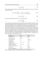
cathode–substrate distance d = 0.05 m, the number of elastic collisions of electrons with gas
atoms is small and the energy loss is insignificant.


2
q
1
q
2
3
1
x
b
0

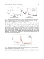
Fig. 12. Irradiation of the sample by the gas-discharge plasma flux: (1) insulating substrate,
(2) directed flux of the low-temperature plasma, and (3) temperature sensor at the lower
surface
It is known that whether series (34) converges or not depends on the value of at/b
2
: the
greater this parameter, the better the convergence. To find an exact solution at small at/b
2

(for example, at the initial stage of the process), it is necessary to leave 11–12 terms of the
series (Malkovich, 2002). In this study, we took into account 12 terms of sum (34).
As was noted earlier, the boundary-value problem is rather difficult to solve analytically,

because (41) contains the ratio of series K
1
and K
2
. Therefore, the proposed algorithm was
implemented by applying the Maple 8 program package. Using (41), we constructed the
dependences of temperature gradient ΔT in the substrate on the process time (Fig. 14).
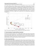
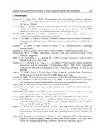
As is seen from Fig. 14a, the curves first sharply ascend. This is because the substrate, being
thin, heats up rapidly. In other words, incident flux q
1
(ε) passes through the sample almost
instantly without noticeable energy losses and goes away from the lower surface, rapidly
causing a temperature difference. When the irradiation time is long, the sample heats up at a
constant temperature gradient (Fig. 14a).
It is this circumstance that may be responsible for the so-called “thermal shock” (Kartashov,
2001), when thin samples are almost instantly destroyed once the discharge power exceeds a
critical value. Indeed, arising thermal stresses are determined by the temperature gradient,
which rapidly runs through intermediate values and reaches a maximum virtually at the
very beginning of the process (Fig. 14a). The simulation data suggest that the transient time
increases as the thermal diffusivity of the sample decreases or it gets thicker, thermal action
q
1
(ε) being the same. It is evident that this statement completely agrees with the theory of
heat transfer: a more massive sample reaches the stationary state for a longer time. In
addition, a material with a lower thermal conductivity will have a higher temperature
gradient, which will be established for a longer time. The rigorous solution of this problem
implies a combined consideration of the equations of heat transfer and thermoelasticity
(Samarskii & Vabishchevich, 1996).

Heat Transfer – Engineering Applications

110
0
600
T
, K
400 1000800600200
t
,
s
500
400
300
1
2
3
4

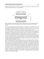
Fig. 13. Lower surface temperature vs. time: I = (1) 50, (2) 80, (3) 120, and (4) 140 mA. The
voltage applied to the electrodes is 2 kV, the pressure is 1.5 Torr, and the working gas is air

100
80
60
40
20
00
,
40
,

8
t
,

s
4
3
2
1
100
80
60
40
20
0 400 800
t
,

s

T
,
K
4
3
2
1

(a) (b)
Fig. 14. Temperature difference between the upper and lower surfaces for an irradiation

time of (a) 1 and (b) 1200 s. I = (1) 50, (2) 80, (3) 120, and (4) 140 mA
At high t, the temperature difference takes on a constant value (Fig. 14b). Therefore, failure
of the sample at the final stage is unlikely. The model proposed was also experimentally
verified using KÉF-32 silicon samples measuring 1×1×0.1 cm. The temperature of the sample
was controlled by varying the plasma flux irradiation parameters: voltage from 2.6 to 5.2 kV
and current from 24 to 80 mA. The irradiation duration was 10 min. The thermophysical
parameters of the material were matched to the process conditions. The temperatures of the
upper (exposed) and lower surface were measured by a Promin’ micropyrometer. The
surface temperatures and temperature gradient are listed in the table.
Temperature Measurement of a Surface Exposed to a
Plasma Flux Generated Outside the Electrode Gap

111
The disagreement between the calculated and experimental values of the temperature
difference does not exceed 12%, which confirms the adequacy of the estimation method.
The proposed method was applied for temperature measurement of a surface exposed to an
off-electrode plasma flux during research of etch-rate-temperature characteristic. In the
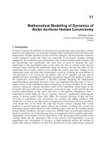
plasma etching mode of treatment the etch-rate–temperature characteristic is as shown in
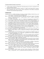
Fig. 15a. Notice that for every discharge current the etch rate is maximal at 360 K, the
vaporization temperature of SiF
4
. This point corresponds to the best conditions for etch-
product removal. As the wafer temperature is raised further, the etch rate falls due to
decrease in the amount of process gas adsorbed by SiO
2
, in accord with earlier results
(Ivanovskii, 1986; Kireyev & Danilin, 1983; Kireev et al., 1986).
In the reactive ion etching mode the temperature dependence is not so simple, as can be
seen from Fig. 15b. At a discharge current as weak as 50 mA (Fig. 15b, curve 1), the etch rate
is almost unaffected by wafer-temperature variation, because the etch rate in this case is

determined by the density of F
–
ions, as noted above. At 325–360 K, etching is possible
because the SiO
2
surface is almost free from particles that could impede etch-product
removal.
At stronger discharge currents, quite distinct behavior is observed (Fig. 15b, curves 2–4). The
reason is that the removal of SiF
4
is impeded by the species (F
–
ions, reactive species, and
reaction products) that have accumulated on and underneath the SiO
2
surface, with the
result that etching occurs only at wafer temperatures above 360 K, the vaporization
temperature of SiF
4
. As the wafer temperature increases from 360 K, the etch rate rises to a
maximum. Notice that the temperature of maximum etch rate depends on the discharge
current, being 390, 422, and 440 K for 80, 120, and 140 mA, respectively. An increase in wafer
temperature weakens interatomic bonding in the SiO
2
, making the material more susceptible
to sputtering. Further, the higher the discharge current, the more ions penetrate the SiO
2
to
enter into reactions there. As a result, the product species should migrate more slowly
toward the surface with increasing discharge current at a fixed wafer temperature. Higher

temperatures are therefore required to remove the products. The sharp fall in etch rate is
attributable to increase in ion penetration depth; this factor seriously hinders removal of
etch products (SiF
4
) with growing wafer temperature. Plasma processing in this case is
basically fluorine-ion doping of a SiO
2
surface layer and sputter etching. High temperature
breakdown of the photoresist was found to occur at 440 K, showing up as a faster fall in etch
rate with wafer temperature (etch rate should be the same in unmasked and opened areas).
Breakdown starts from the edges of the mask and causes etch taper (Fig. 16a), which will
guide ions just into trenches and so determine the trench profile (Fig. 16b). As the etch taper
grows, so do its angles and the etch profile becomes a sinusoid (V.A. Kolpakov, 2002). This
property is useful for making diffractive optical elements with a sinusoidal micropattern
(Soifer, 2002).
6. Results and discussion: Quality of surface treatment
Figure 17 displays trench profiles obtained by off-electrode plasma etching at discharge
currents of 50, 80, and 120 mA and oxygen percentages corresponding to maximum etch
rates. Prior to photoresist stripping, processed wafers were examined and found to be free
from etch undercut, an indicator of etching anisotropy. It can be seen from Fig. 17 that the
profile approaches a vertical-walled pattern with growing discharge current, as predicted
earlier. For example, a plasma with a current of 50 mA and a pressure of about 11 Pa is

Heat Transfer – Engineering Applications

112
deficient in F
–
ions, but these rarely collide with process-gas molecules and so have energies
as high as 100–500 eV (see Eq. (11)). Favorable conditions thus arise for the reflection of F

–

ions from trench sidewalls toward the center of the bottom. In this case the sidewalls may
deviate from the normal by an angle as large as 70°–75° (Fig. 17a). At a higher density of F
–

ions (current 80 mA, pressure 20 Pa), the ions strike the SiO
2
surface with a lower energy
and so are more likely to enter surface reactions, mostly at the site of landing. Further, when
isolated from other factors, the increase in reactive-species density is known to reduce the
sidewall deviation to 10°–20° (Moreau, 1988b).

120
100
80
40
60
20
0
350 450 550
Т
,
К
V
pht
, nm min.
/
4
3

2
1
280
300
240
200
160
120
80
0
40
V
iht
, nm min./
350 400 450
Т
, К

(a) (b)
Fig. 15. Etch rate vs. wafer temperature for (a) plasma etching or (b) reactive ion etching in a
CF
4
–O
2
plasma at discharge currents of (1) 50, (2) 80, (3) 120, and (4) 140 mA
Figure 17b,c shows that the trench bottoms meet the requirements of microelectronics
manufacturing: they are smooth and free from acute angles. Moreover, etching at 120–140 mA
and 25–33 Pa was found to produce trenches with vertical walls and a smooth bottom (Fig.
17d, e, f). Finally, the pressures employed satisfy the conditions given in (Orlikovskiy, 1999a).
Thus, all the trench profiles presented could find use in microelectronics (Moreau, 1988b;

Muller & Kamins, 1986) and diffractive optics (Soifer, 2002).
Off-electrode plasma etching in a CF
4
–O
2
plasma was also applied to other materials used in
microelectronics, as well as in diffractive optics. The respective etch rates are listed in the
table. At the same time, it was observed that fairly thick deposit is formed on the cathode
during etching (Fig. 18). Figure 19 is an x-ray diffraction pattern (Mirkin, 1961) from the
deposit; it indicates elements and compounds present in the process gas (C), the etched
material (SiO
2
, SiC, Si, As
2
S
3
, and C), and the etch mask (Cr
2
O
3
, CrO
3
, C, and H
2
). Cathode
deposit also includes large amounts of compounds containing the cathode material and
different oxides. On the other hand, it is free from fluorine, a fact suggesting that fluorine is
totally involved in etching (as part of reactive species). Moreover, the presence of the etched
material in the deposit implies that the plasma ensures etch-product removal. It follows that
the working plasma species (F

–
ions) move toward the wafer, whereas the product ones
Temperature Measurement of a Surface Exposed to a
Plasma Flux Generated Outside the Electrode Gap

113
toward the cathode. This result supports the mechanisms presented above. It is in accord
with earlier research (V.A. Kolpakov, 2002).


(a) (b)
Fig. 16. (a) Etch taper due to high-temperature photoresist breakdown and (b) the
corresponding trench profile. Etching is carried out at a discharge current of 140 mA, a
cathode voltage of 2 kV, and a wafer temperature of 440 K


(a) (b) (c)

(d) (e) (f)
Fig. 17. Images of trenches obtained by etching in CF
4
–O
2
plasma at different discharge
currents, optimal oxygen percentages, and a cathode voltage of 2 kV. The discharge currents
are (a) 50, (b, c) 80, and (d, e, f) 120 mA. The oxygen percentages are (a) 0.5, (b, c) 0.8, and (d,
e, f) 1.3%
Thus, even with highly contaminated process gas and wafer surface, off-electrode plasma
etching does not involve interactions other than a useful one (between reactive species and
wafer-surface molecules), allowing one to take less expensive gases.

Heat Transfer – Engineering Applications

114
Etching uniformity is among major concerns in microfabrication, because etch rate can vary
in a complicated manner over the wafer surface (Ivanovskii, 1986; Kovalevsky et al., 2002;
Poulsen & Brochu, 1973). In essence, all the recent improvements in plasma etching
technology aim to give high etching uniformity and rate; hence the high complexity and cost
of the equipment.


Fig. 18. Cathode surface after etching (magnification ×36)



Fig. 19. X-ray diffraction pattern (wavelength 0.154 nm) from cathode deposit, with
t denoting the x-ray reflection angle from the atomic planes
Our evaluation of off-electrode plasma etching in terms of uniformity, for a wafer of
diameter 100 mm, showed that both the plasma etching and the reactive ion etching mode
are uniform within 1% over the whole wafer. Etch profile was measured in different areas
on the wafer, and etch depth was found to be almost the same. The minor variations in etch
depth are in all likelihood linked with surface imperfections (lattice defects, contamination,
etc.) rather than the plasma conditions.
Temperature Measurement of a Surface Exposed to a
Plasma Flux Generated Outside the Electrode Gap

115
7. Conclusion
It has been shown that a major feature that distinguishes the high-voltage gas discharge
from the existing discharges is that the former can be induced in the dark Aston space,

provided an anode hole. This feature allows to generate a low-temperature plasma flux
outside the electrode gap.
Based on our experiments, a method for estimating the surface temperature of a sample
irradiated by a low-temperature plasma flux is produced. The relationships obtained in this
paper make it possible to evaluate the surface temperature directly at the site exposed to the
plasma flux. A slight excess of the theoretical estimate seems to be associated with the fact
that the plasma flux is incompletely absorbed by the solid: part of the flux is reflected from
the surface, decreasing the gradient. During ion–plasma processing, the temperature
gradient in the sample may become very high according to the geometry and material of the
sample, as well as to the amount of the thermal action.
The method makes it possible to trace the surface temperature of a sample being etched by
directed low-temperature plasma fluxes in a vacuum. This opens the way of improving the
quality of micro- and nanostructures by stabilizing the process temperature and optimizing
the rate of etching in the low-temperature plasma.
The phenomenon of thermal shock taking place at ion–plasma processing of flat surfaces is
theoretically explained. It is shown that the failure probability of thin samples is the highest
early in irradiation under the action of rapidly increasing thermal stresses. To determine the
critical power of the discharge, it is necessary to jointly solve the equations of heat
conduction and thermoelasticity.
Among disadvantages of the method is the neglect of the temperature dependence of
thermophysical parameters. This point becomes critical for semiconductors operating in a
wide temperature range. As a result, the temperature gradient versus process time
dependence becomes ambiguous. A more rigorous solution can be obtained by applying
numerical methods to the direct problem of heat conduction with mixed boundary
conditions. This would be a logical extension of this investigation.

8. Acknowledgment
The work was financially supported by the RF Presidential grant # NSH-7414.2010.9, the
Program of the President of the Russian Federation for Supporting Young Russian Scientists
(grant no. MD-1041.2011.2) and the Carl Zeiss grant # SPBGU 7/11 KTS.

9. References
Orlikovskiy, A.A. (1999a). Plasma Processes in Micro- and Nanoelectronics, Part 1: Reactive
Ion Etching. Mikroelektronika, Vol. 28, No. 5, pp. 344–362 (In Russian)
Alifanov, O. M. (1983). Inzhen.Fizich. Zhurnal. Vol. 45, No. 5, p.p. 742-752 (In Russian)
Alifanov, O. M. (1994). Inverse Heat Transfer Problem, Springer, New York
Bartenev, G. M. & Barteneva, A. G. (1992). Relaxation Properties of Polymers, Khimiya,
Moscow (In Russian)
Bechstedt, F. & Enderlein, R. (1988). Semiconductor Surfaces and Interfaces, Akademie-Verlag,
Berlin
Carslaw, H. S. & Jaeger, J. C. (1956). Conduction of Heat in Solids, Clarendon Press, Oxford

Heat Transfer – Engineering Applications

116
Chernetsky, A. V. (1969). Introduction into Plasma Physics, Atomizdat Publishers, Moscow (In
Russian)
Chernyaev, V.N. (1987). Fiziko-khimicheskie protsessy v tekhnologii REA (Physical and Chemical
Processes in Electronics Manufacture), Vysshaya Shkola, Moscow (In Russian)
Ditkin, V. A. & Prudnikov, A. P. (1966). Integral Transforms and Operational Calculus,
Pergamon, Oxford
Doh Hyun-Ho et al. (1997). Effects of bias frequency on reactive ion etching lag in an
electron cyclotron resonance plasma etching system. J.Vac. Sci. and Technol. A., Pt 1,
Vol.15, No. 3, p.p. 664-667
Flamm, D.L. (1979). Measurements and Mechanisms of Etchant Production During the
Plasma Oxidation of CF
4
and C
2
F
6

. Solid State Technol., Vol. 22, No. 4, pp. 109–116
Gerlach-Meyer, V. (1981). Ion Enhanced Gas-Surface Reactions: A Kinetic Model for the
Etching Mechanism. Surface Sci., Vol. 103, No. 213, pp. 524–534
Harsberger, W.R. & Porter, R.A. (1979). Spectroscopic Analysis of RF Plasmas. Solid State
Technol., Vol. 22, No. 4, pp. 90–103
Hebner, G.A. et al. (1999). Influence of surface material on the boron chloride density in
inductively coupled discharges. J.Vac. Sci. and Technol. A., Vol.17, No. 6, p.p. 3218-
3224
Horiike, Y. (1983). Dry Etching: An Overview. Jap. Annual Revue in Electronics, Computers and
Telecommunicated Semiconductor Technologies, Vol. 8, pp. 55–72
Ivanovskii, G.F. (1986). Ionno-plazmennaya obrabotka materialov (Plasma and Ion Surface
Engineering), Radio i Svyaz’, Moscow (In Russian)
Izmailov, S. V. (1939). On the thermal theory of electron emission under the impact of fast
ions. Russian Journal of Experimental and Theoretical Physics, Vol.9, No. 12, p.p. 1473 –
1483 (In Russian)
Kartashov, E. M. (2001). Analytical Methods in the Theory of Heat Conduction in Solids,
Vysshaya Shkola, Moscow (In Russian)
Kazanskiy, N.L. & Kolpakov, V.A. (2003). Studies into mechanisms of generating a low-
temperature plasma in high-voltage gas discharge. Computer Optics, No. 25, p.p.
112-117 (In Russian)
Kazanskiy, N. L. et al. (2004). Anisotropic Etching of SiO
2
in High-Voltage Gas-Discharge
Plasmas. Russian Microelectronics, Vol. 33, No. 3, p.p. 169-182
Kikoin, I. K. (Ed.). (1976). Tables of Physical Quantities, Atomizdat, Moscow (In Russian)
Kireyev, V. Yu. & Danilin, B. S. (1983). Plasmo-chemical and ion-chemical etching of
microstructures, Radio i Svyaz (Radio and Communications) Publishers, Moscow (In
Russian)
Kireev, V.Yu. et al., (1986). Ion-Enhanced Dry Etching. Elektron. Obrab. Mater. (Electron
Treatment of Materials), No. 67, pp. 40–43 (In Russian)

Kolpakov, A.I. & Kolpakov, V.A. (1999). Dragging of Silicon Atoms by Vacancies Created in
Molten Aluminum under Ion–Electron Irradiation. Technical Physics Letters, Vol. 25,
No. 15, p. 618
Kolpakov, V.A. (2002). Modeling the High-Voltage Gas-Discharge Plasma Etching of SiO
2
.
Mikroelektronika, Vol. 31, No. 6, pp. 431–440 (In Russian)
Kolpakov, A. I. et al. (1996). Ion-plasma cleaning of low-power relay contacts. Electronics
Industry, No. 5, p.p. 41-44 (In Russian)
Temperature Measurement of a Surface Exposed to a
Plasma Flux Generated Outside the Electrode Gap

117
Kolpakov, A. I. & Rastegayev, V. P. (1979). Calculating the electric field of a high-voltage gas
discharge gun, VINITI, Moscow (In Russian)
Kolpakov, V. A. (2004). Candidate’s Dissertation, SGAU & ISOI RAN, Samara (In Russian)
Kolpakov, V. A. (2006). Studying an Adhesion Mechanism in Metal – Dielectric Structures
Following the Surface Ion-Electron Bombardment. Part 1. Modeling an Adhesion
Enhancement Mechanism. Phys. and Chem. of Mat. Proc., No. 5, pp. 41-48 (In
Russian)
Komine Kenji et al. (1996). Residuals caused by the CF
4
gas plasma etching process. Jap. J.
Appl. Phys. Pt.1, Vol. 35, No. 5b, p.p. 3010-3014
Komov, A.N. et al. (1984). Electron-Beam Soldering Machine for Semiconductor Devices.
Prib. Tekh. Eksp. (Scientific Instruments and Methods), No. 5, pp. 218–220 (In Russian)
Kovalevsky, A. A. et al. (2002). Studies into the process of isotropic plasmo-chemical etching
of silicon dioxide films. Mikroelektronika, Vol. 31, No. 5, p.p. 344-349 (In Russian)
Malkovich, R. Sh. (2002). Technical Physics Letters, Vol. 28, No. 21, p. 923
Matare, G. (1974). Electronics of semiconductor defects, Mir Publishers, Moscow (In Russian)

McLane, G.F. et al. (1997). Dry etching of germanium in magnetron enhanced SF
6
plasmas.
J.Vac. Sci. and Technol. B., Vol. 15, No. 4, p.p. 990-992
Mirkin, L.I. (1961). Spravochnik po rentgenostrukturnomu analizu polikristallov (Handbook of X-
ray Crystallography for Polycrystalline Materials), Gosudarstvennoe Izdatel’stvo
Fiziko-Matematicheskoi Literatury Publisher, Moscow (In Russian)
Miyata Koji et al. (1996). CF
x
radical generation by plasma interaction with fluorocarbon
films on the reactor wall. J.Vac. Sci. and Technol. A., Vol. 14, No. 4, p.p. 2083-2087
Molokovsky, S. I. & Sushkov, A. D. (1991). High-intensity Electron and Ion Beams,
Energoatomizdat Publishers, Moscow (In Russian)
Moreau, W. M. (1988a). Semiconductor Lithography: Principles, Practices and Materials. Chap. 1,
Plenum, New York
Moreau, W.M. (1988b). Semiconductor Lithography: Principles, Practices, and Materials. Chap. 2,
Plenum, New York
Muller, R.S. & Kamins, T.I. (1986). Device Electronics for Integrated Circuits, Wiley, New York
Orlikovskiy, A.A. (1999b). Plasma Processes in Micro- and Nanoelectronics, Part 2: New-
Generation Plasmochemical Reactors in Microelectronics. Mikroelektronika, Vol. 28,
No. 6, pp. 415–426 (In Russian)
Popov, V. K. (1967). Fiz. Khim. Obrab. Mater. (Physics and Chemistry of Materials Processing),
No. 4, p.p. 11-24 (In Russian)
Poulsen, R.G. & Brochu, M. (1973). Importance of Temperature and Temperature Control in
Plasma Etching, Si Bricond Silicon, New-Jersey
Raizer, Yu.P. (1987). Fizika gazovogo razryada (Gas-Discharge Physics), Nauka, Moscow (In
Russian)
Rykalin, N. N. et al. (1978). Principles of Electron-beam Material Processing, Mashinostroyenie
(Mechanical Engineering) Publishers, Moscow (In Russian)
Samarskii, A. A. & Vabishchevich, P. N. (1996). Computational Heat Transfer, Wiley,

Chichester
Sarychev, M. E. (1992). Non-liner Diffusion Model of Polymer Resist Plasma-chemical
Etching Process. Simulation of Technological Processes of Microelectronics. Tr.
FTIAN (FTIAN Annals), Vol. 3, p.p. 74-84 (In Russian)

Heat Transfer – Engineering Applications

118
Soifer, V.A. (Ed.). (2002). Methods for Computer Design of Diffractive Optical Elements, Wiley,
New York
Tikhonov, A. N. & Samarskii, A. A. (1964). Equations of Mathematical Physics, Pergamon,
Oxford
Tikhonov, A. N. & Arsenin, V. Ya. (1977). Solutions of Ill-Posed Problems, Halsted, New York
Vabishchevich, P. N. & Pulatov, P. A. (1986). Inzhen.Fizich. Zhurnal. Vol. 51, No. 3, p.p. 470-
474 (In Russian)
Vagner, I.V. et al. (1974). Simple Beam-Forming Arrangement for Generating Arbitrarily
Shaped Electron Beams under High-Voltage Gas Discharge. Zh. Tekh. Fiz.(Russian
Journal of Technical Physics), Vol. 44, No. 8, pp. 1669–1674 (In Russian)
Valiev, K. A. et al. (1985). Polymer Plasma-chemical Etching Mechanism. Dokl. Akad. Nauk
SSSR (Sov. Phys. Dokl), Vol. 30, p. 609 (In Russian)
Valiev, K. A. et al. (1987). Investigation of Etching Kinetics of Polymetilmetacrelat in Low-
temperature Plasma. Poverkhnost’ (Surface), No. 1, p.p. 53-57 (In Russian)
Woodworth, J.R. et al. (1997). Effect of bumps on the wafer on ion distribution functions in
high-density argon and argon-chlorine discharges. Appl. Phys. Lett., Vol. 70, No. 15,
p.p. 1947-1949
Part 2
Heat Conduction – Engineering Applications

6
Experimental and Numerical Evaluation

of Thermal Performance of Steered
Fibre Composite Laminates
Z. Gürdal
1
, G. Abdelal
2
and K.C. Wu
3

1
Delft University of Technology
2
Virtual Engineering Centre, University of Liverpool
3
Structural Mechanics and Concepts, NASA Langley Research Center
1
The Netherlands
2
UK
3
USA
1. Introduction
For Variable Stiffness (VS) composites with steered curvilinear tow paths, the fiber
orientation angle varies continuously throughout the laminate, and is not required to be
straight, parallel and uniform within each ply as in conventional composite laminates.
Hence, the thermal properties (conduction), as well as the structural stiffness and strength,
vary as functions of location in the laminate, and the associated composite structure is often
called a “variable stiffness” composite structure. The steered fibers lead not only to the
alteration of mechanical load paths, but also to the alteration of thermal paths that may
result in favorable temperature distributions within the laminate and improve the laminate

performance. Evaluation of VS laminate performance under thermal loading is the focus of
this chapter. Thermal performance evaluations require experimental and numerical analysis
of VS laminates under different processing and loading conditions. One of the advantages of
using composite materials in many applications is the tailoring capability of the laminate,
not only during the design phase but also for manufacturing. Heat transfer through variable
conduction and chemical reaction (degree of cure) occurring during manufacturing (curing)
plays an important role in the final thermal and mechanical performance, and shape of
composite structures.
Three case studies are presented in this chapter to evaluate the thermal performance of VS
laminates prior to and after manufacturing. The first case study is a numerical analysis that
investigates the effect of variable conductivity within the VS laminate on the temperature
and degree of cure distribution during its cure cycle. The second case study is a numerical
analysis that investigates the transient thermal performance of a rectangular VS composite
laminate. Variable thermal conductivity will affect the temperature profile and results are
compared to a unidirectional composite. The effect of fiber steering on transient time and
steady state solutions is compared to the effect of unidirectional fibers. The third case study
is an experimental one that was conducted to evaluate the thermal performance of two
variable stiffness panels fabricated using an Advanced Fiber Placement (AFP) Machine.

Heat Transfer – Engineering Applications

122
These variable stiffness panels have the same layup, but one panel has overlapping bands of
unidirectional tows (which lead to thickness variations) and the other panel does not.
Results of thermal tests of the variable stiffness panels are presented and compared to
results for a baseline cross-ply panel. These case studies will show the impact of the steering
parameters of variable stiffness laminates during the manufacturing and design phases.
2. Preliminaries
Laminated composite plates structures, which have high strength-to-weight and stiffness-to-
weight ratios, are extensively used in aerospace and automotive applications that are

exposed to elevated temperatures. Accurate knowledge of the thermal response of these
materials is essential for the optimum design of thermal protection systems. In some
circumstances, high thermally induced compressive stresses may be developed in the
constrained plates and can therefore lead to buckling failures. In addition, conductivity of
the fiber-reinforced layers is direction dependent, and therefore the degree of anisotropy of
the laminate can substantially influence the conductivity of the laminate in different
directions.
Variable stiffness laminates with steered fiber paths offer stiffness tailoring possibilities that
can lead to alteration of load paths, resulting in favorable temperature distributions within
the laminate and improved laminate structural performance. A further generalization of this
idea was to allow the direction of the fiber orientation angle variation to be rotated with
respect to the coordinate direction x, rather than limiting it to be only along the x-axis or the
y-axis. As shown in Figure 1, a fiber orientation angle T
0
is defined at an arbitrary reference
point A with respect to direction x that is rotated by an angle ϕ from the coordinate axis x.
The fiber orientation angle is then assumed to reach a value T
1
at point B located a
characteristic distance d from point A. With the linear variation of the fiber orientation angle
between the points A and B, the equation for the fiber orientation angle along this reference
path takes the form,




  
10 0
() ( )
x

xTTT
d

(1)

A variable stiffness layer can be represented with three angles and a characteristic distance
to represent a single layer. Assuming the characteristic distance to be associated with a
geometric property of the part, representation of a single curvilinear layer may be specified
by ϕ<T
0
|T
1
>. A conventional representation, a  sign in front of either ϕ or <T
0
|T
1
> means
that there are two adjacent layers with equal and opposite variation of the fiber orientation
angle. A laminate with  ϕ <T
0
|T
1
> designation will have four curvilinear layers: a  ϕ
<T
0
|T
1
> pair along the +ϕ direction, and a  ϕ <T
0
|T

1
> pair along the -ϕ direction.
Variable stiffness (VS) laminates were introduced by (Gürdal and Olmedo, 1993; Olmedo
and Gürdal, 1993). Examples of fiber orientation angle tailoring include theoretical and
numerical studies by (Banichuk, 1981; Banichuk and Sarin, 1995), (Pedersen, 1991, 1993)],
and (Duvaut et al., 2000). In a design study by (Gürdal et al., 2008), analyses of variable
stiffness panels for in-plane and buckling responses are developed and demonstrated for
two distinct cases of stiffness variation. Later optimization studies (Setoodeh et al., 2006,
2007, 2009) were carried out demonstrating the theoretical benefits of variables stiffness
laminates in improving structural performance. For variable stiffness laminates, which also
Experimental and Numerical Evaluation of
Thermal Performance of Steered Fibre Composite Laminates

123
have spatially variable coefficients of thermal expansion along with the stiffness properties,
spatial variation of residual stresses are induced. More recent studies investigated the effect
of thermal residual stresses on the mechanical buckling performance of variable stiffness
laminates (Abdalla et al., 2009).


Fig. 1. Reference path definition of a variable layer
The degree of damage and strength degradation of the VS laminates subjected to severe
thermal environments is a major limiting factor in relation to service requirements and
lifetime performance. In order to predict these thermally induced stresses, a detailed
understanding of the transient temperature distributions is essential. A number of studies
of isotropic materials and composites have been carried out to explore the potentially
complicated time dependence of the temperature field (Hetnarski, 1996). There have also
been numerous analytical models developed over the years to describe the transient
behaviors of commonly encountered geometries (Mittler et al., 2003; Obata and Noda,
1993).

Alternatively, in order to endure the severe thermal loads, many structural components are
made such that they are non-homogeneous. Thermal barrier coatings of super alloys on
ceramics used in jet engines, stainless steel cladding of nuclear pressure vessels, and a great
variety of diffusion-bonded materials used in microelectronics may be mentioned as some
examples. Typically, these non-homogeneous materials and structures are subjected to
severe residual stresses upon cooling from their processing temperatures. They may also
undergo thermal cycling during operations. Depending on the temperature gradients, the
underlying thermal stress problem may be treated as a thermal shock problem or as a quasi-
static isothermal problem in the sense that the problem may still be time-dependent but
with no variation of temperature within the composite solid.
Clearly, there is an actual need for investigating the thermal transients developed within VS
composites. However, because of the inherent mathematical difficulties, thermal analyses of
non-homogeneous structural materials are considerably more complex than in the
corresponding homogeneous case. Numerical techniques such as the finite element method
x

A

B
y

d
T
0
T
1

x
'
y

'

Heat Transfer – Engineering Applications

124
are of great importance for solving for temperature profile and stress distribution in VS
laminates.
3. Numerical heat conduction analysis
The main purpose of this section is to study a finite-element approximation to the
solution of the transient and steady-state heat conduction with different boundary
conditions in a two-dimensional rectangular region. A Galerkin finite element formulation is
applied to the 2-D heat conduction equation using four planar finite elements. The
composite conduction and capacitance matrices are derived as functions of the steered fiber
orientation angles.
3.1 Two-dimensional heat conduction in Cartesian coordinates
The governing differential equation for a two dimensional heat conduction problem is given
by,

x,xx y,yy p,t
k
T
k
T
Q
c
T





(2)

where T is the temperature, k
x
and k
y
are material conductivity along the x- and y-
directions, ρ is material density, Q is the inner heat-generation rate per unit volume, and c
p

is material heat capacity.
Boundary conditions are described as,

0
1
,,
2
,,
3
(specified temperature)
(specified heat flow)
()(convection boundar
y
condition)
SS
xx yy
SS
xx yy s e
SS

TT
kT kT q
kT kT hT T






(3)
where h is the convection coefficient, Ts is an unknown surface temperature, Te is a
convective exchange temperature, and q is the incident heat flow per unit surface area.
3.2 Heat conduction simulation using finite element
Using a typical Galerkin finite element approach to Eqn. (2) the residual equation for a plate
with unit thickness assumes the form,



x,xx y,yy p,t
NkT kT Q cTdxdy0

 




(4)

where the temperature field function is expressed in terms of the interpolation functions as,








e
TNT

(5)

Integration of Eqn. (4) by parts yields,





T
T
e
,x x ,x ,y y ,y
TT
p,ti
V
N k N N k N dx dy T
c N N dx dy T Q N dV N q dS

 
 

 
 




  

(6)

Experimental and Numerical Evaluation of
Thermal Performance of Steered Fibre Composite Laminates

125
where q is the heat flow through unit area. Finally the governing equation takes the form,








Th T Q h
KK T CT F R R 

(7)
where,











3
T
composite conduction matrix, /
composite convection matrix, /
unknown nodal temperature vector, .
C capacitance matrix, J/
composite element
T
C
V
T
h
S
T
p
V
e
T
K Watt C N k N dV
KWattChNNdS
TC
CcNNdV

TTt
F





 














3
2
3
nodal force vector, Watt =
internal-heat vector, /
convection heat vector, /
interpolation function,
T

s
V
T
Q
V
T
h e
S
e
NqdS
RWattmCQNdV
RWattmChTNdS
NTNT









Introducing the normalized lamination parameters [Gürdal et al., 1999],














1/2
1234
1/2
1/2
2
1234
1/2
, , , cos2 , sin2 ,cos 4 ,sin 4
, , , 12 cos2 , sin2 ,cos4 ,sin 4
VVVV dz
WWWW z dz

(8)

the conductivity matrix [k] can be expressed as a function of the lamination parameters,



 
01122
kKKVKV

(9)



















11 22 11 22
01
11 22 11 22
22 11
2
22 11
0.5 0 0.5 0
00.5 00.5
00.5
0.5 0
kk kk

KK
kk kk
kk
K
kk

(10)

where k
11
and k
22
are the conductivity of the lamina along and perpendicular to the fibers
directions respectively.
The finite element solution of time-dependent field problems produces a system of linear
first-order differential equations in the time domain. These equations must be solved before
the variation of the temperature T in space and time is known. There are several procedures
for numerically solving Eqn. (7). Finite difference approximation (central difference) in the
time domain is applied to generate a numerical solution,

 

 
  


 









TT TT TT
i1 i i i1
ttt
CKTCKT FF
222

(11)


Heat Transfer – Engineering Applications

126
If Δt (time increment) and the material properties are independent of time, Eqn. (11) can be
formulated as,














*
i1 i
AT PT F

(12)

where [A] and [P] are combinations of [C] and [K], and

 

*
1
2
TT
ii
t
FFF



.
3.3 Numerical stability techniques
Transient heat conduction problems can be solved by first discretizing the spatial
dimensions using the finite element method, then transforming the space-time partial
differential equation (PDE) into an ordinary differential equation (ODE) in time. The time
integration of the discrete Eqn. (7) is then performed using ODE integrators. These
integrators replace the time derivative by a finite difference approximation (forward,
central, or backward differences). This integration method is inexpensive per step, but

numerical stability requires using small time-steps. The numerical oscillations in the values
of {T} from one time-step to the next are related to




1
AP
, and can be avoided by applying
the following criteria (Segerlind, 1984),

 


det 0
2
ee
TT
CK
t





(13)
(Trujillo, 1977) has proposed an explicit algorithm that has a time-step fifteen times greater
than the conventional method used. (Hughes et al., 1982) proposed an element-by-element
implicit algorithm to solve Eqn. (7). (Zienkiwicz et al., 1980) proposed a procedure based on
systemic partitioning of the discrete Eqn. (7) and involving extrapolation.

4. Curing simulation of variable stiffness laminate
Thermoset polymers often release a significant heat of reaction during processing. The
chemical reaction that occurs during the curing of thermoset polymers plays an important
role in the process modeling of thermoset composites. The exothermic heat released during
the curing process can cause excessive temperatures in the interior of composites. Cure
kinetics that provide information on the curing rate and the amount of exothermic heat
release during the chemical reaction are important in the process simulation of composite
materials with thermoset polymers. Therefore, the inclusion of an accurate cure kinetics
model is essential for the processing simulation of thermoset composites. Several studies
have shown that amine-cured epoxy resins are governed by an autocatalytic reaction
(Johnston, 1997; Scott, 1991). The epoxy group that reacts with a primary amine produces a
secondary amine and then forms a tertiary amine. These reactions are also accelerated by the
catalytic action of the hydroxyl group that is formed as a by-product of the amine–epoxy
reaction.
The majority of heat transfer models for composites processing consider heat flow in the
through-thickness direction only (a one-dimensional model) or make the even simpler
assumption of a uniform laminate temperature (White and Hahn, 1992). More sophisticated
Experimental and Numerical Evaluation of
Thermal Performance of Steered Fibre Composite Laminates

127
models examining heat transfer in two and three dimensions have also been developed
(Bogetti and Gillespie, 1991). The resin chemical reaction is generally indicated by a time-
dependent measure known as the degree of cure, α, as in Equation (14) which is usually
defined based on a measure of the heat given off by bond formation as follows:

t
0
R
1dq

dt
Hdt






(14)

where (dq/dt) is the rate of heat generation and H
R
is the total amount of heat generated per
unit volume during a full reaction. The value of α can be easily determined using standard
differential scanning calorimetry (DSC) heat flow measurements. The heat generated due to
cure of the resin Q* is expressed as,

R
d
QH
dt




(15)

where dα/dt is designated as the cure rate and ρ is the composite material density.
A number of different models have been proposed to simulate the cure kinetics of various
resin systems. These models can be divided into two general types: mechanistic and

empirical. Mechanistic models use as their basis a detailed understanding of the chemical
reactions that take place throughout the cure process. Such models are not always practical
due to the complexity of the chemical reactions that can vary greatly from one resin system
to another depending on the combination of base resin, hardeners and catalysts.
Furthermore, most commercial resin systems are proprietary and the user is often
prohibited from even trying to determine their exact composition. Empirical models are
expressions derived to provide a fit to experimentally determined cure rates. Most cure
models employ Arrhenius-type equations, with the rate of reaction expressed as some
function of degree of cure and temperature. An example of a commonly used semi-
empirical expression for cured epoxy systems is (Scott, 1991):




12
1
exp /
n
m
ii i
d
YY
dt
YA ERT



 

(16)

where ∆E
i
are activation energies, R is the gas constant, and A
i
, m, n are experimentally-
determined constants. To account for the effect of glass transition on reaction rate, a
combination of expressions of the form of Eqns. (16) (Lee et al., 1982; White and Hahn, 1992)
and modified expressions of similar type have been used (Dusi et al., 1987; Cole et al., 1991).



12
1
n
m
d
YY
dt



 
(17)
where Y
i
are defined as in Eqn. (16) and m and n are other experimentally determined
constants. The parameter β is the ”isothermal degree of cure”, defined as the limiting degree
of cure at a given temperature. Its relation to the degree of cure is given by:

T

R
H(T)
H


(18)


Heat Transfer – Engineering Applications

128
where H
T
(T) is the total amount of heat that would be given off by isothermally curing the
resin at temperature T for infinite time.
4.1 Thermal-chemical model
A thermo-chemical model simulation requires the determination of the reaction kinetics of
each resin and thermal transport of the heat of reaction across the laminate panel to calculate
changes in the laminate temperature that affect thermal strains, and degree of cure that
affects resin modulus. The following mathematical equation is modeled applying transient
thermal analysis.


,1,2
p
i
j
Rv
ij
TTc

ckHQ
tx x t
ij


 



  


(19)
where ρ denotes the composite density, c
p
the specific heat, T the temperature, t the time, x
i

the spatial coordinates, and k
ij
the components of the thermal conductivity tensor. The
degree of cure c is defined as the ratio of the heat released by the reaction to the ultimate
heat of reaction H
R
, and Q
v
is the heat convection to the surrounding air in the autoclave.
Orthotropic conductivity is assumed for all materials so that values of k
11
, k

22
, and k
33
are
required. Assuming resin conductivity is isotropic and fibre conductivity is transversely
isotropic, a rule of mixture is used (Twardowski et al., 1993) to evaluate lamina thermal
conductivity:



11 11
2
22
2
22
.1.
1.
14
.12. . .tan
1. 1.
2. 1















  































ff f r
f
f
r
ff
r
KVK VK
V
B
V
KK a
B
VV
BB
K
B
Kf

(20)

where K
f11
, K
f22

are the longitudinal and transverse conductivities of the fibers, and K
r
is the
isotropic conductivity of the resin. These values are assumed as a function of temperature.
Laminate global conductivity is calculated as described in eqn. (9) and eqn. (10).
The lamina specific heat capacity is calculated using the following equation (Gürdal et al.,
1999),




1
1





fpff f prr
p
ff f prr
VC V C
C
VVC

(21)

where C
pf
and C

pr
are the respective specific heats of the fibers and resin, and are modelled
as a function of temperature. The internal heat generated due to the exothermic cure
reaction is described as in (White and Hahn, 1992),
Experimental and Numerical Evaluation of
Thermal Performance of Steered Fibre Composite Laminates

129


1
n
m
ERT
dc
Y
dt
YAe





(22)
where Y is the Arrhenius rate, R=8.31 J/Mol.K is the universal gas constant, A the frequency
factor, (m, and n) are experimentally-determined constants for a given material, and ΔE the
activation energy. The heat transfer coefficient for an autoclave of size (1.8 m x 1.5 m) is
measured and can be expressed as (Johnston, 1997),

52

20.1 9.3 (10 ) ( / )hPWmK


(23)
where P is the autoclave pressure.
4.2 Cure simulation using finite elements
A thermochemical model is used for calculation of temperature and the degree of cure in
composite components. Accurate prediction of these parameters is potentially useful to the
composites modeling in a number of ways. First of all, one of the main objectives of
processing thermoset composite materials is to achieve uniform cure of the matrix resin so
that a structure can attain its maximum stiffness, static and fatigue strength and resistance to
moisture and chemical degradation. Achieving maximum degree of cure in minimum time
would seem to indicate that a high temperature cure cycle be used. However, this approach
has other, potentially negative, implications for the cure process. For example, the rapid heat
evolution of the resin’s exothermic reaction at high temperatures can lead to a ‘runaway’
reaction as heat is generated more quickly than it can be removed, potentially resulting in
resin thermal degradation. It has also been found that the large spatial and temporal
gradients in resin degree of cure and temperature induced by rapid cure can be an
important source of process-induced stress (Levitsky and Shaffer, 1975; Bogetti, 1989),
especially in thick-section composites. Thermochemical model predictions are also
important to the simulation of other processing phenomena such as resin flow and the
generation of residual stress and deformation. One reason this is so is that temperature and
degree of cure are two of the most important ‘state’ variables used to predict composite
material properties during processing. Thus, prediction of everything from resin viscosity to
thermal expansion and resin cure shrinkage strains are dependent on thermochemical
model predictions.
The thermochemical model consists of a combination of analyses for heat transfer and resin
reaction kinetics. The model of (Bogetti and Gillespie, 1992) can be applied to general two-
dimensional composite modeling. It has the added capability of incorporating multiple
composite and non-composite materials as well as process tooling. Other important features

include the potential for improved boundary condition modeling using the autoclave
simulation and consideration of material property variation during processing. Also, by
integrating another model that considers resin flow, the effect of fiber volume fraction
variation during processing can also be considered.
The governing equation of the thermochemical model is the unsteady-state two-dimensional
anisotropic heat conduction equation with an internal heat generation term from the resin’s
exothermic curing reaction is modeled using Eqn. (19). The governing equations of the heat
transfer portion of the problem are solved employing the finite element approximation, and

Heat Transfer – Engineering Applications

130
time integration is performed as described in section 3.3 using a central finite difference
approximation.
The heat transfer equation, Eqn. (19), and the cure kinetics equations outlined in section 4.1
are coupled. Ideally, therefore, a coupled solution technique would be employed in which
both temperature and degree of cure would be solved in a single calculation. For the current
model, for each time increment, the temperature will be solved first at the discretized
locations (nodes) using the previous increment degree of cure (internal heat) and applied
boundary conditions. Then using the calculated temperature, the degree of cure and the
new internal heat generated are updated using Eqn. (22). Composite thermal properties that
are used in our simulation are listed in Table 1.

Specific heat capacity
(J/Kg.K)
C
pf
= 800

Thermal conductivity

(W/m.K)
k
fl
= 6.5
k
r
= 0.65
Fibre volume fraction V
f
= 0.6
Cure kinetic model H
R
= 590(10
3
),
ΔE = 66.9 KJ/gmole,
A =5.333E+5 /s,
m=0.79,
n=2.16,
α
0
=0.01
Table 1. Thermal material properties.
Boundary conditions considered on the two-dimensional simulation analysis are:

Convective heat transfer (applied on the top surface of the laminate) (q = h (T
e
-T), where h is
the heat transfer coefficient (see Eqn. (23)) and Te and T are the air and boundary
temperatures, respectively). Convective heat transfer is usually the dominant heat

transfer mechanism in an autoclave at temperatures normally encountered in thermoset
processing.

Adiabatic boundary (along the laminate's edges) (q = 0 or ∂T/∂n = 0, where n is the
surface normal vector).
4.3 Numerical results
The composite plate considered in this study is a mid-plane symmetric laminate with
dimensions (0.36m x 0.36m x 0.003m). It consists of 6 sub-laminates, each of which
consists of 4 layers [

ϕ

<T
0
|T
1
>], for a total of 24 plies. The laminate is made from
carbon/epoxy (AS4/3501) with material properties defined in Table 1. The analysis is
performed by discretizing the panel using a uniform mesh of rectangular four-noded
Kirchhoff plate elements. The transient response of the VS laminate and the different
shape of the heat transfer channels from the straight-fiber ones (to be discussed in the next
section), could affect both the temperature and degree of cure response. However,
performance of the simulation as a function of the autoclave time cycle showed that there
is no difference in thermal performance "in autoclave" between VS and straight fiber
composites.

Experimental and Numerical Evaluation of
Thermal Performance of Steered Fibre Composite Laminates

131

0 0.5 1 1.5 2 2.5 3
x 10
4
20
40
60
80
100
120
140
160
180
Autoclave time cycle, sec
Temperature, C

Fig. 2. Autoclave temperature cycle and temperature response of composite.

0 0.5 1 1.5 2 2.5 3
x 10
4
0
0.1
0.2
0.3
0.4
0.5
0.6
0.7
0.8
0.9

1
Autoclave time cycle, sec
Degree of cure

Fig. 3. Degree of cure of VS and straight-fiber composite.
The autoclave temperature cycle and the laminate thermal response at the composite plate
center are shown in Figure 2. The autoclave thermal cycle can be divided to three phases.
The first phase involves raising the autoclave air temperature from room temperature (25
ºC) to 107 ºC, and then holding this temperature for 1 hour. The second phase raises the
autoclave air temperature to 177 ºC and holds this temperature for 2 hours. The heat that is
Autoclave temperature c
y
cle
Laminate
thermal response

Heat Transfer – Engineering Applications

132
generated by the cure kinetics during the autoclave thermal cycle starts when the composite
panel temperature is close to 107 ºC. This internal heat leads to an increase in the composite
panel temperature, then the extra heat is transferred back to the autoclave air. Once the
epoxy is fully cured, there is no exothermic curing heat reaction. The degree of cure is
shown in Figure 3 as a function of the cure cycle time. The change in the degree of cure is
low during the initial phase of the autoclave thermal cycle, once the exothermic curing
reaction started, we can see faster curing until the autoclave air temperature is 177 ºC, then
curing slows down until it is fully cured. The main factor behind the similarity of curing of
VS and straight fibers is the composite panel is exchanging heat through the transverse
direction and not through the in-plane direction (as boundaries are isolated). Heat exchange
through boundaries will be affected by the in-plane fiber layout and is discussed in next

section.
5. Transient heat response of variable stiffness laminate
Clearly, there is an actual need for investigating the thermal transients developed within VS
composites. However, because of the inherent mathematical difficulties, thermal analysis of
non-homogeneous structural materials is considerably more complex than in the
corresponding homogeneous case. Numerical techniques such as finite element methods are
of great importance for solving for temperature profile and stress distribution.

This section investigates thermal transient analysis of rectangular variable stiffness
composite under uniform partial heat flux using finite element analysis. Variable thermal
conductivity will affect the temperature profile results compared to unidirectional
composite. The effect of the extra design parameter of variable stiffness laminates (steering
of fibers) on transient response is investigated. The need for cooling of a structural panel is
determined by transient time and boundary conditions. The transient solution of variable
stiffness laminate is compared to the unidirectional one. Later, the steady state temperature
profile is used to determine thermal stresses of the variable stiffness laminate compared to a
unidirectional one applying forced straight edge boundary conditions. The mechanics of
variable-stiffness laminates are discussed in (Abdalla et al., 2009).

5.1 Transient response
A two-dimensional finite element (FE) model describing heat transfer analysis of a variable-
stiffness composite laminate exposed to partial surface heating is illustrated in Figure 4. The
effect of fiber steering (T
0
, T
1
) on transient time and steady state solution is compared to
straight fibers. A Matlab computer program was written for the FE procedure discussed in
previous sections. The program has been used to evaluate the transient response of different
fiber steering. Material properties of the laminate are listed in Table 1. The composite wall is

assumed to have a uniform initial temperature; T
i
= 0 °C. The results presented here are for a
partially heated plate at input heat energy of h
Input
= 100 W/(m
2
). The accuracy of the results
was verified by comparing the straight-fiber results to the ABAQUS transient heat transfer
analysis. Boundary conditions for laminate edges act as a heat sink and are fixed at T = 0 °C.
The transient response of a heat conduction problem can be characterized by two
parameters. One parameter is the time to reach steady state. A longer time to reach steady
state is better for thermal protection panels as it allows more time for the structure to absorb
heat, which reduces thermal stresses and delays the ablation process that degrades material
properties. The second parameter is the maximum temperature reached at the center of the
Experimental and Numerical Evaluation of
Thermal Performance of Steered Fibre Composite Laminates

133
panel. A lower maximum temperature is desirable for the same reasons to reduce thermal
stresses, which improves buckling response and delays the ablation process. A variable
stiffness laminate adds more three design parameters (
ϕ, T
0
, T
1
) that can be used to achieve
the optimal thermal performance. For example, Figure 5 compares the performance of
variable stiffness panels while varying T
0

and T
1
versus the straight-fiber laminate
performance. The transient time is normalized by the maximum transient time that can be
achieved using a straight-fiber laminate, and the maximum temperature at plate center is
normalized by the minimum temperature achieved using a straight-fiber laminate. The
straight-fiber laminate is represented by the heavy line, and is a symmetric angle-ply layup
that has a linear variation of a pair of fiber angles [

]
s
, so the 0º and 90º laminates have the
same maximum temperature and transient time. The performance changes only in the range
between 0º and 45º degrees, and appears to be nearly linear with constant transient time,
and independent of the orientation angle. The maximum temperature for the 0º and 90º
laminates is about 1.3 times that of the minimum temperature, which is achieved for the
45º laminate.


Fig. 4. Square variable stiffness panel under thermal load.
Two types of variable stiffness laminates are studied. A type-1 laminate, which is
represented by [0±<T
0
/T
1
>]
2S
, is constructed of layers with steered fiber orientation angles


which are a function of x-coordinate only. Type-2, which is represented by
[0±<T
0
/T
1
>/90±<T
0
/T
1
>]
S
, is constructed with half of the layers having fiber orientations
which are functions of the x-coordinate, and the other half functions of the y-coordinate. The
type-1 laminate performance is presented by incrementally changing T
1
in the range of 0º to
90º. For each increment of T
1
, T
0
is varied between 0º and 90º, and then the normalized
maximum temperature is plotted versus the normalized transient time in Figure 5. The
minimum temperature at the plate center is achieved at [T
1
=0, T
0
=60]. The longest transient
time is achieved for the VS lamina with [T
1
=90, T

0
=0]. Incrementing T
1
of the VS laminate
leads to higher temperatures at the plate center and higher transient times. This result can be
explained by the fact that the heat is easily channeled when the fiber angle at the plate edges
(T
1
) is perpendicular to the plate boundaries. The lowest heat flux is achieved at T
1
=0º,
a
a
a/
a
/
3
heat
load
Heat sink: T = 0 Cº
Heat sink: T = 0 Cº