RECENT ADVANCES IN ROBUST CONTROL – NOVEL APPROACHES AND DESIGN METHODSE Part 1 pdf

RECENT ADVANCES
IN ROBUST CONTROL
– NOVEL APPROACHES
AND DESIGN METHODS

Edited by Andreas Mueller











Recent Advances in Robust Control – Novel Approaches and Design Methods
Edited by Andreas Mueller


Published by InTech
Janeza Trdine 9, 51000 Rijeka, Croatia

Copyright © 2011 InTech
All chapters are Open Access distributed under the Creative Commons Attribution 3.0
license, which permits to copy, distribute, transmit, and adapt the work in any medium,
so long as the original work is properly cited. After this work has been published by
InTech, authors have the right to republish it, in whole or part, in any publication of
which they are the author, and to make other personal use of the work. Any republication,
referencing or personal use of the work must explicitly identify the original source.

As for readers, this license allows users to download, copy and build upon published
chapters even for commercial purposes, as long as the author and publisher are properly
credited, which ensures maximum dissemination and a wider impact of our publications.

Notice
Statements and opinions expressed in the chapters are these of the individual contributors
and not necessarily those of the editors or publisher. No responsibility is accepted for the
accuracy of information contained in the published chapters. The publisher assumes no
responsibility for any damage or injury to persons or property arising out of the use of any
materials, instructions, methods or ideas contained in the book.

Publishing Process Manager Sandra Bakic
Technical Editor Teodora Smiljanic
Cover Designer Jan Hyrat
Image Copyright Emelyanov, 2011. Used under license from Shutterstock.com

First published October, 2011
Printed in Croatia

A free online edition of this book is available at www.intechopen.com
Additional hard copies can be obtained from


Recent Advances in Robust Control – Novel Approaches and Design Methods,
Edited by Andreas Mueller
p. cm.
ISBN 978-953-307-339-2

free online editions of InTech

Books and Journals can be found at
www.intechopen.com







Contents

Preface IX
Part 1 Novel Approaches in Robust Control 1
Chapter 1 Robust Stabilization by Additional Equilibrium 3
Viktor Ten
Chapter 2 Robust Control of Nonlinear Time-Delay
Systems via Takagi-Sugeno Fuzzy Models 21
Hamdi Gassara, Ahmed El Hajjaji and Mohamed Chaabane
Chapter 3 Observer-Based Robust Control of Uncertain
Fuzzy Models with Pole Placement Constraints 39
Pagès Olivier and El Hajjaji Ahmed
Chapter 4 Robust Control Using LMI Transformation and Neural-Based
Identification for Regulating Singularly-Perturbed Reduced
Order Eigenvalue-Preserved Dynamic Systems 59
Anas N. Al-Rabadi
Chapter 5 Neural Control Toward a Unified Intelligent
Control Design Framework for Nonlinear Systems 91
Dingguo Chen, Lu Wang, Jiaben Yang and Ronald R. Mohler
Chapter 6 Robust Adaptive Wavelet Neural Network
Control of Buck Converters 115

Hamed Bouzari, Miloš Šramek,
Gabriel Mistelbauer and Ehsan Bouzari
Chapter 7 Quantitative Feedback Theory
and Sliding Mode Control 139
Gemunu Happawana
Chapter 8 Integral Sliding-Based Robust Control 165
Chieh-Chuan Feng
VI Contents

Chapter 9 Self-Organized Intelligent Robust Control
Based on Quantum Fuzzy Inference 187
Ulyanov Sergey
Chapter 10 New Practical Integral Variable Structure Controllers
for Uncertain Nonlinear Systems 221
Jung-Hoon Lee
Chapter 11 New Robust Tracking and Stabilization
Methods for Significant Classes
of Uncertain Linear and Nonlinear Systems 247
Laura Celentano
Part 2 Special Topics in Robust and Adaptive Control 271
Chapter 12 Robust Feedback Linearization Control
for Reference Tracking and Disturbance
Rejection in Nonlinear Systems 273
Cristina Ioana Pop and Eva Henrietta Dulf
Chapter 13 Robust Attenuation of Frequency Varying Disturbances 291
Kai Zenger and Juha Orivuori
Chapter 14 Synthesis of Variable Gain Robust Controllers
for a Class of Uncertain Dynamical Systems 311
Hidetoshi Oya and Kojiro Hagino
Chapter 15 Simplified Deployment of Robust Real-Time

Systems Using Multiple Model and Process
Characteristic Architecture-Based Process Solutions 341
Ciprian Lupu
Chapter 16 Partially Decentralized Design Principle
in Large-Scale System Control 361
Anna Filasová and Dušan Krokavec
Chapter 17 A Model-Free Design of the Youla Parameter
on the Generalized Internal Model Control
Structure with Stability Constraint 389
Kazuhiro Yubai, Akitaka Mizutani and Junji Hirai
Chapter 18 Model Based μ-Synthesis Controller Design
for Time-Varying Delay System 405
Yutaka Uchimura
Chapter 19 Robust Control of Nonlinear Systems
with Hysteresis Based on Play-Like Operators 423
Jun Fu, Wen-Fang Xie, Shao-Ping Wang and Ying Jin
Contents VII

Chapter 20 Identification of Linearized Models
and Robust Control of Physical Systems 439
Rajamani Doraiswami and Lahouari Cheded








Preface

This two-volume book `Recent Advances in Robust Control' covers a selection of
recent developments in the theory and application of robust control. The first volume
is focused on recent theoretical developments in the area of robust control and
applications to robotic and electromechanical systems. The second volume is
dedicated to special topics in robust control and problem specific solutions. It
comprises 20 chapters divided in two parts.
The first part of this second volume focuses on novel approaches and the combination
of established methods.
Chapter 1 presents a novel approach to robust control adopting ideas from catastrophe
theory. The proposed method amends the control system by nonlinear terms so that
the amended system possesses equilibria states that guaranty robustness.
Fuzzy system models allow representing complex and uncertain control systems. The
design of controllers for such systems is addressed in Chapters 2 and 3. Chapter 2
addresses the control of systems with variable time-delay by means of Takagi-Sugeno
(T-S) fuzzy models. In Chapter 3 the pole placement constraints are studied for T-S
models with structured uncertainties in order to design robust controllers for T-S
fuzzy uncertain models with specified performance.
Artificial neural networks (ANN) are ideal candidates for model-free representation of
dynamical systems in general and control systems in particular. A method for system
identification using recurrent ANN and the subsequent model reduction and
controller design is presented in Chapter 4.
In Chapter 5 a hierarchical ANN control scheme is proposed. It is shown how this may
account for different control purposes.
An alternative robust control method based on adaptive wavelet-based ANN is
introduced in Chapter 6. Its basic design principle and its properties are discussed. As
an example this method is applied to the control of an electrical buck converter.
X Preface

Sliding mode control is known to achieve good performance but on the expense of

chattering in the control variable. It is shown in Chapter 7 that combining quantitative
feedback theory and sliding mode control can alleviate this phenomenon.
An integral sliding mode controller is presented in Chapter 8 to account for the
sensitivity of the sliding mode controller to uncertainties. The robustness of the
proposed method is proven for a class of uncertainties.
Chapter 9 attacks the robust control problem from the perspective of quantum
computing and self-organizing systems. It is outlined how the robust control problem
can be represented in an information theoretic setting using entropy. A toolbox for the
robust fuzzy control using self-organizing features and quantum arithmetic is
presented.
Integral variable structure control is discussed in Chapter 10.
In Chapter 11 novel robust control techniques are proposed for linear and pseudo-
linear SISO systems. In this chapter several statements are proven for PD-type
controllers in the presence of parametric uncertainties and external disturbances.
The second part of this volume is reserved for problem specific solutions tailored for
specific applications.
In Chapter 12 the feedback linearization principle is applied to robust control of
nonlinear systems.
The control of vibrations of an electric machine is reported in Chapter 13. The design
of a robust controller is presented, that is able to tackle frequency varying
disturbances.
In Chapter 14 the uncertainty problem in dynamical systems is approached by means
of a variable gain robust control technique.
The applicability of multi-model control schemes is discussed in Chapter 15.
Chapter 16 addresses the control of large systems by application of partially
decentralized design principles. This approach aims on partitioning the overall design
problem into a number of constrained controller design problems.
Generalized internal model control has been proposed to tackle the performance-
robustness dilemma. Chapter 17 proposes a method for the design of the Youla
parameter, which is an important variable in this concept.

In Chapter 18 the robust control of systems with variable time-delay is addressed with
help of μ-theory. The μ-synthesis design concept is presented and applied to a geared
motor.
Preface XI

The presence of hysteresis in a control system is always challenging, and its adequate
representation is vital. In Chapter 19 a new hysteresis model is proposed and
incorporated into a robust backstepping control scheme.
The identification and H
∞
controller design of a magnetic levitation system is
presented in Chapter 20.

Andreas Mueller
University Duisburg-Essen, Chair of Mechanics and Robotics
Germany


Part 1
Novel Approaches in Robust Control

1
Robust Stabilization by
Additional Equilibrium
Viktor Ten
Center for Energy Research
Nazarbayev University
Kazakhstan
1. Introduction
There is huge number of developed methods of design of robust control and some of them

even become classical. Commonly all of them are dedicated to defining the ranges of
parameters (if uncertainty of parameters takes place) within which the system will function
with desirable properties, first of all, will be stable. Thus there are many researches which
successfully attenuate the uncertain changes of parameters in small (regarding to
magnitudes of their own nominal values) ranges. But no one existing method can guarantee
the stability of designed control system at arbitrarily large ranges of uncertainly changing
parameters of plant. The offered approach has the origins from the study of the results of
catastrophe theory where nonlinear structurally stable functions are named as ‘catastrophe’.
It is known that the catastrophe theory deals with several functions which are characterized
by their stable structure. Today there are many classifications of these functions but
originally they are discovered as seven basic nonlinearities named as ‘catastrophes’:

3
1
xkx
(fold);
42
21
xkxkx
(cusp);
532
321
xkxkxkx (swallowtail);
6432
4321
xkxkxkxkx (butterfly);
33
211212231
xxkxxkxkx   (hyperbolic umbilic);



3222
2211122231
3xxxkxxkxkx (elliptic umbilic);
2422
21112213241
xxxkxkxkxkx    (parabolic umbilic).

Studying the dynamical properties of these catastrophes has urged to develope a method of
design of nonlinear controller, continuously differentiable function, bringing to the new
dynamical system the following properties:
1. new (one or several) equilibrium point appears so there are at least two equilibrium
point in new designed system,
2. these equilibrium points are stable but not simultaneous, i.e. if one exists (is stable) then
another does not exist (is unstable),

Recent Advances in Robust Control – Novel Approaches and Design Methods

4
3. stability of the equilibrium points are determined by values or relations of values of
parameters of the system,
4. what value(s) or what relation(s) of values of parameters would not be, every time there
will be one and only one stable equilibrium point to which the system will attend and
thus be stable.
Basing on these conditions the given approach is focused on generation of the euilibria
where the system will tend in the case if perturbed parameter has value from unstable
ranges for original system. In contrast to classical methods of control theory, instead of zero
–poles addition, the approach offers to add the equilibria to increase stability and sometimes
to increase performance of the control system.
Another benefit of the method is that in some cases of nonlinearity of the plant we do not

need to linearize but can use the nonlinear term to generate desired equilibria. An efficiency
of the method can be prooved analytically for simple mathematical models, like in the
section 2 below, and by simulation when the dynamics of the plant is quite complecated.
Nowadays there are many researches in the directions of cooperation of control systems and
catastrophe theory that are very close to the offered approach or have similar ideas to
stabilize the uncertain dynamical plant. Main distinctions of the offered approach are the
follow:
- the approach does not suppress the presence of the catastrophe function in the model
but tries to use it for stabilization;
- the approach is not restricted by using of the catastrophe themselves only but is open to
use another similar functions with final goal to generate additional equilibria that will
stabilize the dynamical plant.
Further, in section 2 we consider second-order systems as the justification of presented
method of additional equilibria. In section 3 we consider different applications taken from
well-known examples to show the technique of design of control. As classic academic
example we consider stabilization of mass-damper-spring system at unknown stiffness
coefficient. As the SISO systems of high order we consider positioning of center of
oscillations of ACC Benchmark. As alternative opportunity we consider stabilization of
submarine’s angle of attack.
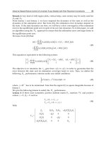
2. SISO systems with control plant of second order
Let us consider cases of two integrator blocks in series, canonical controllable form and
Jordan form. In first case we use one of the catastrophe functions, and in other two cases we
offer our own two nonlinear functions as the controller.
2.1 Two integrator blocks in series
Let us suppose that control plant is presented by two integrator blocks in series (Fig. 1) and
described by equations (2.1)


u x
2

x
1
=y
ST
2
1
ST
1
1


Fig. 1.

Robust Stabilization by Additional Equilibrium

5

1
2
1
2
2
1
1
,
.
dx
x
dt T
dx

u
dt T









(2.1)
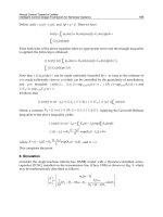
Let us use one of the catastrophe function as controller:



3222
2211122231
3ux xxkxx kxkx      , (2.2)
and in order to study stability of the system let us suppose that there is no input signal in
the system (equal to zero). Hence, the system with proposed controller can be presented as:


1
2
1
3222
2
2211122231
2

1
1
3
,
.
dx
x
dt T
dx
x xxkxx kxkx
dt T






   




1
y
x

. (2.3)
The system (2.3) has following equilibrium points

1

1
0
s
x

,
1
2
0
s
x

; (2.4)

2
3
1
1
s
k
x
k

,
2
2
0
s
x


. (2.5)
Equilibrium (2.4) is origin, typical for all linear systems. Equilibrium (2.5) is additional,
generated by nonlinear controller and provides stable motion of the system (2.3) to it.
Stability conditions for equilibrium point (2.4) obtained via linearization are

2
2
3
12
0
0
,
.
k
T
k
TT










(2.6)
Stability conditions of the equilibrium point (2.6) are

22
321
2
12
3
12
3
0
0
,
.
kkk
kT
k
TT











(2.7)
By comparing the stability conditions given by (2.6) and (2.7) we find that the signs of the
expressions in the second inequalities are opposite. Also we can see that the signs of
expressions in the first inequalities can be opposite due to squares of the parameters

k
1
and
k
3
if we properly set their values.

Recent Advances in Robust Control – Novel Approaches and Design Methods

6
Let us suppose that parameter T
1
can be perturbed but remains positive. If we set k
2
and k
3

both negative and
2
3
2
2
1
3
k
k
k
 then the value of parameter T
2
is irrelevant. It can assume any

values both positive and negative (except zero), and the system given by (2.3) remains
stable. If
T
2
is positive then the system converges to the equilibrium point (2.4) (becomes
stable). Likewise, if
T
2
is negative then the system converges to the equilibrium point (2.5)
which appears (becomes stable). At this moment the equilibrium point (2.4) becomes
unstable (disappears).
Let us suppose that
T
2
is positive, or can be perturbed staying positive. So if we can set the k
2

and
k
3
both negative and
2
3
2
2
1
3
k
k
k

 then it does not matter what value (negative or
positive) the parameter
T
1
would be (except zero), in any case the system (2) will be stable. If
T
1
is positive then equilibrium point (2.4) appears (becomes stable) and equilibrium point
(2.5) becomes unstable (disappears) and vice versa, if
T
1
is negative then equilibrium point
(2.5) appears (become stable) and equilibrium point (2.4) becomes unstable (disappears).
Results of MatLab simulation for the first and second cases are presented in Fig. 2 and 3
respectively. In both cases we see how phase trajectories converge to equilibrium points

00,
and
3
1
0;
k
k




In Fig.2 the phase portrait of the system (2.3) at constant
k
1

=1, k
2
=-5, k
3
=-2, T
1
=100 and
various (perturbed)
T
2
(from -4500 to 4500 with step 1000) with initial condition x=(-1;0) is
shown. In Fig.3 the phase portrait of the system (2.3) at constant
k
1
=2, k
2
=-3, k
3
=-1, T
2
=1000
and various (perturbed)
T
1
(from -450 to 450 with step 100) with initial condition x=(-0.25;0)
is shown.


Fig. 2. Behavior of designed control system in the case of integrators in series at various
T

2
.

Robust Stabilization by Additional Equilibrium

7

Fig. 3. Behavior of designed control system in the case of integrators in series at various
T
1
.
2.2 Canonical controllable form
Let us suppose that control plant is presented (or reduced) by canonical controllable form:
1
2
2
21 12
,
.
dx
x
dt
dx
ax ax u
dt








 




1
y
x

(2.8)
Let us choose the controller in following parabolic form:

2
11 21
ukxkx  (2.9)
Thus, new control system becomes nonlinear:
1
2
2
2
21 12 11 21
,
.
dx
x
dt
dx
ax ax kx kx

dt






   




1
y
x

. (2.10)
and has two following equilibrium points:

1
1
0
s
x

,
1
2
0
s

x

; (2.11)

2
22
1
1
s
ka
x
k

 ,
2
2
0
s
x

; (2.12)

Recent Advances in Robust Control – Novel Approaches and Design Methods

8
Stability conditions for equilibrium points (2.11) and (2.12) respectively are
1
22
0,
.

a
ak







1
22
0,
.
a
ak






Here equlibrium (2.12) is additional and provides stability to the system (2.10) in the case
when k
2
is negative.
2.3 Jordan form
Let us suppose that dynamical system is presented in Jordan form and described by
following equations:

1

11
2
22
,
.
dx
x
dt
dx
x
dt











(2.13)
Here we can use the fact that states are not coincided to each other and add three
equilibrium points. Hence, the control law is chosen in following form:

2
111
ab
ukxkx  ,

2
222
ac
ukxkx  (2.14)
Hence, the system (2.13) with set control (2.14) is:

2
1
11 1 1
2
2
22 2 2
,
.
ab
ac
dx
xkx kx
dt
dx
xkxkx
dt












(2.15)
Totaly, due to designed control (2.14) we have four equilibria:

1
1
0
s
x

,
1
2
0
s
x

; (2.16)

2
1
0
s
x

,
2
2

2
c
s
a
k
x
k


 ; (2.17)

3
1
1
b
s
a
k
x
k


 ,
3
2
0
s
x

; (2.18)

4
1
1
b
s
a
k
x
k



,
4
2
2
c
s
a
k
x
k


 ; (2.19)
Stability conditions for the equilibrium point (2.16) are:

Robust Stabilization by Additional Equilibrium

9
1
2
0
0
,
.
b
c
k
k










Stability conditions for the equilibrium point (2.17) are:
1
2
0
0
,
.
b
c

k
k










Stability conditions for the equilibrium point (2.18) are:
1
2
0
0
,
.
b
c
k
k











Stability conditions for the equilibrium point (2.19) are:
1
2
0
0
,
.
b
c
k
k










These four equilibria provide stable motion of the system (2.15) at any values of unknown
parameters 
1
and 
2
positive or negative. By parameters k

a
, k
b
, k
c
we can set the coordinates
of added equilibria, hence the trajectory of system’s motion will be globally bound within a
rectangle, corners of which are the equilibria coordinates (2.16), (2.17), (2.18), (2.19)
themselves.
3. Applications
3.1 Unknown stiffness in mass-damper-spring system
Let us apply our approach in a widely used academic example such as mass-damper-spring
system (Fig. 4).


Fig. 4.
The dynamics of such system is described by the following 2nd-order de
ferential equation,
by Newton’s Second Law
mx cx kx u


 
, (3.1)
where x is the displacement of the mass block from the equilibrium position and F = u is the
force acting on the mass, with m the mass, c the damper constant and k the spring constant.

Recent Advances in Robust Control – Novel Approaches and Design Methods

10

We consider a case when k is unknown parameter. Positivity or negativity of this parameter
defines compression or decompression of the spring. In realistic system it can be unknown if
the spring was exposed by thermal or moisture actions for a long time. Let us represent the
system (3.1) by following equations:


12
212
11
,
.
xx
xkxcxu
mm




 




(3.2)
that correspond to structural diagram shown in Fig. 5.


Fig. 5.
Let us set the controller in the form:

2
1
u
ukx , (3.3)
Hence, system (3.2) is transformed to:


12
2
2121
11
,
.
u
xx
xkxcxkx
mm




 




(3.4)
Designed control system (3.4) has two equilibira:

1

0x

,
2
0x

; (3.5)
that is original, and

1
u
k
x
k
 ,
2
0x

. (3.6)
that is additional. Origin is stable when following conditions are satisfaied:

0
c
m

,
0
k
m


(3.7)
This means that if parameter k is positive then system tends to the stable origin and
displacement of x is equal or very close to zero. Additional equilibrium is stable when

0
c
m

,
0
k
m

(3.8)

Robust Stabilization by Additional Equilibrium

11
Thus, when k is negative the system is also stable but tends to the (3.6). That means that
displacement x is equal to
u
k
k
and we can adjust this value by setting the control parameter k
u
.
In Fig. 5 and Fig. 6 are presented results of MATLAB simulation of behavior of the system
(3.4) at negative and positive values of parameter k.

Fig. 6.

Fig. 7.
In Fig. 6 changing of the displacement of the system at initial conditions x=[-0.05, 0] is
shown. Here the red line corresponds to case when k = -5, green line corresponds to k = -4,
blue line corresponds to k = -3, cyan line corresponds to k = -2, magenta line corresponds to
k = -1. Everywhere the system is stable and tends to additional equilibria (3.6) which has
different values due to the ratio
u
k
k
.
In Fig. 7 the displacement of the system at initial conditions x=[-0.05, 0] tends tot he origin.
Colors of the lines correspond tot he following values of k: red is when k = 1, green is when
k = 2, blue is when k = 3, cyan is when k = 4, and magenta is when k = 5.

Recent Advances in Robust Control – Novel Approaches and Design Methods

12
3.2 SISO systems of high order. Center of oscillations of ACC Benchmark
Let us consider ACC Benchmark system given in MATLAB Robust Toolbox Help. The
mechanism itself is presented in Fig. 8.


Fig. 8.
Structural diagram is presented in Fig. 9, where
1
2
1
1
G

ms
 ,
2
2
2
1
G
ms
 .


Fig. 9.
Dynamical system can be described by following equations:

12
213
22
34
41
111
1
,
,
,
.
xx
kk
xxx
mm
xx

kk
xx u
mmm




 














(3.9)
Without no control input the system produces periodic oscillations. Magnitude and center
of the oscillations are defined by initial conditions. For example, let us set the parameters of
the system k = 1, m
1
= 1, m
2
= 1. If we assume initial conditions x = [-0.1, 0, 0, 0] then center

of oscillations will be displaced in negative (left) direction as it is shown in Fig. 10a. If initial
conditions are x = [0.1, 0, 0, 0] then the center will be displaced in positive direction as it is
shown in Fig. 10b.
After settting the controller

Robust Stabilization by Additional Equilibrium

13

2
111
ux kx
, (3.10)
and obtaining new control system


12
213
22
34
2
41 11
111
1
,
,
,
.
u
xx

kk
xxx
mm
xx
kk
xx xkx
mmm




 






 







(3.11)
we can obtain less displacement of the center of oscillations.

Fig. 10.a Fig. 10.b
Fig. 10.
In Fig. 11 and Fig.12 the results of MATLAB simulation are presented. At the same
parameters k = 1, m
1
= 1, m
2
= 1 and initial conditions x = [-0.1, 0, 0, 0], the center is ‘almost‘
not displaced from the zero point (Fig. 11).


Fig. 11.