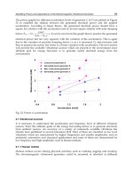
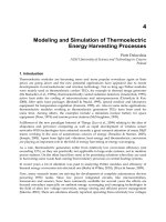
Sustainable Energy Harvesting Technologies Past Present and Future Part 5 pptx

Modelling Theory and Applications of the Electromagnetic Vibrational Generator

69
If the magnetic field B is constant with the position x then,
BlIF
em
=
where l is the coil
mean length.
In this chapter we will present the magnetic flux density (B) varies with the coil movement,
so that
2
()
1
()()()
em
cl cl cl
d
Vd ddxd dx
dx
F
RR
j
Ldx R R
j
Ldx dt dx R R
j
Ldt
φ
φφφ

ωω ω
== =
++ ++ ++

where, V is the generated voltage, R
c
is the coil resistance, L is the coil inductance, and R
l
is
the load resistance.
For an N turn coil, the total flux linkage gradient would be the summation of the individual
turns flux linkage gradients. If the flux linkage gradient for each turn is equal then the
electromagnetic force is given by;
dt
dx
D
dt
dx
LjRR
dx
d
N
F
em
lc
em
=
++
=
ω

φ
22
)(

Where the electromagnetic damping,

lc
em
RLjR
dx
d
N
D
++
=
ω
φ
22
)(
(15)
It can be seen from (15) that electromagnetic damping can be varied by changing the load
resistance R
c
, the coil parameters (N, R
c
and L), magnet dimension and hence flux (
φ
) and
the generator structure which influence
dx

d
φ
. Putting the electromagnetic force
(
dt
dx
DF
emem
=
) in equation (7) gives;

tFkx
dt
dx
D
dt
dx
D
dt
xd
m
emp
ω
sin
0
2
2
=+++
(16)
The solution of equation (9) defines the displacement under electrical load condition and is

given by the following equation,

22
0
])[()(
)sin(
ωω
θω
emp
load
DDmk
tF
x
++−
−
=
(17)
Where
]
)(
)(
[tan
2
1
ω
ω
θ
mk
DD
emp

−
+
=
−

The displacement at resonance under load is therefore given by;

Sustainable Energy Harvesting Technologies – Past, Present and Future

70

ω
ω
)(
cos
0
emp
load
DD
tF
x
+
−
=
(18)
1.5.1 Generated mechanical power
The instantaneous mechanical power associated with the moving mass under the electrical
load condition is
)().()( tUtFtP
mech

=

dt
dx
tF
load
)sin(
0
ω
=


)(
)(sin
22
0
emp
DD
tF
+
=
ω
using equation (18)
Where F(t) and U(t) are the applied sinusoidal force and velocity of the moving mass,
respectively, due to the sinusoidal movement. This corresponds to maximum mechanical
power when D
em
=0 , i.e. at no load.
The average mechanical power is defined by,
∫

+
=
T
emp
mech
dt
DD
tF
T
P
0
22
0
)(
)(sin
1
ω

)(2
2
0
emp
DD
F
+
=

1.5.2 Generated electrical power and optimum damping condition
In a similar manner, the generated electrical power can be obtained from;
)()(.)(

2
tUDtUFtP
ememe
==

The average electrical power can be obtained from,

dt
d
t
dx
D
T
P
load
eme
2
)(
1
∫
=
(19)
Taking the time derivative of equation (10) and putting the value in equation (12), we obtain

])()[(2
)(
2222
2
0
ωω

ω
emp
eme
DDmk
F
DP
++−
=
(20)
The average electrical power generated at the resonance condition (ω=ω
n
) is given by ;

2
2
0
)(2
emp
eme
DD
F
DP
+
=
(21)
If the parasitic damping is assumed to be constant over the displacement range then the
maximum electrical power generated can be obtained for the optimum electromagnetic

Modelling Theory and Applications of the Electromagnetic Vibrational Generator

71
damping. At the resonance condition (ω=ω
n
), the maximum electrical power and optimum
electromagnetic damping can be found by setting
em
e
dD
dP
=0 and solving for D
em
. This gives
the maximum power as;

p
D
F
P
8
2
0
max
=
(22)
This occurs when
pem
DD
=
, which is the optimum electromagnetic damping at the
resonance condition. Putting the value

pem
DD
=
in equation (8) gives the displacement at
the optimum load.

2
loadno
load
x
x
−
=
(23)
Thus, at the resonance condition, maximum power will be generated when the load
displacement is half of the no-load displacement.
1.5.3 Maximum power and maximum efficiency
The maximum efficiency and maximum power depends on the external driving force and
the design issues of the electromagnetic generators. If the driving force is fixed over the
variation of the load and the electromagnetic damping or force factor (Bl) is significantly
high compare to mechanical damping factor then the maximum power and maximum
efficiency will appear at the same load resistance. Otherwise when the driving force is not
constant and the force factor is significantly low or not high enough compare to mechanical
damping or any of these situations the maximum power and the maximum efficiency will
occur on different load resistance values.
1.5.4 Optimum load resistance for maximum generated electrical power
It is always desirable to operate the device at high efficiency and for an electrical generator,
it is also desired to deliver maximum power to the load at a relatively high voltage. In an
electromagnetic generator, most of the electrical power loss appears due to the coil’s internal
resistance. Here we will investigate what would be the optimum load resistance in order to

get maximum power to the load. The electrical power and voltage lost in the coil internal
resistance under these conditions are also investigated.
The optimum power condition occurs for
pem
DD =
, which can be written as,
p
lc
D
LjRRdx
d
N =
++
ω
φ
1
)(
22

In general, for less than 1 kHz frequency,
Lj
ω
can be neglected compared to R
c
.Therefore,
rearranging to get R
l
, gives the optimum load resistance which ensures maximum generated
electrical power namely,

Sustainable Energy Harvesting Technologies – Past, Present and Future

72

c
p
l
R
D
dx
d
N
R −=
22
)(
φ
(24)
The above equation indicates that an optimum load resistance may not be positive if the first
term on the right side is less than R
c
. This can occur if either the parasitic damping factor
(D
p
) is large, the flux linkage gradient (
dx
d
φ
) is low, or the coil resistance is high. Since it is
therefore not always possible to achieve the optimum condition by adjusting the load
resistance, then it is worth considering the optimum conditions in various situations.

Very Low Electromagnetic damping case (Dem<<Dp) :
In the low electromagnetic damping case, due to low
dx
d
φ
or high R
c
, it is impossible to
make the electromagnetic damping equal to the parasitic damping. If the electromagnetic
damping for the short circuit condition is much less than the parasitic damping (D
em
<<D
p
),
there will be no significant change in displacement between the no-load and load
conditions. In this case, the maximum power will be delivered to the load when the load
resistance is matched to the coil resistance. Since the load resistance has to be equal to the
generator internal resistance, 50% of the voltage and power will be lost in the generator
internal resistance and the generator efficiency is likely to be very low.
Limitation of the model ( D
p
< D
em
<D
p
) :
If the electromagnetic damping for very low load resistance is only slightly less than D
p
, but
can not be made equal to D

p
then there will be a change in displacement between the no-
load and load condition but the optimum load resistance at maximum generated power
condition cannot be analyzed by the modeling equation. However, the optimum load
resistance to maximize the load power condition, as opposed to the generated power could
be determined from the modeling equation.

1.5.5 Optimum load resistance for maximum load power
In order to find the optimum resistance which maximizes the load power, we can take the
expression for the load power and differentiate with respect to the load resistance.
The average generated electrical power is:
2
2
0
)(2
emp
eme
DD
F
DP
+
=

The average load power would therefore be:
]
)(2
[
2
2
0

emp
em
lc
l
load
DD
FD
RR
R
P
+
+
=

Inserting the expression for D
em
from equation (15) and rearranging gives:

Modelling Theory and Applications of the Electromagnetic Vibrational Generator

73
222
222
])()([2
)(
N
dx
d
RRD
dx

d
NFR
P
lcp
ol
load
φ
φ
++
=

Now the optimum load resistance at the maximum load power can be found by setting
0=
l
l
dR
dP
, which gives:

p
clopt
D
dx
d
N
RR
22
)(
φ
+=

(25)
In order to understand the optimum conditions of the generators, the displacement and load
power were calculated theoretically for different parasitic damping factors. The parasitic
damping, EM damping, displacement, generated voltage, the load power and the optimum
load resistance at maximum load power were calculated by the following equations using
the values in Table 1;
oc
n
p
Q
m
D
ω
=
,
lc
em
RR
dx
d
ND
+
=
2
2
)(
φ
,
nemp
load

DD
ma
x
ω
)( +
=
,
dt
dx
dx
d
V
φ
=
,
2
2
)(2
)(
lcl
l
l
RRR
VR
P
+
=
,
p
clopt

D
dx
d
N
RR
22
)(
φ
+=


Parameters value
N 500
Coil internal resistance, R
c
(Ω)
33
Flux linkage gradient,
dx
d
φ
(wb/m)
1e-03
Frequency, f (Hz) 1000
Acceleration, a (m/s
2
) 9.81
Mass (kg) 1.97e-03
Table 1. Assumed parameters of the Generators
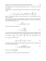
Figure 13 shows the displacement vs load resistance, assuming different values of open

circuit quality factor (Q
oc
) for a 500 turns coil. It can be seen from the graphs that the
significant variation of displacement for Qoc =10000 (Dp=0.0012 N.s/m) is due to the change
in the load resistance value. Figures 14, 15 and 16 show the corresponding load power and
damping factor vs load resistance. For Qoc=10000, the maximum power is generated and

Sustainable Energy Harvesting Technologies – Past, Present and Future

74
transferred to the load when the electromagnetic damping is equal to the parasitic damping;
this agrees with the theoretical model. In this case, the electromagnetic damping for very
low load resistance is almost 6 times higher (D
em
>>D
p
) than the parasitic damping factor.
Since the optimum R
load
is much greater than R
coil
, 90% of the generated electrical power is
delivered to the optimum load resistance value. The optimum load resistance at maximum
load power is 255
Ω, which agrees with the theoretical equation (25).
For Qoc=1000 there is some variation of displacement for changing load resistance values
but it is not as significant as for the Qoc=10000 case. In this case, electromagnetic damping
for low load resistance is lower than parasitic damping (D
em
< D

p
) but not significantly lower.
In this situation the optimum condition for the generated maximum power could not be
defined by the modeling equation but the optimum load resistance at maximum load power
is 55 which agrees well with theoretical equation (25). The optimum load resistance tends to
be close in value to the coil resistance.

0
0.5
1
1.5
2
2.5
1 10 100 1000 10000
Load resistance (ohm)
Calculated displacement (mm)
Displacement- Qoc=10000
Displacement - Qoc=1000
Displacement -Qoc=200

Fig. 13. Variation of displacement for different quality factors for N =500 turns coil generator
For Qoc=200, there is no variation of displacement for changing load resistance values and
the electromagnetic damping for all load resistances is significantly lower than the parasitic
damping factor (D
p
>>D
em
). In this case the maximum power is delivered to the load when
the load resistance equals the coil resistance. It is assumed in the above that the parasitic
damping is almost constant with the displacement. However, this parasitic damping can

depend on the generator structure and the properties of the spring material such as friction,
material loss etc.

Modelling Theory and Applications of the Electromagnetic Vibrational Generator

75
0
7
14
21
28
35
10 100 1000 10000
Load resistance (ohm)
Load power (mW)
0.000
0.002
0.003
0.005
0.006
0.008
Damping factor (N.s/m)
Load power- Qoc=10000
Parasitic damping
EM damping

Fig. 14. Calculated load power and damping factor for Qoc= 10000 and N=500 turns coil
generator.
0
0.4

0.8
1.2
1.6
1 10 100 1000 10000
Load resistance (ohm)
Load power (mW)
0.00001
0.0001
0.001
0.01
0.1
Damping factor (N.s/m)
Load power - Qoc=1000
Parasitic damping
EM damping

Fig. 15. Calculated load power and damping factor for Q
oc
= 1000 and N=500 turns coil
generator.

Sustainable Energy Harvesting Technologies – Past, Present and Future

76
0
0.02
0.04
0.06
0.08
0.1

1 10 100 1000 10000
Load resistance (ohm)
Load power (mW)
0
0.013
0.026
0.039
0.052
0.065
Damping factor (N.s/m)
Load power - Qoc=200
Parasitic damping
EM damping

Fig. 16. Calculated load power and damping factor for Q
oc
= 200 and N=500 turns coil
generator.
1.6 Parasitic or mechanical damping and open circuit quality factor
The parasitic damper model of the mechanical beam in the electromagnetic vibrational
generator structure is considered as a linear viscous damper [22-27]. The parasitic damping
therefore determines the open-circuit or un-loaded quality factor which can be expressed as;


12
2
1
ff
f
D

m
Q
n
pp
n
p
−
===
ς
ω
(26)
Where
p
ς
is the parasitic damping ratio, f
1
is is the lower cut-off frequency, f
2
is the upper
cut-off frequency and f
n
is the resonance frequency of the power bandwidth curve which is
shown in graph 17. The quality factor can also be calculated from the voltage decay curve or
displacement decay curve for the system when subjected to an impulse excitation, according
to equation [22]:
)ln()ln(
2
1
2
1

V
V
tf
x
x
tf
Q
nn
p
Δ
=
Δ
=
ππ

In general, the unloaded quality factor of a miniature resonant generator is influenced by
various factors. At its most general, it can be expressed as:

1
11111
−
⎟
⎟
⎠
⎞
⎜
⎜
⎝
⎛
++++=

fsuctm
p
QQQQQ
Q
(27)

Modelling Theory and Applications of the Electromagnetic Vibrational Generator

77
where 1/Q
m
is the dissipation arising from the material loss, 1/Q
t
is the dissipation arising from
the thermoelastic loss, 1/Q
c
is the dissipation arising from the clamping loss, 1/Q
su
is the
dissipation arising from the surface loss, and 1/Q
f
is the dissipation arising from the
surrounding fluid. There have been considerable efforts to find analytical expressions for these
various damping mechanisms, particularly for Silicon-based MEMS devices such as
resonators. However further analysis of the parasitic damping factor is beyond in this chapter.

Fig. 17. Power bandwidth curve
1.7 Spring constant (k) of a cantilever beam
A cantilever is commonly defined as a straight beam, as shown in Figure 18 with a fixed
support at one end only and loaded by one or more point loads or distributed loads acting

perpendicular to the beam axis. The cantilever beam is widely used in structural elements
and the equations that govern the behavior of the cantilever beam with a rectangular cross
section are simpler than other beams. This section shows the equations that the maximum
allowable vertical deflection, the natural frequency and spring constant due to the end
loading of the cantilever.
The maximum allowable deflection the spring can tolerate is [27]:

max
2
max
3
2
σ
Et
L
y =
(28)
where
max
σ
is the maximum stress, E is Young’s modulus, t is the thickness of the
cantilever, and L is the length of the cantilever.
The maximum stress can be defined as
max
2
FLt
I
σ
= where F is the vertical applied force and
12

3
Wt
I =
is the moment of inertia of the
beam.
0.4
0.55
0.7
0.85
1
612182430
Frequency (Hz)
Vibration amplitude(m)
f
1
f
n
f
2

Sustainable Energy Harvesting Technologies – Past, Present and Future

78
The ratio between the force and the deflection is called the spring constant, k and is given
by:

3
3
L
EI

k =
(29)
The
total end mass of the beam is m = 0.23M +m
1

where m
1
is the added mass and M is the mass of cantilever.
The equation of motion for free undamped vibration is:
0
2
2
=+
∂
∂
ky
t
y
m
, where, m is the total end mass of the beam. If
tAy
n
ω
cos
=
then the
natural frequency would be,

m

k
f
n
π
2
1
=
(30)
The next section presents the electrical circuit analogy of the electromagnetic vibrational
generator.

Fig. 18. Cantilever beam deflection
1.8 Equivalent electrical circuit of electromagnetic vibrational generator
The vibrational generator consists of mechanical and electrical components. The mechanical
components can be easily represented by the equivalent electrical circuit model using any
electrical spice simulation software in order to understand their interactions and behaviours.
Two possible analogies either impedance analogy or mobility analogy is normally used in
the transducer industry which compare mechanical to electrical systems. However it is good
idea to use the analogy that allows for the most understanding and also it is easy to switch
one analogy to other. Table 2 [29-30] shows the equivalent electrical circuit elements of the

Modelling Theory and Applications of the Electromagnetic Vibrational Generator

79
mechanical components for the electromagnetic vibrational generator. Figure 19 shows the
equivalent electrical circuit of the force driven electromagnetic linear or vibrational
generator. When an external force (F) is applied to the generator housing or diaphragm the
voltage will be generated at the coil terminal due to the relative displacement between
magnet and coil. The moving mass, mechanical compliance, mechanical resistance, coil
resistance, coil inductance, load resistance and the force factor of the alternator are M

m
, C
m
=
1/k, R
m
, R
c
, L
c
, R
L
and Bl respectively.

Mechanical elements
Equivalent Electrical elements
Impedance analogy Mobility analogy
Force (F) Voltage (E) Current (I)
Velocity (U) Current (I) Voltage (E)
Mechanical resistance (R
m
) Resistance (R) Conductance (G)
Mechanical mass (M) Inductance (L) Capacitance (C)
Mechanical compliance (C
m
) Capacitance (C ) Inductance (L)
Table 2. Electrical equivalent of the mechanical components.

Fig. 19. Equivalent electrical circuit of the electromagnetic vibrational generator.
2. Verification of the model

In order to verify the model and the optimization theory several macro generators had been
built and tested using a controllable shaker during Author’s Ph.D study. Some of these
works have already been highlighted in literatures [6]. It was important to vibrate the
generator exactly at resonance in order to observe the electromagnetic damping effect for
different load conditions. If the vibration frequency is far away from the system’s resonant
frequency, then the damping would not have any significant effect on displacement since
the displacement is mainly controlled by the spring constant at off resonance. All the
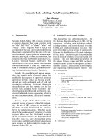
prototypes which have been built and tested consisted of four magnets (NdFeB35) with a
wire-wound copper coil placed between the magnets as shown in Figure 20. The advantages
of the four magnet generator structure have already been described in the previous section.
Table 3 gives the coil and magnet parameters for macro generator A and B. The generators
were vibrated using a sinusoidal acceleration with the frequency matched to the generator’s
mechanical resonant frequency.

Sustainable Energy Harvesting Technologies – Past, Present and Future

80

Fig. 20. Generator A-showing four magnets attached to a copper beam and wire-wound coil.

Parameters Generator -A Generator-B
Moving mass (kg) 0.0428 0.025
Magnet size (mm) 15 x 15 x 5 10 x 10 x 3
Resonant frequency (Hz) 13.11 84
Acceleration (m/s
2
) 0.78 7.8
Magnet and coil gap (mm) 1.25 1.5
Coil outer diameter (mm) 28.5 13.3
Coil inner diameter (mm) 5 2

Coil thickness (mm) 7.5 7
Coil turns 850 300
Coil resistance (ohm) 18 3.65
Table 3. Generator Parameters.
Measured and calculated results of the macro-generator A & B
The displacement and voltage were measured for various load resistances. The load power
is calculated from the voltage and load resistance. The parasitic damping can be calculated
using the no-load displacement equation:
ω
ω
p
loadno
D
tF
x
cos
−
=
−
,
ω
loadno
p
x
F
D
−
=
0

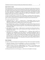
The generators were also simulated using a 3-D finite element (FE) transient model with the
measured displacement as input. Figure 21 shows the half model of the generator structure
used in the FE model and the simulated flux linkage vs displacement of macro generator A

Modelling Theory and Applications of the Electromagnetic Vibrational Generator

81
& B. The simulated flux linkage gradients (
)
dx
d
φ
of the generator A and B are 0.00542 Wb/m
and 0.0013 Wb/m respectively.


(a)

-0.02
-0.01
0.00
0.01
0.02
-3 -2 -1 0 1 2 3
Displacement (mm)
Fluxlinkage (wb)
-0.002
-0.001
0.000
0.001

0.002
Fluxlinkage (wb)
Generator-A
Generator-B

(b)
Fig. 21. Simulated Generator models used in (a) FE simulation and (b) the resulting flux
linkage gradient vs displacement.
These values are used in the following equation to calculate the electromagnetic damping;
lc
em
RR
dx
d
N
D
+
=
22
)(
φ


Sustainable Energy Harvesting Technologies – Past, Present and Future

82
The parasitic and electromagnetic damping can then be used in the following equation to
calculate the power:
2
2

)(
emp
emavg
DD
F
DP
+
=

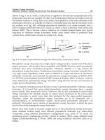
Figures 22 and 23 show the measured displacement and the measured and simulated load
voltages for different load conditions for generator-A and generator B, respectively. The
measured and simulated voltages agree quite closely. Figure 24 and 25 show the measured
and calculated power, and the estimated parasitic and electromagnetic damping, for
generators A and B, respectively. The calculated open circuit quality factors
p
n
oc
D
m
Q
ω
=
are
58.85 and 56.87 for generators A & B, respectively. The graph in Figure 22 shows that there is a
significant change in displacement with the change in load, for generator A. However for
generator B, the displacement does not vary with load. This is consistent with the fact that the
electromagnetic damping is comparable to the parasitic damping for generator A, but the
electromagnetic damping is much lower for generator B than the parasitic damping due to
larger gap between magnet and coil, and smaller magnets used. This can be seen from figure
24 and 25. Furthermore, the graph in figure 24 shows that the power readies a maximum for

the value of load resistance at which electromagnetic damping and parasitic damping are
equal. The optimum load resistance is 432 Ω, which agrees well with the theoretical equation.
For generator B, the electromagnetic damping is always much less than the parasitic damping
and the power is maximized for a load resistance equal to the coil resistance. In figure 24 there
is a small discrepancy between the measured and calculated power since the calculated power
assumes a sinusoidal voltage but the measured voltage is not exactly sinusoidal.
0
2
4
6
8
0 700 1400 2100 2800 3500
Load resistance ( ohm)
Displacement(mm
)
0
1
2
3
4
Peak load voltage(V)
Displacement
Measured load voltage
FEM voltage

Fig. 22. Measured displacement and simulated and measured load voltage for generator A.

Modelling Theory and Applications of the Electromagnetic Vibrational Generator

83

0
0.3
0.6
0.9
1.2
1.5
1 6 11 16 21
Load resistance(ohm)
Displacement(mm)
0
60
120
180
240
300
Peak load voltage(mV)
Displacement
Measured load Peak voltage
FEM load voltage

Fig. 23. Measured displacement and simulated and measured load voltage for generator B.
0
0.6
1.2
1.8
2.4
0 400 800 1200 1600 2000
Load resistance(ohm)
Load power(mW)
0

0.15
0.3
0.45
0.6
Damping factor(N.s/m)
Measured power
Calculated power
Electromagnetic damping
Parasitic damping

Fig. 24. Measured and calculated load power and estimated parasitic and electromagnetic
damping for generator A.
In order to understand the parasitic damping effect and the optimum condition of the
generator, more macro generators have been built and tested. Table 4 shows the generator

Sustainable Energy Harvesting Technologies – Past, Present and Future

84
parameters of macro generators C, D and E. Generators C, D, and E were tested for different
acceleration levels and the vibration frequency of the shaker was swept in order to
determine the resonance frequency. In generators A and B, the parasitic damping factor and
the open circuit quality factor were calculated from the measured no-load displacement.
However, for generators C, D and E, the no-load and load voltages at the half power
bandwidth frequency were measured in order to determine the open circuit and closed
circuit quality factors and hence the damping. Figures 26, 27 and 28 show the no-load
voltages for different acceleration levels of generators C, D, and E, respectively. It can be
seen from these figures that as the acceleration level increases, the resonance frequency
shifts to a lower frequency due to the spring softening characteristic of the spring constant
[31]. This indicates that the displacement of the spring constant is approaching the non-
linear region. However, the resonance frequency could also shift to a higher frequency with

increased acceleration level which is normally known as a spring hardening characteristic.
0
1
2
3
4
0 5 10 15 20 25
Load resistance(ohm)
Load power(mW)
0
0.06
0.12
0.18
0.24
Damping factor (N.s/m)
Calculated power
Measured power
Electromagnetic damping
Parasitic damping

Fig. 25. Measured and calculated load power and estimated parasitic and electromagnetic
damping for generator –B.

Parameters Generator -C Generator-D Generator-E
Movin
g
mass
(
k
g)

0.019579 0.05116 0.05116
Ma
g
net size
(
mm
)
10 x 10 x 3 15 x 15 x 5 15 x 15 x 5
Ma
g
net and coil
g
a
p

(
mm
)
3.75 3.75 3.25
Coil outer diameter
(
mm
)
19 19 28.5
Coil inner diameter
(
mm
)
115
Coil thickness

(
mm
)
6.5 6.5 7.5
Coil turns 1100 1100 850
Coil resistance (ohm) 46 46 18
Table 4. Generator parameters

Modelling Theory and Applications of the Electromagnetic Vibrational Generator

85



Fig. 26. No-load voltage vs frequency of generator – C.



0
300
600
900
1200
14.5 15 15.5 16 16.5
Frequency (Hz)
No-load peak voltage (mV)
Acceleration- 0.15g
Acceleration - 0.097g
Acceleration- 0.07g
Change of resonance

frequency

Fig. 27. No-load voltage vs frequency for generator-D.
0
300
600
900
1200
25 25.3 25.6 25.9 26.2
Frequency (Hz)
No-load peak voltage (mV)
Acceleration - 0.1 g
Acceleration - 0.164g
Acceleration- 0.2g
Change of resonance
frequency

Sustainable Energy Harvesting Technologies – Past, Present and Future

86

Fig. 28. No-load voltage vs frequency for generator-E.
This non-linear mass, damper and spring vibration can be defined by the standard Duffing
oscillator model [31] using the following equation;

tFxkkx
dt
dx
D
dt

xd
m
ω
sin
3
3
2
2
=+++
(31)
It can be seen in the above equation that a cubic nonlinear stiffness term (k
3
x
3
) has been
added to the linear mass, damper, and spring equation. If the non–linear stiffness constant
(k
3
) is greater than zero then the model would represent a hardening spring constant. In this
case, the resonance frequency would be shifted to the right (increase) from the linear
resonance frequency with increased vibrational force, as shown in Figure 29 (a). If k
3
is less
than zero, then the model would represent a softening spring constant. In this case, the
linear resonance frequency would be shifted to the left (decrease) from the linear resonance
frequency with increased vibrational force, as shown in Figure 29 (b).
Table 5 shows the calculated open circuit quality factor, parasitic damping factor, optimum
load resistance, measured generated electrical power and load power on the optimum load
resistance of each generator for different accelerations. The open circuit quality factor and
the parasitic damping were calculated using the following formulas;

12
ff
f
Q
n
oc
−
=
,
oc
n
p
Q
m
D
ω
=

The displacements of the generators for each load were calculated according to the
equation;
200
450
700
950
1200
14.9 15.1 15.3 15.5 15.7
Frequency (Hz)
No-load peak voltage (mV)
Acceleration- 0.07g
Acceleration - 0.097g

Change of resonance
frequency

Modelling Theory and Applications of the Electromagnetic Vibrational Generator

87
nemp
load
DD
F
x
ω
)( +
=



Fig. 29. Amplitude response of (a) non linear hardening spring constant (b) non linear
softening spring constant.

Generator –C
Accelerati
on (g)
Q
oc

X
no-
load(mm)
D

p

(N.s/m)
Rc
(Ω)
R
lopt

(Ω)

D
em
@
R
lopt
Generated
electrical
power (mW)
Max. load
power
(mW)
0.10 86 3.21 0.036 46 100 0.012 0.95 0.65
0.16 67 4.16 0.046 46 75 0.019 1.90 0.95
0.20 59 4.49 0.052 46 75 0.019 2.28 1.14
Generator –D
0.07 40 2.99 0.122 46 75 0.065 1.34 0.83
0.10 36 3.76 0.133 46 75 0.065 2.23 1.38
0.15 29 4.69 0.166 46 75 0.065 3.20 1.98
Generator –E
0.07 38 2.96 0.13 18 75 0.105 1.53 1.24

0.097 35 4.27 0.12 18 100 0.105 3.00 2.20
Table 5. Calculated parasitic damping and measured power for optimum load resistance.
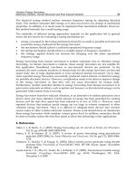
The generators were also simulated using a FE transient model in order to verify the
measured results with the simulated value. For example Figures 30 and 31 show the
measured and simulated voltages and power respectively of the generator-C for 0.1g
acceleration level. The graphs show that the measured voltages and power agree well with
the FE simulation voltages. Table 5 shows that the maximum power of generator-E are
transferred to the load when the parasitic damping equals the electromagnetic damping; this
agrees well with the theoretical model. Generator-E delivers a maximum 81% of the
generated electrical power to the load. In generator-C and D, significant electromagnetic

Sustainable Energy Harvesting Technologies – Past, Present and Future

88
damping is present but it is still not high enough to match the parasitic damping. The
optimum load resistances for all of these generators at the maximum load power agree well
with the prediction of equation (24).
It can also be seen from Table 5 that the parasitic damping is not constant for different
acceleration levels. It appears that parasitic damping increases with increasing
displacement. This parasitic damping depends on material properties, acceleration, size and
shape of the generator structure, frequency and the vibration amplitude, as has already been
explained earlier. As a consequence of this, the optimum load R
lopt
can be different for
different acceleration levels, as in the case of Generator –C.
0
1
2
3
4

0 150 300 450 600
Load resistance (ohm)
Calculated displacement (mm)
0
175
350
525
700
Load peak voltage (mV)
Displacement
Measured voltage
FE voltage

Fig. 30. Displacement and Measured and FE load voltages of generator-C for 0.1g
acceleration.
0
0.2
0.4
0.6
0.8
0 125 250 375 500
Load resistance (ohm)
Load power (mW)
0
0.01
0.02
0.03
0.04
Damping factor (N.s/m)
Measured load power

Model power
Parasitic damping
EM damping

Fig. 31. Measured and calculated load power and estimated parasitic and electromagnetic
damping of generator-C for 0.1g acceleration.