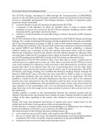
Sustainable Growth and Applications in Renewable Energy Sources Part 10 potx

Parameterisation of the Four Half-Day Daylight Situations

171

0.0 0.1 0.2 0.3 0.4 0.5 0.6 0.7 0.8 0.9 1.0
0
10
20
30
40
50
60
70
80
90
100
Pm1
Pm4
Pm2
Pm3
o
v
e
r
c
a
s
t
cl
o

ud
y
d
y
n
a
m
i
c
c
l
e
a
r

h
a
l
f
-
d
a
y
s
Probability of occurrence in %
Monthly average relative sunshine duration, s


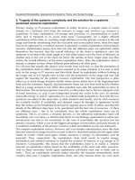
Fig. 38. Occurrence probability of half-day situations during mornings

0.0 0.1 0.2 0.3 0.4 0.5 0.6 0.7 0.8 0.9 1.0
0
10
20
30
40
50
60
70
80
90
100
Pa1
Pa4
Pa2
Pa3
o
v
e
r
c
a
s
t
c
l
o
u
d
y

d
y
n
a
m
i
c
c
l
e
a
r

h
a
l
f
-
d
a
y
s
Probability of occurrence in %
Monthly average relative sunshine duration, s


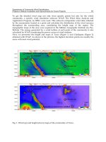
Fig. 39. Occurrence probability of half-day situations during afternoons
These probabilities of the occurrence of typical four daylight situations were derived from
measurements in two different climate zones, i.e. in Bratislava as well as in Athens. So, it can
be assumed that the dependence on monthly sunshine durations during morning and

afternoon half-days could be valid not only in Central Europe and European Mediterranean
regions but also world-wide.

Sustainable Growth and Applications in Renewable Energy Sources

172
5. Approximate redistribution of the four daylight situations in the yearly
simulation of their occurrence
In accordance with the probability study of the four daylight situations in Bratislava
morning and afternoon data during 1994-2001 the check was done using Athens data
gathered in a five year period 1992-1996 (Darula et al., 2004). Because the calculated
probability had to be substituted by a concrete number of days within a particular month,
i.e. in integer numbers, these had to correspond with sum of half-days in that actual month.
The redistribution into half-days had to dependent also on the overall monthly sunshine
duration, so the redistribution model correlating the probability percentage and number of
half-day situations had to be found. The best fit final solution is documented for the
morning redistribution model with results shown in Fig. 40 as well as for afternoon in Fig.
41 with monthly relative sunshine duration data measured during mornings sm and
measured during afternoons sa.

0.0 0.1 0.2 0.3 0.4 0.5 0.6 0.7 0.8 0.9 1.0
0.0
0.1
0.2
0.3
0.4
0.5
0.6
0.7
0.8

0.9
1.0
Five-
y
ear avera
g
e relative sunshine duration
Athens morning averages 1992-1996
Modelled sunshine duration
Bratislava morning averages 1994-2001
Redistribution model:
sm=0,92 Pm1+0,21 Pm2+0,56 Pm4
sm=(0,92 Nm1+0,25 Nm2+0,61 Nm4)/Nm

Fig. 40. Redistribution model after Bratislava and Athens morning data

0.0 0.1 0.2 0.3 0.4 0.5 0.6 0.7 0.8 0.9 1.0
0.0
0.1
0.2
0.3
0.4
0.5
0.6
0.7
0.8
0.9
1.0
Five-year average relative sunshine duration
Modelled sunshine duration

Bratislava afternoon averages 1994-2001
Athens afternoon averages 1992-1996
Redistribution model:
sa = 0,92 Pa1 + 0,05 Pa2 + 0,61 Pa4
sa = (0,9 Na1 + 0,25 Na2 + 0,5 Na4)/Na

Fig. 41. Similar redistribution for afternoon half-days

Parameterisation of the Four Half-Day Daylight Situations

173
In these figures besides the probability percentage notation 1 4Pm Pm

and 1 4Pa Pa a
similar notation for the number of half-days is used 1 4Nm Nm

and 1 4Na Na

while the
overall number of morning half-days in a particular month is Nm for mornings and Na for
afternoons in Fig. 40 and 41. These document and confirm the redistribution model that
approximates the participation of the main three situations on sunlight presence and
monthly sunshine duration within the particular half-day assuming that the overcast half-
day is absolutely without any sunshine, thus



0.92 1 0.25 2 0.61 4 /sm Nm Nm Nm Nm



, (34)
and



0.9 1 0.25 2 0.5 4 /sa Na Na Na Na


. (35)
This redistribution of half-day situations during mornings and afternoons was calculated for
Bratislava and Athens data and as examples are shown in Table 2 and 3 only those for
morning half-days. Although the verification of these redistributions for other localities is
rather complicated it is evident that the ranges of mornings
sm and those measured during
afternoons sa can be in every month specific too. While during overcast situations the range of
0.05s  is relatively small with
/
vv
GE within the spread 0.05 - 0.35 (Fig. 35 and 36), the s
ranges in dynamic situations are quite large i.e. 0.3 – 0.76 while Gv/Ev spread is
approximately within 0.32 – 0.61.
Thus eq. (34) and (35) characterise the redistribution of sm and sa due to four half-day
situations simulating Central European and Mediterranean daylight conditions. In other
climate regions (like maritime and equatorial) or during rainy (April or May) or during
monsoon months more general relations might be valid as



11 22 44/sm sm Nm sm Nm sm Nm Nm



, (36)
and



11 22 44/sa sa Na sa Na sa Na Na


. (37)
Therefore in the application of this redistribution it is recommended to test whether the sm
and sa for appropriate situations are within their usual ranges. Approximately this is done
by checking 4sm and 4sa ranges after eq. (34) and (35). During dynamic half-days both
4sm and 4sa should be in the range 0.3 to 0.75 to be related to the rise of
/
vv
GE from 0.35
to 0.6 respectively.
For an example of such a check can be taken the ten-year (1995-2004) average of relative
sunshine duration in Prague, which is for May 0.502s

. In the book by Darula et al., (2009)
after percentage probabilities the number of four half-day situations was determined (on
p. 64, Tab. 5.4.1) as follows:
18Nm  , 2 9Nm  , 3 6Nm

and 4 8Nm

with the full number of morning half-days in
May 31Nm  ;

So, after eq. (34)





31(0.502) 0.92 8 0.25 9
0.92 1 0.25 2
40.744
48
smNm Nm Nm
sm
Nm
  




Sustainable Growth and Applications in Renewable Energy Sources

174
Month s Pm1 Nm1

Pm2 Nm2

Pm3 Nm3

Pm4 Nm4

Nm sm

1 0,204 8,67 3 22,90 7 56,92 18 11,51 3 31 0,207
2 0,404 17,59 5 30,41 9 27,85 8 24,15 6 28 0,382
3 0,367 15,55 5 30,13 9 32,32 10 22,00 7 31 0,365
4 0,466 21,70 7 29,73 9 21,23 6 27,34 8 30 0,460
5 0,541 28,08 9 26,01 8 14,61 5 31,30 9 31 0,517
6 0,522 26,29 8 27,28 8 16,15 5 30,28 9 30 0,504
7 0,525 26,57 8 27,08 8 15,90 5 30,45 10 31 0,508
8 0,609 35,53 11 21,46 7 9,83 3 33,18 10 31 0,589
9 0,426 18,95 6 30,33 9 25,38 8 25,35 7 30 0,408
10 0,420 18,57 6 30,37 9 26,04 8 25,03 8 31 0,416
11 0,244 10,16 3 25,59 8 50,11 15 14,14 4 30 0,244
12 0,192 8,23 3 21,98 7 59,06 18 10,73 3 31 0,207
Table 2. Redistribution of half-day situations according to Bratislava morning 8 – year data
related to monthly average relative sunshine duration

Month s Pm1 Nm1

Pm2 Nm2

Pm3 Nm3

Pm4 Nm4

Nm sm
1 0,451 20,62 6 30,02 9 22,74 7 26,62 9 31 0,436
2 0,480 22,76 6 29,38 8 19,89 6 27,98 8 28 0,451
3 0,516 25,75 8 27,68 9 16,66 5 29,91 9 31 0,496
4 0,643 39,95 12 19,19 6 7,85 2 33,00 10 30 0,631
5 0,666 43,23 13 17,65 5 6,66 2 32,45 11 31 0,653
6 0,797 67,02 20 8,89 3 1,95 1 22,14 6 30 0,766

7 0,844 77,95 24 5,75 2 1,02 0 15,29 5 31 0,832
8 0,854 80,45 25 5,08 2 0,86 0 13,60 4 31 0,841
9 0,783 64,03 19 9,83 3 2,30 1 23,85 7 30 0,757
10 0,605 35,04 11 21,73 7 10,08 3 33,15 10 31 0,589
11 0,458 21,11 6 29,89 9 22,03 7 26,96 8 30 0,430
12 0,400 17,36 5 30,40 9 28,32 9 23,92 8 31 0,386
Table 3. Redistribution of half-day situations according to Athens morning 5 – year data
related to monthly average relative sunshine duration

Parameterisation of the Four Half-Day Daylight Situations

175
which means that sm4 = 0.744 falls to the upper range 0.75, but sm2 = 0.25 is suspect due to
probably more sunshine intervals in May. Under such conditions probably sm4 = 0.61 as in
eq. (34) and in May sm2 is higher:




31(0.502) 0.92 8 0.61 8
20.369
9
sm
  


.
Similarly a November check can be done using 0.195s

for Prague with 1 3Nm  ,

27Nm  , 3 18Nm  and 4 2Nm

with the full number of morning half-days in November
30Nm  where after eq. (34) is






30 (0.195) 0.92 3 0.25 7
0.92 1 0.25 2
40.67
42
smNm Nm Nm
sm
Nm
  




which suites the dynamic range and is quite close to the assumed sm4 = 0.61.
In accordance with the already approximated monthly averaged values
/
vv
GE
in Fig. 33,
35 and 36 as well as
/

vv
DE in Fig. 34 can be simulated also roughly half-day illuminance
courses as


sin
v
vs
v
G
G LSC
E


lx, (38)
where

23
/ 0.182 1.038 1.385 0.883
vv
GE s s s  
-, (39)
and


sin
v
vs
v
D

DLSC
E


lx, (40)
where

23
/ 0.182 0.693 0.759 0.126
vv
DE s s s  
-. (41)
It is evident that the course distribution of illuminances is caused by the sine of the solar
angle with either the momentary sine value for the moment or for the chosen time interval.
This sine of the solar altitude

s
after eq. (2) for any hour number H during daytime in
TST can be used. For a short time period a straight-line interpolation can be applied when


12
/2HHH
or a value after eq. (16) is more precise.
A further possible step to specify the site and situation dependent illuminance stimulated a
study that would show the relation of the four situations on typical sky patterns or ISO
(2004)/CIE (2003) standard general skies if possible. Originally these standards were
derived with the specification of indicatrix and gradation function in Kittler (1995) and
finally recommended for standardisation in Kittler et al., (1997).
After a detail number of 5-minute measured cases in Bratislava specifying every year within the

five year 1994 - 1998 span all four daylight situations were analysed with the following results:
1.
under situation 1 were present
-
during mornings over 75% of clear sky types 11, 12 and 13 with the prevailing 32.55 %
of sky type 12,

Sustainable Growth and Applications in Renewable Energy Sources

176
- during afternoons over 76 % sky types 10, 11 and 12 with the prevailing 34.48 % of sky
type 12,
2.
under situation 2 were occurring
-
during mornings almost 50% of cloudy sky types 2, 3 and 4 with the prevailing 18 % of
sky type 3,
-
during afternoons over 46 % sky types 2, 3 and 4 with the prevailing almost 17 % of sky
type 3,
3.
under situation 3 were present
-
during mornings almost 72% of overcast sky types 1, 2, and 3 with the prevailing
almost 27 % of sky type 2,
-
during afternoons over 70 % sky types 1, 2, and 3 with the prevailing almost 27 % of sky
type 2,
4.
under sitation 4 were very changeable sky patterns, but the most present were

-
during mornings almost 40 % sky types 11, 12 and 13 with the prevailing over 15 % of
sky type 12,
-
during afternoons almost 38 % sky types 11, 12 and 13 with the prevailing almost 15%
of sky type 12.
This sky type prevalence (Darula & Kittler, 2008a) was in coherence considerably also with
the seasonal frequency of dominant sky types found in the seasonal distribution (Kitttler et
al., 2001) with prevailing overcast skies in type 2 and 3 and clear sky types 12 and 11 in
Bratislava, while in Athens the highest frequency of clear polluted sky type 13 was
documented, while uniform cloudy skies 5 and 6 were the most often occurring in dull
seasons. Of course, the seasonal changes in occurrence frequency of clear and overcast skies
is linked with relative sunshine duration and therefore with the number of half-days in any
locality. However, it is interesting that in any daylight climate there exists a number of
(Lambert) overcast sky type 5 with uniform luminance sky patterns, e.g. in Bratislava five
year long-term these represented 12.6 % whithin cloudy situation 2 during morning half-
days and over 14 % during afternoons whithin overcast situation 3 these were represented
by morning 8.08 % and afternoon 7.74 % presence.
More and further measurements in different locations are expected to demonstrate the site-
specific and short-term variability of illuminance levels (as recently was shown for
irradiance by Perez et al., 2011). Due to dynamic situations it is important to evaluate short-
term (momentary 1 or 5-minute regular measurements) because estimations of using hourly
insolation data from satellite-based sources can be problematic and less accurate when
subhourly variability is uncertain and especially if irradiance data are recalculated via
luminous efficacy into illuminances (Darula & Kittler, 2008b). Therefore long-term regular
measurements in absolute illuminance values are so important to have site-specific
fundamental data with the possibility to derive also half-day situations. When modelling
year-round situation frequencies it is also important to randomly distribute also some
sequential ocurrence of specific situations (Darula & Kittler 2002) which can occur several
half-days or even days after each other as is documented in Table 4 and 5. Of course, one

situation can last during the whole day, i.e. the morning situation is the same in the
afternoon, but quite frequent are also changes from clear to dynamic or cloudy to dynamic
and vice versa especially in summer as shown in Table 4. In winter are typical lasting same
situations except dynamic in two adjacent days, while in summer all consecutive days with
the same situation are quite often except overcast.

Parameterisation of the Four Half-Day Daylight Situations

177
Situation sequence

Winter

Summer

Sprin
g
and autumn
Morning Afternoon

Number
of cases
%
Number
of cases

%
Number
of cases
%

Clear Clear

44

10,35

55

12,20

52

11,38
Cloud
y
Cloud
y

82

19,29

56

12,42

81

17,72
Overcast Overcast

55

12,94

1

0,22

11

2,41
D
y
namic D
y
namic

29

6,82

56

12,42

62

13,5
7

Clear Cloud
y

13

3,06

20

4,44

13

2,85
Clear Overcast

2

0,4
7

0

0,00

0

0,00
Clear D

y
namic

30

7,06

109

24,1
7

65

14,22
Cloud
y
Clear

15

3,53

6

1,33

12

2,63

Cloud
y
Overcast

18

4,24

2

0,44

4

0,88
Cloud
y
D
y
namic 55

12,94

75

16,63

70

15,32

Overcast Clear

0

0,00

0

0,00

0

0,00
Overcast Cloud
y

28

6,59

0

0,00

3

0,66
Overcast D
y
namic

5

1,18

0

0,00

3

0,66
D
y
namic Clear

23

5,41

31

6,8
7

36

7,88
D
y

namic Cloud
y

25

5,88

40

8,8
7

45

9,85
D
y
namic Overcast

1

0,24

0

0,00

0

0,00

Sum of cases

425

100

451

100

45
7

100
Table 4. Occurrence of daylight situations with typical sequences in one whole day

Situation sequence Winter Summer Spring and autumn
Morning Afternoon

Number
of cases
%
Number
of cases

%
Number
of cases
%
Clear Clear 13

13,27 18

21,95

20 19,05
Cloudy Cloudy 39

39,80 14

17,07

26 24,76
Overcast Overcast

24

24,49 0

0,00

3 2,86
Dynamic Dynamic

3

3,06 14

17,07

18 17,14
Clear Cloudy 0

0,00 2

2,44

0 0,00
Clear Overcast

0

0,00 0

0,00

0 0,00
Clear Dynamic

3

3,06 13

15,85

14 13,33
Cloudy Clear 3

3,06 0

0,00

0 0,00
Cloudy Overcast

1

1,02 0

0,00

0 0,00
Cloudy Dynamic

7

7,14 10

12,20

15 14,29
Overcast Clear 0

0,00 0

0,00

0 0,00
Overcast Cloudy 2

2,04 0

0,00

1 0,95
Overcast Dynamic

0

0,00 0

0,00

0 0,00
Dynamic Clear 1

1,02 3

3,66

2 1,91
Dynamic Cloudy 2

2,04 8

9,76

6 5,71
Dynamic Overcast

0

0,00 0

0,00

0 0,00
Sum of cases 98

100 82

100

105 100
Table 5. Repetition of four half-day situations in conscutive two days

Sustainable Growth and Applications in Renewable Energy Sources

178
6. Conclusions
Architectural and building science tries to gather and apply available human knowledge for
the complex, aesthetic and functional creation of sophisticated habitable and healthy spaces
with best environmental qualities encompassing shelter for human live, relaxation and work
activities. Of course, the urban and structural objects with different interior spaces in their
architectural plans and building forms have to respect natural conditions in various
geographical locations, topography, local life stile and culture with trials for optimal
solutions according to requirements concerning human health and prosperity, investor
tendencies, investment and maintenance costs. To satisfy a complex sum of conditions,
needs, codes and standards summarised by inhabitants, investors and national institutions
leads to relatively simple and realistic criteria with a reasonable and experience-based

background including simplified scientifically sound knowledge.
In case of utilising insolation and daylight conditions the traditional daylight science and
technology is facing novel approaches and more real enhancements. In this sense are
questionable also some older daylight criteria that were still recently used since the first
calculation simplifications derived in the 18
th
Century. The Daylight Factor, Sky factor and
Sky Component of the Daylight Factor used as basic criteria in various standards assume the
existence of the unit uniform sky luminance after Lambert (1760). Although such Lambert
uniform skies exist world-wide these do not represent typical sky luminance patterns in any
site-specific conditions especially in subtropical, tropical and equatorial regions where
mostly clear sky luminance distributions prevail that cause skylight illuminance conditions
added frequently by sunlight.
This study tries to show and document that site-dependent daylight illuminance levels and
their changes have to be expected in short-term, half-day, monthly or yearly variations in a
realistic range under four typical half-daily situations. These situations can be classified with
respect to relevant parameters which are dependent on extraterrestrially available
illuminance reduced by atmospheric optical depth and air mass, turbidity and cloudiness
conditions in site-specific variability. For practical purposes the probability of occurrence
frequency of a particular half-day situation is related to the half-day or monthly relative
sunshine duration which in absence of special measurements is available from many
meteorological records world-wide. These monthly relative sunshine duration data can
serve to estimate the local number of morning and afternoon half-day situations in any
month and model their year-round expectance. Following this aim all data and figures after
Bratislava and Athens CIE IDMP regular measurements can be considered as examples
documenting the parameterisation and applicability of the four half-day situation system.
Current saving energy policies are also directed towards utilising renewable energy and in
this respect also daylighting can serve to reduce electricity consumption in artificial
illumination of interiors. A more precise determination of half-day illumination levels
within year–round balance of supplementary electric lighting will enable to control it more

effectively. Thus, daylight as natural source can be applied for interior illumination
respecting local sunlight and skylight availability.
7. Acknowledgement
This chapter was written and partially supported under the Slovak grant project APVV-
0177-10 using daylight measurements recorded by the Bratislava CIE IDMP gathered and
evaluated under the Slovak VEGA grant 2/0029/11.

Parameterisation of the Four Half-Day Daylight Situations

179
8. References
Bodmann, H.W. (1991). Opening of the CIE Conference by the President, Proceedings of 22
nd

Session CIE, Vol.2, p. 3
Clear, R. (1982). Calculation of turbiidity and direct sun illuminances. Memo to Daylighting
Group. LBL, Berkeley
CIE – Commission Internationale de l´Éclairage (1994). Guide to recommended practice of
daylight measurement. CIE Publ. 108, CB CIE, Vienna, Austria
CIE – Commission Internationale de l´Éclairage (2003). Spatial distribution of daylight – CIE
Standard General Sky, CIE Standard S 011/E:2003, CB CIE Vienna, Austria
Cooper, P.I. (1969). The absorption of radiation in solar stills. Solar Energy, Vol.12, No.3,
pp.333-346
Darula, S. & Kittler, R. (2002) Sekvencie situácií dennej osvetlenosti v Bratislava. (In Slovak,
Sequences of daylight situations in Bratislava). Proceedings of the 5
th
Intern. Conf.
Light, pp. 20-24, Brno
Darula, S. & Kittler, R. (2004a). Sunshine duration and daily courses of illuminances in
Bratislava. International Journal of Climatology, Vol.24, No.14, pp.1777–1783

Darula, S. & Kittler, R. (2004b). New trends in daylight theory based on the new ISO/CIE
Sky Standard: 2. Typology of cloudy skies and their zenith luminance. Building
Research Journal, Vol.52, No.4, pp.245-255
Darula, S. & Kittler, R. (2004c). New trends in daylight theory based on the new ISO/CIE
Sky Standard: 1. Zenith luminance on overcast skies. Building Research Journal,
Vol.52, No.3, pp.181-197
Darula, S.; Kittler, R.; Kambezidis, H.D. & Bartzokas, A. (2004). Generation of a Daylight
Reference Year for Greece and Slovakia. Final Report GR-SK 004/01. Available
from ICA SAS, Bratislava.
Darula, S. & Kittler, R. (2005a). New trends in daylight theory based on the new ISO/CIE
Sky Standard: 3. Zenith luminance formula verified by measurement data under
cloudless skies. Building Research Journal, Vol.53, No.1, pp.9-31
Darula, S. & Kittler, R. (2005b). Monthly sunshine duration as a thrustworthy basis to
predict annual daylight profiles. Proceedings of the Lux Europa Session, Berlin, pp.
141-143
Darula, S.; Kittler, R. & Gueymard, Ch. (2005). Reference luminous solar constant and solar
luminance for illuminance calculations. Solar Energy, Vol.79, No.5, pp.559-565
Darula, S. & Kittler, R. (2008a). Occurrence of standard skies during typical daytime half-
days. Renewable Energy, Vol.33, pp.491-500
Darula, S. & Kittler, R. (2008b). Uncertainties of luminous efficacy under various skies.
Proceedings Intern. Conf. Lighting Engineering, Ljubljana, pp.315-322
Darula, S., Kittler, R., Kocifaj, M., Plch, J., Mohelniková, J. & Vajkaj, F. (2009). Osvětlování
světlovody. (In Chech, Illumination by light guides). Grada Publ., Prague
Gruter, J.W. (1981). Radiation nomenclature, definitions, symbols, units and related quantities.
Commision of the Europ. Communities, Brussels
Heindl, W. & Koch, H.A. (1976). Die Berechnung von Sonneneinstrahlungsimtensitäten für
wärmetechnische Untersuchungen im Bauwesen. Gesundheits Ing., Vol. 97, No,
12, pp. 301-314

Sustainable Growth and Applications in Renewable Energy Sources

180
IESNA - Illuminating Engineering Society of North America (1984). Calculation Procedures
Committee Recommended practice for the calculation of daylight availability.
Journal of IESNA, Vol. 13, No. 4, pp.381-392, 1984
ISO – International Standardisation Organisation (2004). Spatial distribution of daylight – CIE
Standard General Sky, ISO Standard 2004: 15409
Kasten, F. & Young, A.T. (1989). Revised optical air mass tables and approximation formula.
Applied Optics, Vol.28, No.22, pp.4735-4738
Kittler, R. & Mikler, J. (1986). Základy využívania slnečného žiarenia. (In Slovak. Basis of the
utilization of solar radiation.) Veda Publ., Bratislava
Kittler, R.; Hayman, S.; Ruck, N. & Julian, W. (1992). Daylight measurement data: Methods
of evaluation and representation. Lighting Research and Technology, Vol.24, No.4,
pp.173-187
Kittler, R. (1995). The general relationship between sky luminance patterns and exterior
illuminance levels. Proceedings of 23
rd
Session CIE, Vol.1, pp.217-218
Kittler, R.; Darula, S. & Perez, R. (1997). A new generation of sky standards. Proceedings of
Lux Europa Conference, Amsterdam, pp.359-373
Kittler, R.; Darula, S.; Kambezidis, H.D. & Bartzokas, A. (2001). Daylight climate
specification based on Athens and Bratislava data. Proceedings of the Lux Europa
2001 Conf., pp. 442-449, Reykjavik, Iceland
Kittler, R. & Darula, S. (2002). Parametric definition of the daylight climate. Renewable
Energy, Vol.26, pp.177-187
Lambert, J.H. (1760). Photometria sive de mensura et gradibus luminis, colorum et umbrae.
Augsburg, German translation by Anding, E.: Lamberts Fotometrie. Klett Publ.,
Leipzig (1892), English translation and notes by DiLaura, D.L.: Photometry, or on the
measure and gradation of light, colors and shade. Publ.IESNA, N.Y. (2001)
Navvab, M.; Karayel, M.; Ne´eman, E. & Selkowitz, S. (1984). Analysis of atmospheric

turbidity for daylight calculations. Energy and Buildings, Vol.6, No.3, pp.293-303
Perez, R.; Kivalov, S.; Schlemmer, J.; Hemker Jr., K. & Hoff, T. (2011) Parametrisation of site-
specific short-term irradiance variability. Solar Energy, Vol.85, No.7, pp.1343-1353
Pierpoint, W. (1982). Recommended practice for the calculation of daylight availability. Draft US
IES Daylight Guide
WMO – World Meteorological Organization (1983). Guide to meteorological instruments and
methods of observation, 5
th
edition, No.8, pp. 9.53-9.55, World Meteorological
Organization, Geneva
9
Energetic Willow (Salix viminalis) –
Unconventional Applications
Andrzej Olejniczak, Aleksandra Cyganiuk,
Anna Kucińska and Jerzy P. Łukaszewicz
Faculty of Chemistry, Nicholas Copernicus University
Poland
1. Introduction
Salix viminalis (Common Osier, Basket Willow, Energetic Willow) is a plant belonging to
the SRWC group (Short Rotation Woody Crops) (Borjesson et al., 1994; Christersson &
Sennerby-Forsse, 1994). Such a qualification points out possible applications resulting
from a fast growth and annual yield of biomass. The woody stems of Salix viminalis can
be cut frequently and serve as burnable biomass. Therefore Salix viminalis wood is often
called a “green fuel”. In general, willows (genus Salix) are popular plants since more
than 400 species occur in Nature (including Salix viminalis). Particularly, Northern
Hemisphere is a natural region for different willow species bearing sometimes
traditional and very unique names like Sageleaf Willow, Goat Willow, Pussy Willow,
Coastal Plain Willow, Kimura, Grey Willow, Sand Dune Willow, Furry Willow, Heartleaf
Willow, Del Norte Willow, American Willow, Drummond's Willow, Eastwood's Willow,
Mountain Willow, Sierra Willow etc. The variety of willow species partly results from

ease of hybrid formation by cross-fertile of particular Salix genotypes in a natural process
and/or by planned cultivation. Table 1 contains systematic botanic classification of
willows.

Kingdom Plantae
Order Malpighiales
Family Salicaceae
Tribe Salicaceae
Genus Salix
Table 1. Botanic classification.
The differences between Salix species also consists in the morphology of willows i. e. scrubs
and trees naturally occur. In practice moist soils and mild climate conditions suits perfectly
the demands of willows.

Sustainable Growth and Applications in Renewable Energy Sources

182
2. Salix viminalis – Conventional applications
2.1 Energetic utilization
In the recent decades among all Salix genotypes particularly Salix viminalis gained most
attention as a agriculturally cultivated plant due to its application as a green fuel. Several
positive and negative aspects of such an application are summarized in table 2.

Positive arguments Negative arguments
High fertility and yield
High environmental tolerance
Long exploitation of plantations
Low labor consumption and advantageous
year schedule on labor demand during
cultivation

Improvement of local economy
Reduction of unemployment
Diversification of energy resources
Low capital consumption during vegetation
High energetic effectiveness
Reduced consumption of conventional fuels

Environment friendly biomass utilization for
energetic purposes
Exploitation of lie fallows
Efficient assimilation of heavy metals
Possible cultivation on soils unusable for
other crops
Possible reclamation of deteriorated lands
Constant price increase of fossil fuels
Increase of ecological awareness of the
society
Financial support from EU and local
institutions
High cost of plantation lodging
Lost of financial fluency due to high cost of
the preliminary stage of undertaking
Difficult prediction of investment return
Lack of integrated bio-energy consumer
market
High transportation cost from plantation
Necessity of fast utilization after harvesting
Better cost efficiency of coal originated
energy
Energy overproduction

High cost of biomass agglomerate
fabrication
High volume of biomass
High nitrogen content in fresh harvested
biomass
High moisture content in fresh harvested
biomass
Threats resulting form monoculture
cultivation on large agriculture areas
Unexpected weather and climate changes
Damages caused by diseases and pests
Table 2. Selected positive and negative aspects of energetic willow (Salix viminalis)
cultivation. Particular points in the table selected from the original content. Cited and
translated after (Zabrocki & Ignacek, 2008).
Many of the above mentioned arguments result in fact from economic, social and political
background. Thus, the cultivation of Salix viminalis may definitely find numerous
supporters but also opponents. However, positive features of Salix viminalis cultivation must
be kept in mind since they may help to solve some critical environmental and social issues.
In some countries the cultivation and usage of Energetic Willow is at very limited level
(Poland). Some sources claim (Bio-energia, 2008) that overall Salix viminalis cultivation area
does not exceed 6000 hectares. The share of Salix viminalis wood burned as a fuel in the total
mass of burnable fuels is only ca. 2% high. The situation has not changed significantly in the
last period despite of competitive energetic (table 3) and economic (table 4) parameters of
the fuel.

Energetic Willow (Salix viminalis) – Unconventional Applications

183
Fuel Heat of combustion [GJ/1000 kg]
LPG ca. 45

Fuel oil (light fraction) ca. 42
Fuel oil (heavy fraction) ca. 40
Black coal ca. 27
Coke ca. 25
Dry wood (incl. Energetic Willow) ca. 19
Dry straw ca. 15
Table 3. Heat of combustion of selected fuels. The content of the table selected from the
original material and translated (Iso-Tech, 2011).

Plant Plantation no.

Harvest
frequency*
Dry biomass price
Netto
[PLN** / 1000 kg]
Brutto
[PLN** / 1000 kg]
Energetic
Willow
8
1 367 491
2 333 458
3 253 356
Energetic
Willow
9
1 346 447
2 335 444
3 247 337

*Harvest frequency: 1 – each year, 2 - every 2 years, 3 – every 3 years
**PLN – currency of Poland, 1 EUR = 4 PLN
Source:
Table 4. Dry biomass prices in Poland. The content of the table selected from the original
source and translated (Bio-energia, 2008).
Thus, 1000 kg of dry Salix viminalis wood offers amount of energy comparable to 700 kg of
black coal of good quality. However, black coal mining is evidently associated with
serious irreversible environmental damages what becomes more and more important
issue nowadays. This is a next argument for increasing of biomass production and usage
for energetic purposes. Energetic utilization of other plants from SRWC group like
Plantanus occidentalis, Liquidambar styraciflua, Pennisetum purpureum, Erianthus
arundenaceum, Panicum virgatum, Ricinus communis, Hibiscus cannabinnis, Populus deltoids,
Pinus elliottii, EucaIypytus amplifolis, Eucalyptus grandis, or Pinus taeda is a much more rare
case in the world scale and particularly in Europe where climate conditions are often the
main limiting factor. In Europe, Salix viminalis wood seen as renewable source of “green
fuel” has a one important competitor i. e. dry straw. Straw is a side product (ca. 20 billion
kg per annum in Poland) of grains cultivation i. e. one of the most frequent agricultural
activities (Gradziuk, 1999).
2.2 Environment protection - Phytoremediation
Phytoremediation of soil and waters is a task of numerous research projects and
technological undertakings. Such attempts base on an unique feature of Salix viminalis i. e.
the ability to effective uptake, deactivation and accumulation of relatively high amounts of

Sustainable Growth and Applications in Renewable Energy Sources

184
heavy metals without loosing its vitality. The efficiency of metal ion accumulation is
extraordinarily high if compared to other plants and microorganisms. Therefore Salix
viminalis is often called “hyper-accumulator”. This point let to state that Salix viminalis is an
unique plant among other energetic plants which mainly offer only a high growth rate and

mass production but are poor metal ion accumulators.
Memon et al., 2001 citing other authors stated that retention of heavy metals may be
accounted to one the below mentioned technologies (Salt et al., 1995; Pilon-Smits & Pilon,
2000):
1. Phytoextraction, in which metal-accumulating plants are used to transport and
concentrate metals from soil into the harvestable parts of roots and above-ground
shoots (Brown et al., 1994; Kumar et al., 1995).
2. Rhizofiltration, in which plant roots absorb, precipitate and concentrate toxic metals
from polluted effluents (Smith & Bradshaw, 1979); Dushenkov et al., 1995).
3. Phytostabilization, in which heavy metal tolerant plants are used to reduce the mobility
of heavy metals, thereby reducing the risk of further environmental degradation by
leaching into the ground water or by airborne spread (Smith & Bradshaw, 1979; Kumar
et al., 1995).
4. Plant assisted bioremediation, in which plant roots in conjunction with their rhizopheric
microorganisms are used to remediate soils contaminated with organics (Walton &
Anderson, 1992; Anderson et al., 1993).
In the case of Salix viminalis the process of metal ion accumulation proceeds through a root
system and ion transport involving vascular tissues in stems and differentiated distribution
in the whole plant body. Permeation of ions into roots is a typical way of efficient metal ion
collection by Salix viminalis. This a basis for practical utilization of Salix viminalis for
purification of various matrixes (soli, water, etc.) being in contact with roots of the plant.
Planting of Salix viminalis on metal contaminated soils and/or bringing the plant in contact
with contaminated waters lead to slow but constant removal of the metal impurities and
finally remediation of soil and waters.
According to Baker & Walker, 1990 plants may follow three pathways when they grow on
metal contaminated soils.
1. Metal excluders: aerial parts of these plants are free from metal contamination despite
of high concentration of them in the soil and in the roots.
2. Metal indicators: such plants accumulate metals in their aerial parts and the
concentration of metals depends on the metal content in the soil.

3. Accumulators and hyperaccumulators: These plants concentrate metals in their aerial
part but the metal content in the tissues exceeds metal content in the soil. A plant
capable to accumulate more than 0.1% of Ni, Co, Cu, Cr or Pb or 1% of Zn (despite of
differences in metal content in the soil) in its leaves (dry mass) is called a
hyperaccumulator. Salix viminalis, according to our earlier studies, may be accounted to
the accumulators / hyperaccumulators category. Figs 1 and 2 present (Łukaszewicz et
al., 2009) some of our results on the concentration of selected metal ions (Zn
2+
, Cu
2+
,
Cr
3+
) in different parts of Salix viminalis rods after a certain time of contact with water
solutions of the ions.
Table 5 shows that example heavy metal ions (Cu
2+
) penetrate all important parts of Salix
viminalis. The ion penetration and the resulting copper accumulation increase with
increasing concentration of Cu
2+
in an artificial soil. Plants were incubated in complete

Energetic Willow (Salix viminalis) – Unconventional Applications

185
Knop's medium (Reski & Abel, 1985) containing copper salt at 0, 0.5, 1.0, 1.5, 2.0, 2.5, 3.0
mM stabilized with quartz sand in hydroponic pots. It is also visible that roots and rods
(stems) i. e. plant parts responsible for metal ion transportation accumulate copper ions
more intensively that new shots and leaves. The latter parts are rather a final location of

metal ions and do not participate significantly in the ion transportation. Table 5 informs
about biometric changes of the plants exposed to Cu
2+
infiltration. The plants were still
living but shots, leaves and roots underwent a gradual degradation consisting in
reduction of mass and/or dimensions. Table 6 (Mleczek et al., 2009) considers the
dependence between the kind of metal ion and its accumulation in different tissues. No
strict correlation is visible except general tendency to intensive accumulation of cadmium
and chromium.









Fig. 1. Sampling wood material from Salix viminalis species planted in metal ions solutions.
(Łukaszewicz et al., 2009).

Sustainable Growth and Applications in Renewable Energy Sources

186

Fig. 2. Metal content in following segments of shoots (distance from rhizosphere: 1.1-5 cm;
2.55-60 cm; 3.110-115 cm; 4.165-170 cm; 5.220-225 cm). (Łukaszewicz et al., 2009).
During the experiment young shoots of Salix viminalis after defoliation were put into vessels
with water and left until fresh leaves and root sprouted. Selected plants were moved to glass
vessels filled with Cu, Cr and Zn salts solutions (0.01 M each). Additionally, chelation agent
i. e. EDTA in water solution was added in the amount calculated basing on the assumption
that EDTA was capable to form bichelates. According to some authors (Blaylock et al., 1997)
plants should be more tolerant to chelated metal ions since after complexation their toxicity
is lower. However, there is no common agreement about the positive influence of chelation
on the metal ion uptake by Salix viminalis. After 7 days the plants were taken form the
vessels and appropriate parts of stems (wood samples) were cut and subjected to elemental
analysis (fig. 2). It is visible that metal ions enter the aerial part of Salix viminalis but the
concentration of metals depends on the height above the ground level. Some studies point
out differentiated distribution of metal ions in roots, stem, leaves etc. Tables 5 and 6 present
such a kind of data (Gąsecka et al., 2010).

Energetic Willow (Salix viminalis) – Unconventional Applications

187


Cu
addition
[mM/
dm
3
]
Cu accumulation (dry weight)
[mg/ kg]
Leaves

length

[cm]
Total
leaves
surface

[cm
2
]
Shoots
length

[cm]
Roots
length
[cm]
Roots
biomass
[g]
Leaves

Shoots

Roots Rods
0 0.22 0.28 0.48 1.47 6.58 194.9 9.69 9.76 11.57
0.5 0.84 1.69 3.27 3.89 4.24 182.0 8.91 6.18 3.39
1.0 1.65 2.46 5.38 5.25 3.97 181.3 8.77 5.69 2.66
1.5 2.79 2.93 8.84 6.37 3.71 179.0 8.13 4.36 2.37
2.0 3.46 3.56 10.61 7.44 3.65 174.7 7.47 4.34 1.84

2.5 4.22 3.90 13.51 8.17 3.42 174.6 7.55 3.99 1.82
3.0 4.30 4.69 15.38 9.46 3.41 171.8 5.93 3.82 0.82

Table 5. Copper accumulation in Salix viminalis L. organs and biomass parameters for
subsequent levels of copper addition to the growing medium – mean values (n=3). Selected
data cited after (Gąsecka et al., 2010).


Tissue Decreasing metal accumulation abilities of tissues (from left to Wright)
Root Zn Cd Pb Cu Co Cr Ni
Bark Cu Cd Zn Co Pb Cr Ni
Leaf Ni Cr Co Zn Pb Cu Cd
Petioles Cd Cr Zn Cu Pb Ni Co
Shoot (0.1 m) Cu Cr Zn Cd Pb Ni Co
Shoot (1 m) Cd Cr Cu Pb Ni Zn Co

Table 6. Heavy metal accumulation in different tissues of Salix materials. The table content
cited after (Mleczek et al. 2009) with no changes.

Sustainable Growth and Applications in Renewable Energy Sources

188
High metal ion accumulation is not an exclusive feature of Salix viminalis. Other Salix
genotypes may exhibit high accumulation capacities towards different heavy metal ions
(table 7) with particular emphasis on Zn
2+
accumulation (Mleczek et al., 2010).

Salix genotype
Metal kontent in Salix

g
enot
yp
es [m
g
/ k
g
]
(
dr
y
mass
)


Cd

Co Cr

Cu

Ni

Pb Z
n

Salix purpurea var.
Angustifilia Kerner
before

0.86

0.134

0.67

6.54

3.05

1.93 65.72
after

1.48

0.218

0.94

7.88

8.45

2.15 70.02
Salix purpurea L.
Nigra longifolia
pendula
before

1.64

0.112

0.99

5.72

3.08

5.62 91.46
after 1.75 0.240 1.27 6.73 9.28 6.07 96.34
Salix purpurea L.
Green Dicks
before

2.19

0.050

2.29

7.94

4.66

2.16 57.19
after

2.47

0.098

2.51

7.98

7.49

2.51 60.86
Salix purpurea L.
Uralensis
before

1.77

0.058

1.91

7.01

4.18

1.11 58.33
after

2.42

0.122

2.32

7.49

4.86

1.39 60.65
Salix alba L.
Kanon
before

1.58

0.050

2.21

4.22

4.25

1.47 97.48
after

1.87

0.095

3.04

6.47

8.44

1.53 103.21
Salix purpurea var.

Schultze Schultze
before

1.87

0.054

0.55

8.12

3.74

1.93 94.28
after

2.03

0.124

1.02

11.51

5.46

2.29 98.33
Salix fra
g
ilis L.
Kanon
before

0.89

0.057

2.02

9.35

3.51

0.97 81.48
after

1.06

0.129

2.47

10.87

7.75

1.27 84.79
Salix petiolaria
Rigida
before

1.21

0.093

3.16

5.24

2.28

2.05 62.49
after

1.58

0.174

3.78

8.89

5.46

2.40 68.92
Salix purpurea
233
before

1.57

0.026

1.61

7.13

1.97

2.88 91.37
after

1.82

0.049

2.32

10.37

3.24

3.11 98.45
Salix nigra Marsch
before

0.61

0.036

0.59

8.26

6.42

1.42 102.47
after

0.78

0.048

1.33

10.19

8.45

1.76 112.27
Salix japonica
before

1.51

0.069

2.74

6.79

3.68

2.07 84.25
after

1.97

0.151

3.54

8.31

7.58

2.30 89.55
Salix purpurea
Utilissima
before

0.47

0.037

2.07

4.71

1.19

1.41 37.91
after

0.92

0.059

3.18

6.95

2.73

1.76 44.51
Table 7. Concentration of heavy metals in young shoots of 12 Salix genotypes before and
after experiment (hydroponic estimation of heavy metal accumulation). Table cited after
(Mleczek et al., 2010) with no changes.
Mechanism of heavy metal intrusion, transportation, deactivation and accumulation has been
investigated intensively over many years (Shah & Nongkynrih, 2007; Memon et al., 2001;
Lasat, 2001, Clemens, 2006). Fig. 3 illustrates the complex nature of the processes. Shah &
Nongkynrih, 2007 recall several basic mechanism of metal ion assimilation among which

chelating plays a crucial role. Many substances (chelators) occurring in plant cells contain
typical chelating (ligand) atoms like oxygen, nitrogen and sulfur ones. Chelators contribute to
metal ion detoxification. Other functional compounds called chaperones specifically deliver
metal ions to organelles and metalrequiring. The principal metal chelators in plants are
phytochelatins, metallothioneins, organic acids and amino acids. Shah & Nongkynrih, 2007
after some other authors state that phytochelatins are small metal-binding peptides which
formation involves glutathione, homoglutathione, hydroxymethyl-glutathione or gamma-
glutamylcysteine. Metallothioneins are low molecular mass cysteine (cys)-rich proteins, that

Energetic Willow (Salix viminalis) – Unconventional Applications

189
bind metal ions in metal-thiolate clusters. Over 50 metallothioneins has been identified so far
in plants. Organic acids and amino acids because of N and O content may chelate intensively
various metal ions. Shah & Nongkynrih, 2007 claim that “citrate, malate, and oxalate have
been implicated in a range of processes, including differential metal tolerance, metal transport
through xylem and vacuolar metal sequestration”. Salicylic acid and its derivatives which are
definitely present in Salix viminalis tissues, has been also identified as chelating agent in some
plants. For Salix viminalis naturally high concentration of the latter species is probably the key
factor providing hyperaccumulating properties of the plant.


Fig. 3. A model of the mechanisms that occur in plant cell upon exposure to metals: metal ion
uptake, chelation, transport, sequestration, signalling and signal transduction. The diagram
shows the uptake of metal ions by K+ efflux and transporter proteins, their sequestration by
formation of PCs by enzyme PC synthase and GSH in vacuoles, the subsequent degradation of
PC-peptides by peptidases to release GSH, the generation of ROI species, the contribution of
Ca
2+
towards activation of Ca

2+/
calmodulin kinase(s) and MAP kinase(s) cascade leading to
defense gene activation in nucleus, the effect of ROI on natural plant defense pathways like
octadecanoid pathway (JA) and phenyl propanoid pathway (SA) biosynthesis that lead to
defense and cell protectant gene activation is also included to correlate the induced metal
stress defense with natural plant defense mechanism. AOS - allene oxide synthase; APX -
ascorbate peroxidase; BA - benzoic acid; BA-2H - benzoic acid 2-hydroxylase; CAT - catalase;
GSH - glutathione; JA - jasmonic acid; M
2+
- metal ions; MAPK - mitogen activated protein
kinase; 12-oxo PDA reductase - 12-oxo-cis-10,15-phytodienoic acid reductase; PC -
phyochelatin; PL - phospholipase; POX - peroxidase; SA - salicylic acid; SOD - superoxide
dismutase. The figure and the caption cited with no changes after Shah & Nongkynrih, 2007.

Sustainable Growth and Applications in Renewable Energy Sources

190
Memon et al., claim that the application of biological metal-accumulators and metal-
hyperaccumulators for purification of soils and waters has several positive features like
“low cost, generation of a recyclable metal-rich plant residue, applicability to a range of
toxic metals and radionuclides, minimal environmental disturbance, elimination of
secondary air or water-borne wastes, and public acceptance”. The latter statement
applies in full to Salix viminalis, too. Table 8 proves that Cd removal from soil is
extraordinarily high (217 g/ha) if compared to other phytoaccumulators tested in the
study (Porębska & Ostrowska, 1999). Also the concentration of the metal in dry Salix
viminalis wood was very high (22.1 mg/kg) exceeding values found in our study
Łukaszewicz et al., 2009.

Plant
Biomass

[t / ha]
Metal content
[mg / kg]
(dry weight)
Metal removal
[g / ha]
Thlaspi caerulescens 2.93 12.1 35
Alyssum murale 1.32 33.7 43
Salix viminalis 10.00 22.1 217
Potato – tuber 14.77 3.2 47
Barley – straw 4.95 2.4 12
Barley – grain 3.14 0.70 2
White clover 3.52 1.14 4
Table 8. Estimated removal of Cd with the biomass. Selected data cited and translated after
Porębska & Ostrowska, 2009.
3. Unconventional application of Salix viminalis
3.1 Fabrication of adsorbents and catalysts
The above described proved efficiency in metal ion accumulation by Salix viminalis led to a
novel concept of non-energetic use of the plant. In some earlier studies (Łukaszewicz &
Wesołowski, 2008) authors have discovered that thermal treatment (oxygen free conditions)
of dry Salix viminalis wood yields charcoals of a very original and potentially useful pore
structure. Usually a two step procedure was applied:
- 1 hour long preliminary carbonization in an inert gas atmosphere at 600
0
C,
- 1 hour long secondary carbonization in an inert gas atmosphere at a desired
temperature ranging from 600 to 900
0
C.
The pore structure of such obtained charcoals is characteristic because of a very narrow pore

size distribution function (PSD) i. e. only pores of not differentiated dimensions contribute
to the total pore volume (figs 4, 5 and 6). The calculated dimensions of pores let to call such
fabricated charcoals “nanoporous Carbon Molecular Sieves” (CMS).