Sustainable Growth and Applications in Renewable Energy Sources Part 16 docx

Tall Wheatgrass Cultivar Szarvasi–1 (Elymus elongatus subsp. ponticus cv. Szarvasi–1)
as a Potential Energy Crop for Semi-Arid Lands of Eastern Europe

291
equipped with “travelling grates“ which have a ladder-like structure and consist of more
segments. There is another grate, so-called “crawler grate”, which was named after its
appearance because it resembles a looped ribbon stick. The heat and power plant boiler
designs have several solutions. Utilization of the energy grass in coal power-plants was
carried out with co-firing which can solve the problem of ash melting. During the
combustion of herbaceous fuels higher solid emissions can be measured which mainly
deposit in the boiler and exhaust with the flue gas. The efficiency is highly damaged by
deposition on the heat transfer surfaces, and depending on the composition it can result in
corrosive effects in the boiler. In order to prevent this, mechanical or pneumatic
equipment should be installed with a dust separator, which cleans automatically the flue
duct.
Parallel with this solution it is necessary to reduce the load of solid components of the flue
gas, the equipment is usually mounted with cyclone, which allays larger floating particles
from flue gas. Electrostatic filter may also be assessed, which significantly reduces the
emission of solid component from boilers.
Another possible method for the energetic utilization of energy grass is the so-called
pyrolytic procedure where the fuel is fumigated in a multistage process in an oxygen-low
environment. The resultant “grass-gas” will be burnt directly or after a cleaning procedure it
will be suitable for use in gas engines for electricity production. Because of the high capital
costs these technologies are primarily economical in the case of using high-performance
equipment. As a conclusion, it can be stated that problems concerning the use of the
herbaceous fuels - including energy grass - in low-and high-performance boilers, directly, or
with co-firing technique have been solved. The conditions of the application are determined
by the logistic aspects and the current production costs. In the current boiler engineering,
considering technical, energetic, environmental and economic aspects, the herbaceous fuels
and their boilers may play an important role in the medium power-level market of energy
systems.

9. Conclusion
A new energy crop (Elymus elongatus subsp. ponticus cv. Szarvasi-1, tall wheatgrass) has
recently been introduced to cultivation in Hungary to provide biomass for solid biofuel
energy production. The cultivar was developed in Hungary from a native population of E.
elongatus subsp. ponticus for agronomic and energetic purposes. The main goal of our
research was to investigate the performance of Szarvasi-1 energy grass under different
growing conditions (e.g. soil types, nutrition supply). We focused on the ecological
background, biomass yield, weed composition, morphology, ecophysiology and the genetics
of the plant.
The biomass yield of Szarvasi-1 energy grass depends mainly on the presence of
macronutrients, soil texture and water availability of fields. Under typical soil nutrient
conditions, precipitation has a considerable effect on biomass yield. Average yield of
Szarvasi-1 energy grass is as much as 10-15 t DM ha
-1
with great spatial and temporal
variation depending on weather and habitat conditions. As part of an intensive agricultural
management, the use of fertilizers can be a good solution when soil nutrients are
inadequate. Nitrogen plays an important role in increasing biomass in any phenophases of
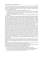
Szarvasi-1 in the course of annual growth (Fig. 18.).

Sustainable Growth and Applications in Renewable Energy Sources

292

Fig. 18. Energy grass field in Baranya county (photo: Róbert W. Pál)
Quantitative analyses of the plant material of Szarvasi-1 were conducted to describe the
chemical profile of the biofuel. Ash and energy content were determined by combustion
experiments in laboratory while the dynamics of firing were studied in different
experimental furnaces. We developed best practices for combusting Szarvasi-1 biofuel.
Dry matter content of Szarvasi-1 is highly influenced by the morphological features of the

vegetative organs. The occurrence and proportion of mechanical and vascular tissues were
investigated in the leaves and culms of Szarvasi-1 in various experimental settings for two
years. Having examined the effect of different soil types on the anatomical characteristics of
the culm and the leaves, we determined the most favourable habitat types of this energy
plant to achieve the highest biomass yields with the greatest dry matter content.
Ecophysiological regulation and the threshold limits of gas exchange parameters
(assimilation, transpiration, water use efficiency, stomatal conductance) of Szarvasi-1
were also investigated. For abiotic environmental variables, air humidity and light had
the most significant effect on gas exchange parameters. Assimilation curves and some
characteristic values (e.g. light compensation and efficiency, assimilation capacity) were
different at the beginning of the growing period on all studied soil types. These
parameters characteristically declined under water-limited environmental conditions.
Water limitation had a slightly positive effect on water use efficiency. Ecophysiological
conclusions, drawn from gas exchange analyses, can be utilized for planning biological
and agronomical aspects to achieve higher biomass production, in accordance with the
abiotic environmental regime.
The typical weed composition and abundance in energy grass fields were compared to other
arable crop cultures. Weed-crop competition was also investigated in different soil
conditions. The weed composition of energy grass fields is more similar to perennial
cultures like alfalfa than to other annual ones (cereals, row crops). Although no herbicide
treatment was carried out, percent cover of Szarvasi-1 energy grass increased significantly
year by year with decreasing weed cover and species number. By the second year, the
average weed cover dropped from the first year’s value of 48 % to 17 % and in the third year
it did not exceed 4 %. Different soil types had different effect on the temporal variation of
weed composition.
Tall Wheatgrass Cultivar Szarvasi–1 (Elymus elongatus subsp. ponticus cv. Szarvasi–1)
as a Potential Energy Crop for Semi-Arid Lands of Eastern Europe

293
In order to maintain a standard quality of Szarvasi-1 as an energy crop, it was essential to

clarify its genetic characteristics. RAPD-based DNA fingerprinting revealed a low level of
genetic variability among samples of the cultivar. In addition, a comparative analysis of
three native Hungarian Elymus elongatus populations and Szarvasi-1 cultivar confirmed their
genetic identity, having found no specific marker characteristic only for the latter. Ecological
risk of unwanted gene exchange among close taxonomic relatives may be rather low but not
impossible according to our results.
Moderate phenotypic plasticity, enormous capability to suppress weeds, high potential to
produce biomass even among drier climatic conditions and a relatively high energy and
moderate ash content suggest that tall wheatgrass cultivar Szarvasi-1 has great potential as a
herbaceous energy plant for arid or semi-arid lands in Eastern Europe.
10. Acknowledgement
Our research and publication were financially supported by NKFP 3A/061/2004 and
TÁMOP-4.2.2/B-10/1-2010-0029. Special thanks should be given to John Michael Lynch and
Emily Rauschert for the thorough linguistic corrections of our manuscript.
11. References
Assadi, M.  Runemark, H. (1995). Hybridization, genomic constitution and generic
delimitation in Elymus sl (Poaceae, Triticeae). Plant Systematics and Evolution Vol.
194, No. 3-4, (September 1995), pp. 189-205, ISSN 0378-2697
Barkworth, M. (2011). Thinopyrum ponticum (Podp.) Z.W. Liu & R.R C. Wang, In:
Thinopyrum Á. Löve, 8 June 2011, Available from:
http:// herbarium.usu.edu/webmanual/info2.asp?name=Thinopyrum_ponticum
Bleby, T.M.; Avcote, M.; Kennett-Smith, A.K.; Walker, G.P. & Schachtman, R.P. (1997).
Seasonal water use characteristics of tall wheatgrass (Agropyron elongatum (Host)
Beauv.) in a saline environment. Plant Cell and Environment Vol. 20, No. 11,
(November 1997), pp. 1361-1371, ISSN 0140-7791
Cox, G.W. (2001). An inventory and analysis of the alien plant flora of New Mexico. The
New Mexico Botanist, Vol. 17, (January 2001), pp. 1-8.
Díaz, O.; Sun, G. L.; Salomon, B. & Bothmer, R. (2000). Levels and distribution of allozyme
and RAPD variation in populations of Elymus fibrosus (Poaceae). Genetic Resource
and Crop Evololution, Vol. 47, No. 1, (February 2000), pp. 11-24, ISSN 0925-9864

Guadagnuolo, R.; Bianchi, D. S. & Felber, F. (2001). Specific genetic markers for wheat, spelt,
and four wild relatives: comparison of isozymes, RAPDs, and wheat
microsatellites. Genome, Vol. 44, No. 4, (July 2001), pp. 610-621, ISSN 0831-2796
Häfliger, E.  Scholz, H. (1980). Grass Weeds. Vol. 2. CIBA-GEIGY Ltd. Basel, Switzerland
Heslop-Harrison, Y.  Shivanna, K.R. (1977). The Receptive Surface of the Angiosperm
Stigma. Annals of Botany Vol. 41, (November 1977), pp. 1233-1258, ISSN 0305-7364
Janowszky, J. & Janowszky, Zs. (2007). A Szarvasi-1 energiafű fajta – egy új növénye a
mezőgazdaságnak és az iparnak (Szarvasi-1 energy grass – a novel crop for the
agriculture and industry) In: Tasi, J. A magyar gyepgazdálkodás 50 éve Gödöllő,
Szt. István Egyetem ISBN 978-963-9483-77-4 pp. 89-92
Johnson, R.C. (1991). Salinity resistance, water relations, and salt content of crested and tall
wheatgrass accessions. Crop Science Vol. 31, (n.d.), pp. 730-734, ISSN 0011-183X

Sustainable Growth and Applications in Renewable Energy Sources

294
Larcher, W. (2003). Physiological Plant Ecology. Ecophysiology and stress physiology of
Functional Groups. Springer-Verlag, ISBN 3-540-43516-6, Berlin Heidelberg New York
Melderis, A. (1980). Elymus L., In: Flora Europaea, Vol. 5. Alismataceae to Orchidaceae
(Monocotyledones), Tutin, T.G.; Heywood, V.H.; Burges, N.A.; Moore, D.M.;
Valentine, D.H.; Walters, S.M.  Webb, D.A., (Eds.), pp. 192-199, Cambridge
University Press, ISBN-13: 9780521153706, Cambridge, England
Mizianty, M.; Frey, L.  Szczepaniak, M. (1999). The Agropyron-Elymus complex (Poaceae)
in Poland: nomenclatural problems. Fragmenta Floristica et Geobotanica Vol. 44,
No. 1, (n.d.), pp. 3-33, ISSN 1640-629X
Molnár, Zs.; Bölöni, J. & Horváth, F. (2008). Threatening factors encountered: Actual
endangerment of the Hungarian (semi-) natural habitats. Acta Botanica Hungarica
Vol. 50(Suppl.), (n.d.), pp. 199-217. ISSN 0236-6495
Murphy, M.A.  Jones, C.E. (1999). Observations on the genus Elymus (Poaceae: Triticeae)
in Australia. Australian Systematic Botany Vol. 12, No. 4 , (n.d.), pp. 593-604, ISSN

1030-1887
Nieto-López, R. M.; Casanova, C. & Soler, C. (2000). Analysis of the genetic diversity of wild,
Spanish populations of the species Elymus caninus (L.) Linnaeus and Elymus
hispanicus (Boiss.) Talavera by PCR-based markers and endosperm proteins.
Agronomie, Vol. 20, No. 8, (December 2000), pp. 893-905 ISSN 0249-5627
Pál R. & Csete S. (2008). Comparative analysis of the weed composition of a new energy crop
(Elymus elongatus subsp. ponticus [Podp.] Melderis cv. Szarvasi-1) in Hungary. Journal
of Plant Diseases and Protection, Vol.21, (March 2008), pp. 215-220, ISSN 1861-4051
Petersen, G. & Seberg, O. (1997). Phylogenetic Analysis of the Triticeae (Poaceae) Based on
rpoA Sequence Data. Molecular Phylogenetics and Evolution, Vol. 7, No. 2, (April
1997), pp. 217-230, ISSN 1055-7903
Podani, J. (1993). SYN-TAX 5.0: Computer programs for multivariate data analysis in
ecology and systematics. Abstracta Botanica, Vol. 17, Part 4 , (n.d.), pp. 289-302,
ISSN 0133-6215
Reisch, C.; Poschlod, P. & Wingender, R. (2003). Genetic differentiation among populations of
Sesleria albicans Kit. ex Schultes (Poaceae) from ecologically different habitats in central
Europe. Heredity, Vol. 91, No. 5, (November 2003), pp. 519-527, ISSN 0018-067X
Salamon-Albert É. & Molnár H. (2009). CO2 gas exchange parameters as the measure of
biomass production of the Hungarian energy grass. Proceedings of International
Symposium on Nutrient Management and Nutrient Demand of Energy Plants July
6-8, 2009 Corvinus University Budapest, Hungary.
Salamon-Albert É. & Molnár H. (2010). Environment regulated ecophysiological responses
of a tall wheatgrass cultivar. Novenytermeles Vol. 59., No. 1., (n.d.), pp. 393-396,
ISSN 2060-8543
Sha, l., Fan, X., Yang, R., Kang, H., Ding, C., Zhang, L., Zheng, Y. & Zhou, Y. (2010). Phylogenetic
relationships between Hystrix and its closely related genera (Triticeae; Poaceae) based
on nuclear Acc1, DMC1 and chloroplast trnL-F sequences. Molecular Phylogenetics and
Evolution, Vol. 54, No. 2, (February 2010), pp. 327-335, ISSN 1055-7903
Swofford, D. L. (2001). PAUP*. Phylogenetic Analysis Using Parsimony (*and Other
Methods) Version 4. Sinauer Associates, Sunderland, Massachusetts

Tutin, T.G.; Heywoog, V.H.; Burges, N.A.; Moore, D.M.; Valentine, D.H.; Walters, S.M. & Webb,
D.A. (1980). Flora Europaea Vol. 5 Alismataceae to Orchidaceae (Monocotyledones),
Cambridge University Press, ISBN 978-052-1201-08-7, Cambridge, UK
Walsh, N.G. (2008). A new species of Poa (Poaceae) from the Victorian Basalt Plain.
Muelleria, Vol. 6, No. 2, (July 2008), pp. 17-20, ISSN 0077-1813
14
Analysis of Time Dependent Valuation of
Emission Factors from the Electricity Sector
C. Gordon and Alan Fung
Ryerson University
Canada
1. Introduction
In recent years, energy consumption and associated Greenhouse Gas (GHG) emissions and
their potential effects on the global climate change have been increasing. Climate change
and global warming has been the subject of intensive investigation provincially, nationally,
and internationally for a number of years. While the complexity of the global climate change
remains difficult to predict, it is important to develop a system to measure the amount of
GHG released into the environment. Thus, the purpose of this chapter is to demonstrate
how several methods can accurately estimate the true GHG emission reduction potential
from renewable technologies and help achieve the goals set out by the Kyoto Protocol -
reducing fuel consumption and related GHG emissions, promoting decentralization of
electricity supply, and encouraging the use of renewable energy technologies.
There are several methods in estimating emission factors from facilities: direct
measurement, mass balance, and engineering estimates. Direct measurement involves
continuous emission monitoring throughout a given period. Mass balance methods involve
the application of conservation equations to a facility, process, or piece of equipment.
Emissions are determined from input/output differences as well as from the accumulation
and depletion of substances. The engineering method involves the use of engineering
principles and knowledge of chemical and physical processes (EnvCan, 2006). In Guler
(2008) the method used to estimate emission factors considers only the total amount of fuel

and electricity produced from power plants. The previous methodology does not take into
consideration the offset cyclical relationship, daily and yearly, between electricity generated
by renewable technologies. It should be noted that none of the methods mentioned above
include seasonal/daily adjustments to annual emission factors. Specifically, the proposed
research would include analyzing existing methods in calculating emission factors and
attempt to estimate new emission factors based on the hourly electricity demand for the
Province of Ontario.
In this Chapter, several GHG emission factor methodology was discussed and compared to
newly developed monthly emission factors in order to realize the true CO
2
reduction
potential for small scale renewable energy technologies. The hourly greenhouse gas
emission factors based on hour-by-hour demand of electricity in Ontario, and the average
Greenhouse Gas Intensity Factor (GHGIF
A
) are estimated by creating a series of emission
factors and their corresponding profiles that can be easily incorporated into simulation

Sustainable Growth and Applications in Renewable Energy Sources

296
software (Gordon & Fung, 2009). The use of regionally specific climate-modeled factors,
such as those identified, allowed for a more accurate representation of the benefits
associated with GHG reducing technologies, such as photovoltaic, wind, etc. This chapter
will demonstrate that using Time Dependent Valuation (TDV) emission factors provide an
upper limit while using hourly emission factors provide a lower limit. These factors based
on hour-by-hour electricity demand data for the Province of Ontario will provide renewable
technology researchers with the tools necessary to make informative decisions concerning
the selection of renewable technologies.
2. Traditional methodologies to estimate GHG emission factors from the

electricity generation sector
There are two main methods to estimate pollutant and GHG emission Factors from the
electricity generation sector: 1) direct measurement or 2) estimation. Direct measurement is
considered to be the most accurate since it uses real-time data from the generation sector.
However, these data are not readily available and historically, GHG emissions have been
estimated from fossil fuel and process-related activities. Estimation is the method used by
several countries when preparing their national GHG inventories (ICPP, 1997). In the past,
GHG emissions from the electricity generation sector were calculated using the Average
GHG Intensity Factor (GHGIF
A
) (Guler et al., 2008). The GHGIF
A
is the amount of GHG
emissions per kWh electricity produced. This method assumes that the reduction in
electricity demand is uniformly distributed amongst all types of electricity generation. For
example, the GHGIF
A
estimated in 1993 was 136 g/kWh for the Province of Ontario. Table 1
shows the GHGIF
A
values for the years 2004, 2005, and 2006 for the Province of Ontario
from the electricity generation sector (EnvCan, 2006).

Annual GHGIF
A
(g of CO
2
/kWh)
2004 2005 2006
200 221 189

Table 1. Annual Emission Factors
The combustion of fossil fuels produces several major greenhouse gases. The amount of
emissions from CO
2
, CH
4
, SO
2
, NO, and N
2
O varies from one fuel to another, and they are
calculated using emission factors. These emission factors are commonly expressed in tons of
CO
2
per MWh or grams per kWh of electricity produced (Gordon & Fung, 2009).
3. Accuracy of GHG emission factors
It is necessary to develop methodology to accurately estimate GHG emissions from the
electricity generation sector in order to facilitate the implementation of awareness
programmes and renewable technologies which are supported with information on current
energy usage. It should be noted that the time of use of electricity is related to GHG
emissions generated throughout the day (MacCracken, 2006). Therefore, prior to
implementing these programmes and renewable technologies, it is necessary to have an
accurate model for emission and electricity estimation.
The Province of Ontario has a very unique mix of electricity production technologies. Hydro
and nuclear technologies are generally considered to be base load power (IESO, 2006), since

Analysis of Time Dependent Valuation of Emission Factors from the Electricity Sector

297
they both operate at constant load and fossil generating plants are typically used to handle

fluctuations in electricity demand throughout the day. The GHGIF
A
estimate is based on the
generation mix for the Province of Ontario (nuclear, hydro, coal, etc.) and is not adequate to
account for most of the GHG emissions from the electricity generation sector, which mainly
come from fossil generating stations. Therefore, in order to estimate and phase out fossil
completely, a different emission factor needs to be developed. In response to this, a second
intensity factor (GHGIF
M
) was developed. The GHGIF
M
intensity factor was calculated by
dividing the net fossil fuel plant electricity production by the total equivalent CO
2

emissions. The value estimated for 1993 was 903.7 t/GWh (Guler et al., 2008). This emission
factor assumes that all electricity consumption is provided by fossil plants. This would be
beneficial if trying to replace all fossil plants with renewable technologies. However, both of
the methodologies neglect to show hourly changes in emission factors.
4. GHG emission factor methodologies
Renewable technologies (solar and wind) have become an accepted form of generating
electricity and heat in the Province of Ontario. There are many advantages in using solar
and wind energy such as taking advantage of an abundant source of free energy (sun and
wind), as well as being an effective method in reducing GHG emissions. However, the
electricity produced by a renewable technology, such as a photovoltaic (PV), or micro-wind
turbine and the availability of solar and wind energy, changes throughout the day.
Therefore, an hourly GHG emission factor is needed to truly understand the impact that
renewable technologies have on emissions since there is a divergence between when
electricity can be generated and when it is required.
Some of these renewable technologies that are being used in the residential and commercial

sectors include photovoltaic, micro-wind turbines, ground source heat pumps, and advance
solar thermal technologies. Continuous improvement of these technolgies have promoted
the development of hybrid homes. The combination of several of these technologies together
will result in end-use energy savings and GHG emission reductions. However, prior to
implementing any of these technologies, it is necessary to have an accurate estimation of the
true reduction potential of GHG emission factors in order to have a clear understanding of
the saving potentials associated with renewable technologies.
Currently, Environment Canada uses fuel consumption data from the electricity sector in
order to estimate emissions. However, this method can be simplistic and time consuming as
well as difficult to use due to the unavailability of certain types of data. Moreover, this
method only provides an annual average emission factor which does not reflect the cyclic
behaviour of emission factors throughout the day. In 2005, Time Dependent Valuation
(TDV) was introduced as a viable method to provide the aformentioned data (MacCracken,
2006). This method was adopted by California as an energy efficient standard for residential
and non-residential buildings. Time dependent valuation views energy demand differently
depending on the time of use (MacCracken, 2006). California has been able to determine the
societal impacts of time of use energy consumption. As a result, this method of analysis
would allow for a more accurate representation of the potential reduction of GHGs by using
renewable technologies.
This following sections will discuss existing emission factor methodolgy and introduce
monthly TDV emission factor methodology.

Sustainable Growth and Applications in Renewable Energy Sources

298
4.1 Hourly GHG emission factors
Different emission factors have been developed in the past: hourly, seasonal, and seasonal
time dependent emission factors (Gordon & Fung, 2009). This chapter will introduce monthly
TDV emission factors and compare them to existing emission factors. GHG emissions from the
electricity generation industry have been calculated using the Average GHG Intensity Factor

(GHGIF
A
) (Guler et al., 2008). This value represents the amount of GHG emissions produced
as a result of generating one kWh of electricity. The GHGIF
A
for 2004, 2005, and 2006 were
estimated using the methodology mentioned above in conjunction with the electricity output
information from Gordon & Fung (2009). It should be noted that the emission factor for CO
2

does not take into consideration CH
4
and N
2
O since these are considered to represent
negligible amounts in comparison to CO
2
, SO
2
, and NO (Gordon & Fung, 2009). This section
will only focus on CO
2
emissions since the majority of pollutants are in this form and the
purpose of this chapter is to demonstrate emission factor methodology.
The GHG emissions due to coal fired and natural gas plants were determined using
Equation 1 (Gordon & Fung, 2009).

2
HCO =(HECOAL)(i)+(HEOTHER)(
j

)
(1)
Where,
HCO
2
= Hourly CO
2
production (kg)
HECOAL = Hourly Electricity generated by Coal plants
HEOTHER = Hourly Electricity generated by Other (natural gas, etc.)
i = CO
2
emission factor (OPG, 2006)
j
= Environment Canada natural gas emission factor (Environment Canada, 2006)
Currently, there is a hourly greenhouse gas emission factor (NHGHGIF
A
) model which is based
on the hour-by-hour demand of electricity in Ontario from nuclear, fossil, hydro, natural gas
and wind (Gordon & Fung, 2009). The NHGHGIF
A
was calculated by dividing the hour-by-
hour emissions from CO
2
by the hour-by-hour total electricity generated from the different
sources (Gordon & Fung, 2009). It should be noted that the new greenhouse gas intensity factor
(NGHGIF
A
) was estimated by taking the average of the hourly emission factors for each season.
The NGHGIF

A
was determined using Equations 2 and 3 (Gordon & Fung, 2009).

2
A
HCO
NHGHGIF
HEGTOTAL

(2)

8760
1
8760
Ai
A
i
NHGHGIF
NGHGIF



(3)
Where,
NHGHGIF
A
= New Hourly Greenhouse Gas Intensity Factor (g
2
CO
/kWh)

NGHGIF
A
= New Greenhouse Gas Intensity Factor (g
2
CO /kWh)
HCO
2
= Hourly CO
2
production (g)
HEGTOTAL= Hourly Electricity Generated Total (kWh)
i = hour
The values obtained for the NGHGIF
A
were compared for the years 2004, 2005, and 2006
(Gordon & Fung, 2009).

Analysis of Time Dependent Valuation of Emission Factors from the Electricity Sector

299
4.2 Seasonal time dependent valuation emission factors
Currently, there are several TDV profiles (annual and seasonal) for greenhouse gases for
the Province of Ontario in the public domain (Gordon & Fung, 2009). As discussed in
Gordon & Fung (2009), the hourly GHG emissions data has been compiled to developed
different types (annual and seasonal) of emission factors. The latter has shown that
emission factors vary with electricity demand (MacCracken, 2006). It has also been
observed that shape and magnitude of GHGIF profiles varies with time of day, year,
climate, and geographical location (Gordon & Fung, 2009). Hourly emission data does
exist from the power generating sector, but is not publicly available. Therefore, rather
than using a single annual GHGIF value for the entire year, seasonal GHGIF profiles

based on the electricity demand for the Province of Ontario were developed by Gordon &
Fung (2009).
The approach detailed below was used in order to provide a better method to properly
estimate greenhouse gases within the Province of Ontario. Hourly electricity consumption
data from the IESO and hourly GHG emission factors estimated in the previous section were
used to determine Seasonal TDV emission factor profiles for the years 2004, 2005, and 2006.
These profiles were calculated using Equation 4 (Gordon & Fung, 2009).

1
N
A
j
i
A
NGHGIF (h )
Seasonal TDV NGHGIF
N



(4)
Where,
Seasonal TDV NGHGIF
A
= Seasonal Time Dependent Valuation New Greenhouse Gas
Intensity Factor (g
2
CO /kWh)
N = number of days in the season
i

= day number
j
= hour number
The hourly and averaged values obtained for the seasonal TDV NGHGIF
A
were compared
for the years 2004, 2005, and 2006.
4.3 Monthly time dependent valuation emission factors
Currently, there are several TDV profiles (annual and seasonal) for greenhouse gases for the
Province of Ontario in the public domain (Gordon & Fung, 2009). However, monthly GHG
emission factors are not available. Therefore, this section will provide renewable technology
professionals with monthly TDV profiles for estimating emissions.
The approach detailed below was used in order to provide a better method to properly
estimate greenhouse gases within the Province of Ontario. Hourly electricity consumption
data from the IESO and hourly GHG emission factors estimated in Section 4.1 were used to
determine monthly TDV NGHGIF profiles for the years 2004, 2005, and 2006. These profiles
were calculated using Equation 5 for each hour in a day.

1
N
A
j
i
A
NGHGIF (h )
Monthly TDV NGHGIF
N




(5)

Sustainable Growth and Applications in Renewable Energy Sources

300
Where,
Monthly TDV NGHGIF
A
= Monthly Time Dependent Valuation New Greenhouse Gas
Intensity Factor (g
2
CO
/kWh)
N = number of days in the month
i = day number
j
= hour number
The hourly and average values obtained for the monthly TDV NGHGIF
A
were compared for
the years 2004, 2005, and 2006.
5. Test case scenario
The following test case provides an example on how the different GHG emission factors can
be used to demonstrate the cyclic behaviour of emission factors througout the day, month,
season, and year. In addtion, the test cases also show the beneficial attributes associated
with renewable technologies.
Transient System Simulation Tool (TRANSYS) building energy simulation software can be
used to perform highly complex thermal analysis, HVAC analysis and electrical power flow
simulations.
Tse et al. (2008) performed simulations, using TRANSYS, which included the use of PV on

the computational model for a townhouse that would be built in the Annex area in Toronto.
TRANSYS was used to simulate and help optimize the performance of the home, as well as
the different systems that would be implemented. The systems that were analyzed consist of
a solar domestic hot water system, a photovoltaic system (6.25 kW), and a ground source
heat pump. Hourly annual simulations were run to demonstrate the potential electricity
contribution and emission savings from PV. This data has been utilized in combination with
the hourly, seasonal and monthly TDV emission factors discussed in the previous sections to
estimate the reduction potential of GHG emissions by the use of PV technology.
6. Results
6.1 Hourly GHG emission factors
The results for the NGHGIF
A
for the years 2004, 2005, and 2006 are shown in Table 2
(Gordon & Fung, 2009).

Season
NGHGIF
A
(g of CO
2
/kWh)
2004 2005 2006
Annual 208 221 189
Winter 248 231 196
Spring 164 205 164
Summer 174 241 214
Fall 244 205 190
Table 2. Hourly annual and seasonal average GHG emission factors
Table 2 shows a large variance between emission factors throughout the year and from year
to year. Clearly, the use of hourly data is necessary to accurately estimate the GHG

reduction potential from renewable technologies.

Analysis of Time Dependent Valuation of Emission Factors from the Electricity Sector

301
6.2 Annual time dependent valuation emission factors
Table A-1 in Appendix A shows the annual TDV emission factors (Gordon & Fung, 2009). It
can be observed that emissions throughout the day vary considerably. It should be noted
that the maximum TDV values for the years 2004, 2005, and 2006 occurred at 1 p.m.
Table 3 shows the annual average TDV GHG emission factors. These values were obtained
by using the annual TDV GHG emission factors in Table A-1 in Appendix A.


NGHGIF
A
(g of CO
2
/kWh)
2004 2005 2006
Annual 224.2 237.3 207.2
Table 3. Annual average TDV GHG emission factors
6.3 Seasonal time dependent valuation emission factors
Seasonal TDV emission factors were also developed for the years 2004, 2005, and 2006 (Gordon
& Fung, 2009) as shown in Table 4. Table A-2 and A-3 in Appendix A show the seasonal TDV
emission factor profiles for 2004, 2005, and 2006. The following can be observed from Table 4:
 For the year 2004 – the highest emission factors were in the fall (afternoons) and winter
(early mornings).


For the years 2005 and 2006 the highest emission factor was observed in the summer.

Season
NGHGIF
A
(g of CO
2
/kWh)
2004 2005 2006
Winter 264.7 246.4 213.4
Spring 182.0 221.5 179.9
Summer 190.1 256.6 229.5
Fall 259.8 224.8 206.1
Table 4. seasonal average TDV GHG emission factors
6.4 Monthly time dependent valuation emission factors
Monthly TDV emission factors were developed for the years 2004, 2005, and 2006 as shown
in Table 5. Table A-4 in Appendix A shows the monthly TDV emission factor profiles for
2004, 2005, and 2006. The following can be observed from Table 4:
 For the year 2004 – the highest and lowest emission factor was observed in January and
May, respectively.


For the year 2005 – the highest and lowest emission factor was observed in August and
May, respectively.


For the year 2005 – the highest and lowest emission factor was observed in July and
April, respectively.

This section discussed the different types of existing and new GHG emission factors for the
years 2004, 2005, and 2006. The hourly emission factor proved to be the most accurate and

monthly TDV were more accurate than using the seasonal average value.
However, it is the user’s responsability to select the appropiate emission factor depending
on the type of analysis conducted. In certain cases it might be more practical to employ
seasonal, time dependent valuation (seasonal or monthly), or annual average emission
factors to estimate CO
2
emissions without sacrificing much accuracy.

Sustainable Growth and Applications in Renewable Energy Sources

302
Season
NGHGIF
A
(g of CO
2
/kWh)
2004 2005 2006
January 284.3 242.2 215.1
February 259.3 228.9 198.8
March 214.5 230.4 180.8
April 171.3 209.6 125.5
May 144.0 183.2 164.8
June 156.0 238.7 216.9
July 166.4 236.8 233.9
August 179.4 245.4 205.3
September 210.9 222.1 188.0
October 265.0 206.0 193.6
November 242.4 192.9 191.1
December 199.9 214.3 155.4

Table 5. Monthly TDV average GHG emission factors
6.5 Test case study
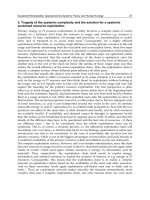
The electricity generated by the PV simulations performed for 2005 is illustrated in Figure 1
(Tse et al., 2008). It can be observed that PV electricity generation was the highest during the
summer.
Table 6 shows the total electric power generated by PV for year 2005 using the test case
townhouse located in the Annex part of Toronto (Tse et al., 2008).

Photovoltaic
Electricity Generated (kWh)
7767
Table 6. Total electricity generated by PV for test case study
Figure 1 shows the total monthly electric power generated by the PV system for the year
2005. Electricity generation was the highest during July and throughout the summer.

Analysis of Time Dependent Valuation of Emission Factors from the Electricity Sector

303
0
200
400
600
800
1000
1200
Jan Feb Mar Apr May Jun Jul Aug Sep Oct Nov Dec
Electricity Generated (kWh)
PV

Fig. 1. Monthly electricity generated by PV for test-case study

In order to calculate the CO
2
emission reduction potential by PV, the hourly electricity data
was multiplied by the different emission factors as defined in Equations 6, 7, 8, 9 (Gordon &
Fung, 2009), and 10.

A
el,HNGHGIF
GHG





el,hourly A
Generated NHGHGIF






(6)
Where,
A
el,HNGHGIF
GHG

Annual GHG emission reduction using the new hourly emission factor
(g of CO

2
)
el,hourl
y
Generated = Hourly electricity generated by renewable technology for test case
house (kWh)
A
NHGHGIF = New Hourly Greenhouse Gas Intensity Factor (g CO
2
/kWh)

A
el,SANGHGIF
GHG
=




el,hourly A
Generated SANGHGIF





(7)
Where,
A
el,SANGHGIF

GHG = Annual GHG emission reductions using the seasonal average emission
factor (g of CO
2
)
el,hourl
y
Generated = Hourly electricity generated by renewable technology for test case
house (kWh)
A
SANGHGIF = Seasonal Average New Greenhouse Gas Intensity Factor (g CO
2
/kWh)

A
el,AANGHGIF
GHG =



el,hourly A
Generated AANGHGIF





(8)

Sustainable Growth and Applications in Renewable Energy Sources

304
Where,
A
el,AANGHGIF
GHG = Annual GHG emission reductions using the annual average emission
factor (g of CO
2
)
el,hourl
y
Generated = Hourly electricity generated by renewable technology for test case
house (kWh)
A
AANGHGIF = Annual Average New Greenhouse Gas Intensity Factor (g CO
2
/kWh)

A
el,TDVNGHGIF
GHG =



el,hourly A
Generated TDVNGHGIF






(9)
Where,
A
el,TDVNGHGIF
GHG = Annual GHG emission reductions using the seasonal time dependent
valuation new greenhouse gas intensity factor (g CO
2
/kWh)
el,hourl
y
Generated = Hourly electricity generated by renewable technology for test case
house (kWh)
A
TDVNGHGIF = Seasonal Time Dependent Valuation New Greenhouse Gas Intensity
Factor (g CO
2
/kWh)

A
el,TDVNGHGIF
GHG =



el,hourly A
Generated TDVNGHGIF






(10)
Where,
A
el,TDVNGHGIF
GHG = Annual GHG emission reductions using the monthly time dependent
valuation new greenhouse gas intensity factor (g CO
2
/kWh)
el,hourl
y
Generated = Hourly electricity generated by renewable technology for test case
house (kWh)
A
TDVNGHGIF = Monthly Time Dependent Valuation New Greenhouse Gas Intensity
Factor (g CO
2
/kWh)
Table 7 summarizes the total emission reduction results from PV by using the different
emission factors. The upper and lower limits of CO
2
reductions were obtained by using the
seasonal TDV and annual average emission factors, respectively. It should be noted that the
new monthly TDV emission factors resulted in an emission reduction potential very close to
that of using hourly emission factors.

Emission Factor Type
Emission Reduction
Potential (kg of CO
2

)
% Difference
Hourly 1856
Seasonal Average 1727 -6.97
Annual Average 1716 -7.54
Seasonal TDV 1974 6.36
Monthly TDV 1854 -0.12
Table 7. Emission reduction potential comparison for test case study

Analysis of Time Dependent Valuation of Emission Factors from the Electricity Sector

305
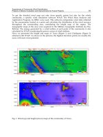
The total monthly emission reduction potential by PV is shown in Figure 2. During June and
July the emission reductions were the highest and in November, the lowest.



0
50
100
150
200
250
300
Jan Feb Mar Apr May Jun Jul Aug Sep Oct Nov Dec
Emission Reductions (kg of CO
2
)

Fig. 2. Monthly emission reductions for PV test case study
7. Conclusion
Several emission factors were developed for the years 2004, 2005, and 2006. The hourly
emission factor proved to be the most accurate. In addition, depending on the type of
analysis conducted it might be practical but not as accurate to employ seasonal, time
dependent valuation, or annual averages emission factors to estimate CO
2
emissions. It was
observed that TDV and seasonal average emission factors were more accurate than using
the annual average value. It should also be mentioned, that monthly TDV emission factors
proved to be as accurate as using hourly values. The use of hourly emission factors to
accurately estimate the potential reduction of renewable technologies should be
incorporated in all renewable technology assesments.
8. Recommendations
This chapter discussed the use of hourly, seasonal, monthly and annual emission factors in
order to demonstrate the daily fluctuations from the electricity generation sector. In the
future, peak, weekly and marginal emission factors could be developed in order to increase
the accuracy of emission estimations. In addition, emission factors could be updated every
year in order to allign with current renewable technology analysis models and electricity
generation mix.

Sustainable Growth and Applications in Renewable Energy Sources

306
9. Appendix A
Annual
TDV NGHGIF
A

(g of CO2/kWh)
Hour 2004 2005 2006
1
185.9 219.7 181.2
2 179.2 213.3 170.5
3 173.6 206.2 161.5
4
171.6 203.9 159.4
5 177.1 209.1 167.9
6 192.5 216.8 178.3
7 210.7 223.7 191.5
8
227.8 236.7 209.1
9 237.0 244.2 218.3
10 243.6 248.5 223.1
11
248.1 251.5 227.3
12 251.1 253.6 229.5
13 253.0 255.6 229.9
14 252.0 255.2 228.7
15 249.7 252.9 225.4
16 248.4 249.3 223.3
17 247.8 248.3 223.7
18 246.5 249.6 224.9
19 244.3 248.6 225.5
20 246.6 249.0 228.1
21 246.9 252.1 228.0
22 236.4 247.3 219.5
23 215.2 235.0 207.0
24 195.0 226.0 191.4

Table A-1. Annual TDV emission factor comparison for 2004-2006

Analysis of Time Dependent Valuation of Emission Factors from the Electricity Sector

307
Winter Spring
TDV NGHGIF
A
(g of CO2/kWh) TDV NGHGIF
A
(g of CO2/kWh)
Hour 2004 2005 2006 Hour 2004 2005 2006
1
254.9 241.8 200.7
1
133.3 192.3 147.0
2
254.8 234.8 191.4
2
129.1 188.5 138.9
3
252.9 229.3 183.1
3
126.6 180.0 132.9
4
250.9 226.8 179.8
4
125.6 179.0 130.8
5
252.4 227.5 183.8

5
130.7 186.8 140.2
6
255.3 231.9 186.5
6
148.2 201.2 153.0
7
258.8 234.7 196.6
7
171.0 213.2 171.3
8
262.5 240.9 208.5
8
192.4 228.5 189.7
9
265.6 247.1 216.3
9
203.0 234.2 194.5
10
266.8 250.5 219.7
10
208.7 237.0 198.7
11
268.8 253.1 225.7
11
213.2 239.8 202.8
12
270.9 254.8 228.5
12
214.8 241.8 204.5

13
272.8 256.5 229.0
13
215.5 244.3 204.4
14
272.8 256.5 227.8
14
215.2 244.1 203.4
15
271.3 252.8 224.8
15
212.3 242.0 201.3
16
268.8 246.5 219.2
16
212.4 240.8 200.7
17
268.6 244.9 218.8
17
212.4 240.5 201.1
18
270.9 250.3 224.4
18
205.0 234.4 195.9
19
274.6 257.5 233.3
19
198.5 224.8 190.5
20
273.4 258.5 235.3

20
204.2 228.6 198.7
21
273.3 260.1 234.2
21
206.5 238.3 203.1
22
271.4 259.2 229.1
22
190.3 231.9 187.3
23
265.4 253.5 217.6
23
161.5 218.2 170.4
24
255.3 243.3 207.8
24
138.8 206.0 155.6
Table A-2. Seasonal TDV GHG Emission Factors for Winter and Spring

Sustainable Growth and Applications in Renewable Energy Sources

308
Summer Fall
TDV NGHGIFA (g of CO2/kWh) TDV NGHGIFA (g of CO2/kWh)
Hour 2004 2005 2006 Hour 2004 2005 2006
1
129.4 244.9 199.8
1
226.1 199.9 177.2

2
119.8 236.6 186.5
2
213.2 193.4 165.1
3
112.5 227.6 175.2
3
202.5 187.9 154.8
4
109.9 224.1 173.2
4
200.2 185.7 153.8
5
114.3 225.6 181.9
5
210.9 196.5 165.8
6
134.7 229.1 189.5
6
231.7 205.0 184.0
7
159.5 232.4 202.1
7
253.4 214.3 196.0
8
187.5 251.1 227.3
8
268.7 226.4 211.0
9
205.0 262.4 243.1

9
274.5 233.2 219.4
10
220.1 268.1 250.7
10
278.8 238.4 223.4
11
228.3 270.4 254.0
11
282.2 242.6 226.6
12
234.5 273.4 256.3
12
284.2 244.4 228.5
13
237.8 276.7 256.3
13
285.7 245.0 230.0
14
236.6 276.4 254.6
14
283.5 243.8 229.1
15
234.1 275.3 251.0
15
281.3 241.3 224.5
16
234.7 273.5 251.3
16
277.4 236.3 221.8

17
234.4 272.4 252.9
17
275.9 235.4 221.8
18
228.5 272.1 252.0
18
281.7 241.4 227.3
19
218.7 267.5 248.3
19
285.5 244.4 229.8
20
223.3 267.3 251.3
20
285.4 241.8 227.1
21
226.3 269.8 252.6
21
281.5 240.2 222.2
22
209.7 264.3 245.7
22
274.0 233.9 216.1
23
176.2 249.8 236.9
23
257.9 218.4 202.9
24
146.7 248.7 214.9

24
239.2 206.1 187.5
Table A-3. Seasonal TDV GHG Emission Factors for Summer and Fall

Analysis of Time Dependent Valuation of Emission Factors from the Electricity Sector

309
J
anuar
y

Februar
y

TDV NGHGIF
A

(
g
of CO2/kWh)

TDV NGHGIF
A

(
g
of CO2/kWh)
Hour 2004

2005

2006

Hour

2004

2005

2006
1
282.1

229.9

195.4

1

254.4

221.2

183.0
2
288.0

226.7

184.4

2

251.0

210.6

174.1
3 286.6

224.6

174.3

3

248.6

203.0

168.0
4 285.0

221.4

169.0

4

245.2

201.2

165.5
5 283.9

221.2

172.5

5

252.0

203.9

169.8
6 283.1

222.6

177.0

6

256.5

212.1

173.6

7 279.3

223.0

190.0

7

258.5

220.0

184.0
8 278.0

231.9

210.2

8

260.3

228.9

196.5
9 280.2

241.9

221.7

9

263.7

234.0

203.7
10 280.1

244.0

222.7

10

264.0

236.1

207.3
11
280.5

248.4

228.0

11

264.7

238.4

214.9
12
282.2

251.1

232.1

12

264.6

238.5

216.3
13 285.4

253.7

233.7

13

266.6

241.0

215.2
14 286.5

256.6

235.2

14

268.1

239.9

213.4
15 287.0

251.7

233.9

15

265.6

236.0

209.5
16 285.8

246.0

224.5

16

260.5

230.3

206.3
17 283.3

245.4

224.5

17

258.3

228.4

205.0
18 284.5

251.8

233.5

18

257.9

231.6

205.4
19 289.6

258.7

244.5

19

262.6

240.9

219.0
20 287.5

257.2

241.6

20

264.6

246.0

223.2
21
287.9

258.7

240.7

21

265.2

246.5

220.7
22
287.7

256.9

236.7

22

264.2

244.6

213.9
23 286.4

249.9

227.9

23

257.5

238.6

195.6
24 281.4

238.9

208.7

24

248.1

222.3

187.1
March

A
p
ril

TDV NGHGIF
A

(
g
of CO2/kWh)

TDV NGHGIF
A

(
g
of CO2/kWh)
Hour 2004

2005

2006

Hour

2004

2005

2006

1 191.2

228.4

172.8

1

116.9

177.5

79.7
2
189.0

223.7

164.0

2

115.1

175.7

74.9
3
187.4

217.9

153.9

3

114.6

167.2

73.7
4 185.6

215.7

150.9

4

115.6

167.9

76.1
5 184.9

218.5

155.3

5

124.2

176.9

82.3
6 192.3

225.1

158.6

6

147.0

197.9

99.0
7 205.3

227.6

170.8

7

168.2

207.5

121.3
8 218.1

227.8

179.1

8

188.0

219.8

138.7
9 224.8

233.2

185.2

9

196.1

224.8

144.1
10 225.1

235.3

188.7

10

201.3

229.1

151.5
11 227.2

236.3

192.2

11

204.2

230.6

155.4
12
230.4

239.7

193.6

12

204.1

230.7

157.4
13
230.2

241.5

194.1

13

204.5

232.4

155.7
14 231.8

240.3

193.4

14

203.8

230.9

153.3
15 229.0

237.5

193.2

15

201.8

229.9

149.3
16 228.5

233.3

189.2

16

199.9

231.1

148.0
17 228.2

231.5

187.9

17

197.9

229.9

146.4
18 225.8

229.9

185.2

18

189.2

221.8

139.5
19 225.4

226.2

183.8

19

183.2

211.1

134.5
20 228.9

229.9

196.4

20

196.0

219.0

150.9
21 229.1

232.8

198.1

21

198.1

227.1

155.8
22
223.2

235.2

193.4

22

176.1

213.8

129.5
23
210.3

232.1

182.6

23

145.9

197.9

105.1
24 195.7

230.3

176.9

24

120.4

180.0

89.4
Table A-4. Monthly TDV GHG Emission Factors for the years 2004, 2005, and 2006

Sustainable Growth and Applications in Renewable Energy Sources

310
Ma
y

J
une

TDV NGHGIF

A

(
g
of CO2/kWh)

TDV NGHGIF
A

(
g
of CO2/kWh)
Hour 2004

2005

2006

Hour

2004

2005

2006
1
87.4

147.5

129.1

1

106.4

215.9

194.7
2
80.3

143.0

123.9

2

102.3

208.1

181.1
3 78.8

134.0

117.5

3

94.5

197.4

169.5
4 78.1

135.9

115.5

4

91.3

191.1

161.9
5 83.8

146.6

130.6

5

93.5

194.7

168.9
6 101.9

163.8

142.3

6

110.6

199.7

180.1
7 132.0

175.9

158.1

7

134.9

216.6

201.0
8 156.6

192.7

176.8

8

158.2

241.7

223.1
9 168.1

197.1

180.4

9

173.1

251.5

227.5
10 175.3

199.1

181.8

10

184.3

254.4

231.6
11
180.8

202.9

185.2

11

190.5

257.7

235.8
12
180.9

206.4

187.3

12

196.1

259.4

238.7
13 182.1

209.0

188.0

13

198.2

261.1

239.0
14 181.4

209.4

186.4

14

196.9

259.9

238.7
15 178.7

208.2

184.2

15

193.6

257.3

237.1
16 180.7

204.4

184.5

16

194.3

256.6

239.2
17 180.8

203.6

187.1

17

193.9

256.6

241.7
18 172.8

194.8

182.7

18

184.6

255.1

236.1
19 164.8

185.5

178.2

19

175.6

250.0

230.5
20 168.1

187.8

183.1

20

174.7

251.1

232.1
21
170.5

201.4

186.0

21

177.6

259.1

236.3
22
152.0

196.7

171.9

22

169.5

256.3

230.5
23 120.8

181.8

154.6

23

137.7

241.7

224.1

24 99.5

169.5

140.5

24

112.9

236.3

206.5
J
ul
y

Au
g
ust

TDV NGHGIF
A

(
g
of CO2/kWh)

TDV NGHGIF
A

(
g
of CO2/kWh)
Hour 2004

2005

2006

Hour

2004

2005

2006
1 108.1

227.5

213.4

1

123.7

236.7

174.9

2
98.2

216.4

200.6

2

113.7

230.3

158.5
3
92.8

207.3

188.6

3

106.1

220.2

146.9
4 91.4

203.8

183.7

4

101.6

217.2

145.7
5 96.7

203.2

187.5

5

103.7

219.0

156.9
6 111.3

202.4

186.1

6

125.3

221.8

163.9
7 131.4

204.0

197.0

7

146.6

221.5

173.8
8 157.4

228.6

225.1

8

177.9

239.2

201.5
9 175.8

244.3

243.1

9

195.5

247.5

218.4
10 191.4

251.0

252.4

10

209.2

253.8

227.6
11 201.6

251.0

257.0

11

216.3

257.3

230.3
12
207.4

251.8

260.0

12

223.2

260.5

232.7
13
212.0

255.7

260.3

13

226.9

264.1

233.5
14 210.6

257.2

258.8

14

225.4

264.1

233.3
15 209.1

256.2

255.6

15

221.9

262.0

229.2
16 209.0

255.5

252.3

16

220.4

260.7

230.7
17 210.3

255.5

252.5

17

218.8

259.2

233.2
18 205.7

254.5

253.6

18

212.3

260.5

232.2
19 196.0

251.2

250.3

19

201.2

255.7

228.8
20 194.1

246.3

249.4

20

208.6

254.6

228.7
21 199.4

248.3

253.0

21

219.5

261.2

232.5
22
193.5

248.7

252.8

22

201.8

251.8

220.6
23
159.8

235.0

248.2

23

167.3

232.4

209.7
24 130.3

228.5

232.4

24

139.1

238.0

184.5
Table A-4. (Continued)