Báo cáo hóa học: " Kinematic variability, fractal dynamics and local dynamic stability of treadmill walking" ppt

JNER
JOURNAL OF NEUROENGINEERING
AND REHABILITATION
Kinematic variability, fractal dynamics and local
dynamic stability of treadmill walking
Terrier and Dériaz
Terrier and Dériaz Journal of NeuroEngineering and Rehabilitation 2011, 8:12
(24 February 2011)
RESEARCH Open Access
Kinematic variability, fractal dynamics and local
dynamic stability of treadmill walking
Philippe Terrier
1,2*
, Olivier Dériaz
1,2
Abstract
Background: Motorized treadmills are widely used in research or in clinical therapy. Small kinematics, kinetic s and
energetics changes induced by Treadmill Walking (TW) as compared to Overground Walking (OW) have been
reported in literature. The purpose of the present study was to characterize the differences between OW and TW
in terms of stride-to-stride variability. Classical (Standard Deviation, SD) and non-linear (fractal dynamics, local
dynamic stability) methods were used. In addition, the correlations between the different variability indexes were
analyzed.
Methods: Twenty healthy subjects performed 10 min TW and OW in a random sequence. A triaxial accelerometer
recorded trunk accelerations. Kinematic variability was computed as the average SD (MeanSD) of acceleration
patterns amo ng standardized strides. Fractal dynamics (scaling exponent a) was assessed by Detrended Fluctuation
Analysis (DFA) of stride intervals. Short-term and long-term dynamic stability were estimated by computing the
maximal Lyapunov exponents of acceleration signals.
Results: TW did not modify kinematic gait variability as compared to OW (multivariate T
2
, p = 0.87). Conversely,
TW significantly modified fractal dynamics (t-test, p = 0.01), and both short and long term local dynamic stability

(T
2
p = 0.0002). No relationship was observed between variability indexes with the exception of significant
negative correlation between MeanSD and dynamic stability in TW (3 × 6 canonical correlation, r = 0.94).
Conclusions: Treadmill induced a less correlated pattern in the stride intervals and increased gait stability, but did
not modify kinematic variability in healthy subjects. This could be due to changes in perceptual information
induced by treadmill walking that would affect locomotor control of the gait and hence specifically alter non-linear
dependencies among consecutive strides. Consequently, the type of walking (i.e. treadmill or overground) is
important to consider in each protocol design.
Introduction
Walking is a repetitive movement which is characterized
by a low variability [1]. This motor skill requires not
only conscious neuromotor tasks but also complex auto-
mated regulation, both interacting to produce steady
gait pattern. Classically, gait variabili ty (i.a. kinematic
variability) has been assessed from the differences
among the strides (Standard Deviation SD, coefficient of
variation CV), i.e. each stride considered as an indepen-
dent event resulting from a random process. However,
this approach fails to account for the presence of feed-
back loops in the motor control of walking: the walking
pattern at a given gait cycle may have consequences on
subsequent strides. As a result, correlations between
consecutive gait cycles and non-l inear dependencies are
expected.
During the last decades, various new mathematical
tools have been used to better characterise the non-
linear features of gait variability. With the Detrended
Fluctuation Analysis (DFA [2-4]) it has be en observed
that the stride interval (i.e. time to complete a gait

cycle) at any time was related (in a statistical sense) to
intervals at relatively remote times (persistent pattern
over more than 100 strides). This dependence (memory
effect) decayed in a power-law fashion, similar to scale-
free, fractal-like phenomena (fractal dynamics [1,3-5]),
also known as 1/f
b
noise [6]).
Another non-linear approach was proposed to charac-
terize the dynamic variability in continuous walking.
* Correspondence:
1
IRR, Institut de Recherche en Réadaptation, Sion, Switzerland
Full list of author information is available at the end of the article
Terrier and Dériaz Journal of NeuroEngineering and Rehabilitation 2011, 8:12
/>JNER
JOURNAL OF NEUROENGINEERING
AND REHABILITATION
© 2011 Terrier and Dériaz; licensee BioMed Central Ltd. This is an Open Access article distributed under the terms of the Creative
Commons Attribution License ( whic h permits unrestricted use, distribution, and
reproduction in any medium, provided the original work is properly cited.
The sensitivity of a dynamical system to small perturba-
tions can be quantified by the system maximal Lyapu-
nov exponent, which characterizes the average rate of
divergence in pseudo-periodic processes [7]. This
method allows to evaluate the ability of locomotor sys-
tem to maintain continuous motion by accommodating
infinitesimally small perturbations that occur naturally
during walking [8]. This includes external perturbations
induced by small variations in the walking surface, as

well as internal perturbations resulting from the natural
noise present in the neuromuscular system [8].
Many theoretical questions are still open about the
validity and application of these methods. For instance,
DFA results are difficult to interpret [9], and no defini-
tive conclusion on the presence of long range correla-
tions should be drawn relying only on it. In addition,
the underlying mechanism of long range correlations in
stride interval is not fully understo od [3,10]. West &
Latka suggested that the observed s caling in inter-stride
interval data may not be due to long-term memory
alone, but may, in fact, be due p artly to the statistics
[11]. It was also suggested that the use of m ulti-fractal
spectrum could be a better approach than mono-fractal
analysis, such as DFA [12,13]. There are also several
methodological issues to compute consistent and reli-
able stability index [14,15].
In parallel with the ongoing theoretical research on
non-linear analysis of physiological time series, the use
of non-linear bio-markers in applied clinical research
has been already fruitful. In the field of human locomo-
tion, it has been demonstrated that gait variability could
serve as a sensitive and clinically relevant tool in the
evaluation of mobility and the response to therapeutic
interventions. For in stance, gait variability (SD and
dynamics) is altered in clinically relevant syndromes,
such as falling and neuro-degenerative disease [16,17].
Gait instability measurement apparently predict falls in
idiopathic elderly fallers [18]. Improvements in muscle
function are associated with e nhanced gait stability in

elderly [19].
Motorized treadmills are widely used in biomechanical
studies of human locomotion. They allow the documen-
tation of a large number of successive strides under con-
trolled enviro nment, with a selectable steady-state
locomotion speed. In the rehabilitat ion field, treadmill
walking is used in locomotor therapy, for instance with
partial body weight support in spinal cord injury or
stroke rehabilitation [20,21]. Since the classical work of
Van Ingen Schenau [22], it is admitt ed that overground
and treadmill locomotion are similar if treadmill belt
speed is constant. Nevertheless, both walking types pre-
sent small differences in kinematics [23,24], kinetics [25]
and energetics [26]. It was also ob served that treadmill
locomotion induced shorter step lengths and higher
cadences than walking on the floor at the same speed
[26,27]. There is still a matter of debate to interpret
such subtle differences [28,29].
It is obvious that treadmill walking (TW) induces spe-
cific kinaesthetic and perceptual information. Previous
studies confirmed that vision plays a central role in the
control of locomotion [30,31]. These differences in
visual afferences b etween TW and Overground Walking
(OW) may induce a modification in motor c ontrol, and
consequently in gait variability.
In 2000, D ingwell et al. anal yzed TW l ocal dynamic
stability (maximal Lyapunov exponent) in 10 healthy
subjects [8,32]. T hey highlighted significant differences
between TW and OW by evaluating local dynamic sta-
bility of lower limbs kinematics [8]. The effect was low

in upper body accelerations. Later [32], they calculated
more specifically short term stability and found a strong
effect of TW in trunk accelerations. On the other hand,
they found a greater kinematic variability at the lower
limb level in OW as compared to TW, but no signifi-
cant difference in trunk kinematics.
In 2005, Terrier et al. [1], by using high accuracy GPS,
described low stride-to-stride variability of speed, step
length and step duration in free walking. They observed
that the constraint of rhythmical auditory signal
("metronome walking”) did not alter kinematic variabil-
ity, but modify the fractal dynamics (DFA) of the stride
interval (anti-persistent pattern).
Based on these previous works, the working hypoth-
esis of the present article is 1) that the constraint of
TW (constant speed, narrow pathway) may induce a less
persistent pattern in the stride int erval, by analogy to
theconstraintinducedbyametronome;2)thatTW
may increase the local dynamic stability of walking, due
to the diminution of degrees of freedom in the more
constrained artificial e nvironment [32,33], 3) that, for
the same reasons, TW may slightly reduce kinematic
variability [32,33] 4) that no correlation exist between
the 3 variability indexes, because they are related to dif-
ferent aspects of the locomotion process.
The purpose of the present study was to analyze, by
using trunk accelerometry, differences between TW and
OW in terms of stride-to-stride kinematic variability
(SD), fractal dynamics (by D FA) and local dynamic s ta-
bility (maximal Lyapunov exponent). In addition, we

ass essed the strength of the r elationships between these
variables (canonical correlation analysis).
Methods
Participants
Twenty healthy male subjects, with no neurological defi-
cit or orthopaedic imp airment, participated to the study.
Most of them were recruited among participants of a
previous “treadmill” study implying only males subjects
Terrier and Dériaz Journal of NeuroEngineering and Rehabilitation 2011, 8:12
/>Page 2 of 13
[34]. Their characteristics were (mean ± SD): age 35 ±
7 yr, body mass 79 ± 10 kg, and height 1.8 0 ± 0.06 m.
All subjects were well trained to walk on a treadmill
before the beginning of the study. The experimental
protocol was approved by the lo cal ethics committee
(commission d’éthique du Valais).
Apparatus
The motion sensor (Physilog system, BioAGM, Switzerland
[35]) was a triaxial accelerometer connected to a data log-
ger recording body accelerations in medio-lateral (ML),
vertical (V) and ante ro-posterior (AP) dire ctions. The
dimensions of the logger were 130 × 68 × 30 mm and the
weight was 285 g. The accelerometers are piezoresistive
sensors coupled with amplif iers (± 5 g, 500 mV/g) and
mounted on a belt. The signals were sampled at 200 Hz
with 12-bit resolution. After each experiment, the data
were downloaded to a PC c omputer and converted in
earth acceleration units (g) according to a previous calibra-
tion. Data analysis was then performed by using Matlab
(Mathworks, Natick MA, USA) and Stata 11.0 (StataCorp

LP, TX, USA)
Procedures
The subjects performed 10 min. treadmill walking (TW)
and 10 min. overground walking (OW) in a random
order. A rest period of five minutes (sitting stil l) was
imposed between the two trials. The motor-driven
treadmill was a Technogym, (Runrace, Italy). The
imposed speed was 1.25 m/s (4.5 km/h) for all subjects:
in the context of a previous study [34], we assessed
average running and walking preferred speed on the
same treadmill in 88 male subjects; an average of 1.26 ±
0.13 m/s was ob served. A thirty second w arm-up was
performed before the beginning of the measurement.
For the OW test, the subjects walked along a standar-
dized 800 m indoor circuit along hospital corridors and
halls. The circuit exhibited only 90° turns. A l arge part
(about 400 m) of the circuit was constituted by a long
corridor. Other people working in the hospital were pre-
sent in the halls. Hence, the OW trials mimicked actual
condition of walking. Subects were asked to walk at
their Preferred Walking Speed (PWS) with a regular
pace. Under both conditions, the accelerometer was
attached to the low back (L4-L5 region) with an elastic
belt, and the logger was worn on the side of the body.
Subjects wore their own low-rise comfortable walking
shoes.
Stride intervals and kinematic variability
Five se conds were removed at the beginning and at the
end of the 10 min. acceleration measurements in order
to avoid non-stationary periods. Heel strike was detected

in the raw acceleration AP signal with a peak de tection
method designed to minimize the risk of false st ep
detection: first, we generated a low-pass filtered version
of the signal (4 o rder Butterwo rth, 3 Hz, zero-p hase fil-
tering). The time of each local minimum was detected.
By superimposing the Filtered Signal (FS) to the original,
Unfiltered Signal (US), we tracked the nearest peak in
US of each local minimum in FS. US peak time was
then chosen as the limit between two steps (Figu re 1A).
The strides were defined as two consecutive steps. On
average, the number of strides was 543 per trial.
Time series of the stride intervals were used to com-
pute a traditional variability index (Coefficient of Varia-
tion of the stride time, CV = SD/Mean*100, Figure 1B).
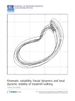
Moreover, the variability of the acceleration pattern
among strides was evaluated as follows (Figure 2): each
stride was normalized to 200 sample points by using a
polyphase filter implementation (Matlab command
Resample); the average stride-to-stride Standard Devia-
tion across all data points ((SD(i) ∀ i Î [1 200])) was
evaluated (MeanSD = 〈SD(i)〉).
Detrended Fluctuation Analysis
The presence of long range correlati ons in the time ser-
ies of stride intervals (fractal dynamics) was assessed by
the use of the non-linear DFA method. Strictly speaking,
0 1 2
−0.5
0
0.5
A

Peak detection
Acce
l
.
(
g
)
Time (s)
0 100 200 300 400 500
1.05
1.1
1.15
1.2
B
Mean=1.1s
CV=1.6%
Time series of stride intervals
#

st
ri
de
Stride time (s)
10
1
10
2
10
−2
10

−1
n
F(n)
DFA: F(n) ~ n
α
with α = 0.84
C
filtred raw
stride #1
stride #2
Figure 1 Method: Step detection, st ride intervals and
Detrended Fluctuation Analysis. One subject performed 10 min
of free walking. A: 2.5s sample of the antero-posterior acceleration
signal; red dotted line is a low pass filtered (<3 Hz) version of the
raw signal (black continuous line). Cross and black circle indicate
how the algorithm specifically detect the heel strike (see method
section for further explanation). The duration of two consecutive
steps is defined as stride interval. B: Time series of stride intervals
during the 10 min walking test. Average stride time (mean) and CV
(SD/mean * 100) is also presented. C: Detredend Fluctuation
Analysis (DFA). The fractal dynamics of the time series (B) is
characterized by the scaling exponent a, computed by comparing
the fluctuation (F(n)) at different scales (n) in a log-log plot.
Terrier and Dériaz Journal of NeuroEngineering and Rehabilitation 2011, 8:12
/>Page 3 of 13
this non-linear method should be used in addition to
other statistical tools to definitivel y conclude that a pro-
cess is a true 1/f
b
noise with power-law decrease of long

range auto-correlations [6,9]. However, DFA has been
successfully used as relevant biomarker in numerous
studies [ 1,16,17,36,37]. Detrended Fluctuation Analysis
is based on a classic root-mean square analysis of a ran-
dom walk, but is specifically designed to be less likely
affected by nonstationarities. Full details of the metho-
dology are published elsewhere [1-4]. In short, the inte-
grated time series of length N is divided into boxes of
equal length, n. In each box of length n, a least squares
line is fit to the data (representing the trend in that
box). The y coordinate of the straight line segments is
denoted by y
n
(k). Next, the integrated time series, y(k),
was detrended, by subtracting the local trend, y
n
(k), in
each box. The root-mean-square fluctuation of this inte-
grated and detrended time series is calculated by
Fn
N
yk y k
n
k
N
() [() ()]=−
=
∑
1
2

1
(1)
This computation is repeated over all box sizes (from
4 to 200) to characterize the relationship between F(n),
the average fluctuation, and the box size, n. The fluctua-
tions can be characterized by the scaling exponent a,
which is the slope o f the line relating log F(n)tolog(n)
(F(n) ~ n
a
), Figure 1C). Long range correlations are pre-
sentintheoriginaltimeserieswhena lies between 0.5
and 1 [3,4].
In a finite length time series, an uncorrelated process
could exhibit “by chance” a scaling exponent different
from the theoretical 0.5 value. To statistically differenti-
ate the stride time series from a random uncorrelated
process, we applied the surrogate data method [1,3]. This
method increases the confi dence that the analyzed series
exhibits long-range correlation. Twenty different surro-
gate data sets were generated by shuffling the original
time series in a random order. On each data set, DFA
analysis was performed to calculate a value. The standard
deviation and mean of this sample was calculated and
compared to a exponent of the original series. The result
is considered significant if the original a is 2 s tandard
deviation away from the mean of the surrogate data set.
Local dynamic stability
The method for quantifying the local dynamical st ability
of the gait by using largest Lyapunov exponent has been
extensively described in literature [ 8]. It examines struc-

tural characteristics of a time series th at is embedded in
an appropriately constructed state space. A valid state
space contains a sufficient number of independent coor-
dinates to define the state of the system unequivocally
[38]. According to the Takens’ theorem, an appropriate
state space can be reconstructed from a single time ser-
ies using the original data and its time delayed copies
(figure 3A) [38].
Xt xt xt T xt T xt d T
E
( ) [ ( ), ( ), ( ), , ( ( ) ]=++ +−21
(2)
Where X(t) is the d
E
-dimensional state vector, x(t) are
the original data, T is the time delay, and d
E
is the
−0.4
−0.2
0
0.2
0.4
0.6
Medio−lateral
Accel. (g)
0
%
25
%

50
%
75
%
100
%
0
0.05
0.1
Acce
l
.
(
g
)
Avg=0.05 Max=0.12
−0.4
−0.2
0
0.2
0.4
0.6
Vertical
0
%
25
%
50
%
75

%
100
%
0
0.05
0.1
Avg=0.047 Max=0.091
−0.4
−0.2
0
0.2
0.4
0.6
Antero−posterior
0
%
25
%
50
%
75
%
100
%
0
0.05
0.1
Avg=0.048 Max=0.11
Figure 2 Method: variability, MeanSD.Onesubject(sameasin
Figure 1) performed 10 min of free walking. Each stride (see Figure

1A) was normalized to 200 samples (0% to 100% gait cycle). Top:
Average acceleration pattern of the normalized strides (N = 513).
Bottom: Standard Deviation (SD) of the normalized strides
(N = 513). MeanSD is the average SD of the 200 samples.
−0.5 0 0.5
−0.6
−0.4
−0.2
0
0.2
0.4
x
x+Δ
t
Acceleration: state space
0.12 0.14 0.16 0.1
8
−0.22
−0.21
−0.2
−0.19
−0.18
−0.17
x
x+Δ t
0 2 4 6 8 10
−4
−3
−2
−1

0
#

o
f
s
tri
des
<ln[d
j
(i)]>
Average logarithmic divergence
Slope=λ
*
L
Slope=λ
*
S
dj(0)
dj(i)
A
B
C
Figure 3 Method: dynamic stability, maximal Lyapunov
exponent. A: Two dimensional state space of the antero-posterior
acceleration signal (5s) reconstructed from the original data set and
its time delayed copy (Δt = 11 samples). B: Magnification of the
state space. An initial local perturbation at dj(0) diverge across i
time steps as measured by dj(i). C: Short term (l
S

*) and long term
(l
L
*) finite-time maximal Lyapunov exponent computed from
average logarithmic divergence.
Terrier and Dériaz Journal of NeuroEngineering and Rehabilitation 2011, 8:12
/>Page 4 of 13
embedding dimension. The time delays (T) were calcu-
lated individually for each of the 120 acceleration data
set (3-axis, 2 conditions, and 20 individuals) from the
first minimum of the Average Mutual Information
(AMI) function [8,39]. Embedding dimensions (d
E
)were
computed from a Global False Nearest Neighbors
(GFNN) analysis [8,40]. Because the result was similar
for all acceleration time series, we use a constant dimen-
sion (d
E
= 6) [8,32]]. The Lyapunov exponent is the
mean exponential rate of divergence of initially nearby
points in the reconstructed space (Figure 3B). Because
the determination of the maximal Lypunov exponent
requires intensive computing power, 7 min of the
10 min walking test (from 1.5 to 8.5 min.) was selected
and the raw data were down-sampled to 100 Hz. The
determination of the Lyapunov exponent was then
achieved by using the algorithm introduced by Rosen-
stein and colleagues [7], which provided dedicated soft-
ware to compute divergence as a function of time in

finite-time series [41] (Figure 3B). The maximum finite-
time Lyapunov exponents (l*) were estimated from
the slo pes of linear fits in the divergence diagrams
(Figure 3C). Strictly speaking, because divergence dia-
grams (Figure 3C) are non-linear, multiple slopes could
be defined and so no true single maximum Lyapunov
exponent exists. T he slopes (exponents) quantify local
divergence (and hence stability) of the observed dynamics
at different time scale, and should not be interpreted as a
classical maximal Lyapunov exponent in chaos theory.
Since each subject exhibited a different average step
frequency, the time was normalized by average s tride
time for each subject and each condition (Figure 3C).
As suggested by Dingwell and colleagues [32], we use
two different time scales for assessing short-term and
long-term dynamic stability: short term exponents (l
S
*)
wascomputedoverthefirststride(0to1),and
long term exponents (l
L
*) between 4 and 10 strides
(Figure 3C).
Statistical analysis
Mean and Standard Deviation (SD) were computed to
describe the data (table 1). Ninety-five percent Confi-
den ce Intervals (CI) were calculated as ± 1.96 times the
Standard Error of the Mean (SEM, N = 20).
The effect size of TW as compared to OW was
expressed in both absolute (mean difference) and stan-

dardized (mean difference divided by SD) terms. The
standardized effect size was the Hedge’ sg,whichisa
modified version of the Cohen’ s d fo r inferential mea-
sure [42]. Paired t-tests between OW and TW were per-
formed, and the p-values are shown in t he last column
of table 1. The precision of t he effect sizes was esti-
mated with CI (Figu re 4). CI were ± 1.96 ti mes the
asymptotic estimates of the standard error (SE) of g
[42]. The arbitrary limit of 0.5 was uses to delineate
small effect size, as defined by Cohen [42]. The extent
of the data (quartil es and median) and individual differ-
ences b etween conditions are shown in Figure 5 for l*.
In order to facilitate results interpretation by reducing
the risk of type I statistical error, a Hotelling T
2
test was
used. This is a multivariate generalization of paired
t-test [43]. T he null hypothesis is that a vector of p dif-
ferences is equal to a vector of zeros. Two multivariate
sets were tested: meanSD (p = 3) and l* (p = 6).
Canonical correlation analyses (CCA, table 2 & 3)
were performed in order to assess the strength of the
Table 1 Comparison between Overground and Treadmill Walking
Overground Walking Treadmill Walking Effect Size T-test T
2
-test
N = 20 Mean ± SD Confidence interval Mean ± SD Confidence interval Abs. Norm. p p
ML 0.08 ± 0.03 0.07 - 0.09 0.07 ± 0.03 0.06 - 0.09 0.00 -0.12 0.59
Mean variability (SD, g) V 0.08 ± 0.03 0.07 - 0.09 0.08 ± 0.03 0.06 - 0.09 -0.01 -0.16 0.48 0.87
AP 0.08 ± 0.03 0.07 - 0.09 0.08 ± 0.03 0.07 - 0.09 0.00 -0.01 0.96

Stride time (mean, s) 1.06 ± 0.06 1.04 - 1.09 1.10 ± 0.07 1.07 - 1.13 0.03 0.53 0.01
Stride time variability (CV, %) 2.74 ± 0.87 2.36 - 3.12 3.03 ± 1.44 2.40 - 3.66 0.29 0.24 0.43
Scaling exponent a (DFA) 0.81 ± 0.09 0.78 - 0.85 0.72 ± 0.13 0.67 - 0.78 -0.09 -0.80 0.01
ML 0.75 ± 0.11 0.70 - 0.79 0.68 ± 0.15 0.61 - 0.74 -0.07 -0.53 0.01
Short term stability (l*
S
) V 0.75 ± 0.14 0.69 - 0.82 0.68 ± 0.16 0.61 - 0.75 -0.07 -0.48 0.01
AP 0.72 ± 0.10 0.68 - 0.76 0.66 ± 0.13 0.60 - 0.71 -0.06 -0.57 0.02 0.00
ML 0.022 ± 0.007 0.019 - 0.025 0.018 ± 0.008 0.015 - 0.021 -0.004 -0.60 0.02
Long term stability (l*
L
) V 0.048 ± 0.014 0.042 - 0.054 0.040 ± 0.015 0.034 - 0.046 -0.008 -0.54 0.00
AP 0.041 ± 0.008 0.038 - 0.044 0.039 ± 0.013 0.033 - 0.045 -0.002 -0.15 0.48
The Descriptive statistics of variability indexes are expressed as mean, Standard Deviation (SD) and 95% Confidence Interval (mean ± 1.96 times the Standard
Error of the Mean). The effect size is given as Absolute (Abs.) and Normalized (Norm.) values, i.e. respectively the difference between Overground (OW) and
Treadmill (TW) conditions (Abs.) and the difference normalized by SD (Hedge’s g). The t-test column shows the p values of paired t-tests between TW and OW
conditions. T
2
-test is the Hotelling multivariate test by regrouping MeanSD and l*. Significant results (p < 0.05) are printed in bold. ML, V and AP stand for
respectively Medio-Lateral, Vertical an d Antero-posterior, i.e. the 3 directions of the triaxial accelerometer.
Terrier and Dériaz Journal of NeuroEngineering and Rehabilitation 2011, 8:12
/>Page 5 of 13
relationships between different sets of variables [43].
This multivariate method allows on e to find linear com-
binations (variates) in two sets of variables, which have
maximum correlation (canonical correlation coefficient
or canonical root) with each other. For each condition
(OW and TW), two sets of p variables were analyzed:
kinematic variability (set#1, p = 3) including MeanSD in
ML, V and AP directions, and dynamic stability (set#2,

p = 6), including short term and long term lyapunov
exponent (l
S
*, l
L
*) in ML, V and AP directions. In addi-
tion, a scaling exponent was also analyzed with the
same method vs. set#1 and set#2. In this case, CCA is
equivalent to multiple regression analysis. Significance
of the canonical correlations was assessed with the
Wilks’ lambda statistics.
To enhance the interpretatio n of CCA, different para-
meters were computed: the standardized canonical
weights are the linear coe fficients for ea ch set afte r Z-
transform of th e variables; canonical loadings are the
correlation coefficients between each variable and their
−
0.5 0 0.5
Effect size and confidence interval
AP
L
ong term stability (λ
*
L
) V
ML
AP
Short term stability (λ
*
S

) V
ML
Stride time variability (CV)
Stride time (mean)
Scaling exponent α (DFA)
AP
MeanSD V
ML
Figure 4 Differences between overground and treadmill
walking. Effect size and confidence intervals. Black circles are the
standardized effect size (Hedge’s g), as reported in table 1.
Horizontal lines are the 95% confidence intervals. The arbitrary limit
of 0.5 (vertical dotted line) corresponds to a medium effect as
defined by Cohen.
OW TW
0.4
0.6
0.8
1
λ
*
S
Me
di
o−
l
atera
l
OW TW
Vert

i
ca
l
OW TW
Antero−poster
i
or
OW
T
W
0
0.02
0.04
0.06
0.08
λ
*
L
OW TW OW TW
Figure 5 Individual chang es of dynamic stability ( l*). Lyapunov exponent l
L
*andl
S
* of the 20 subjects are presented for Overground
Walking (OW) and Treadmill Walking (TW). Discontinuous lines join OW and TW results. Boxplots show the quartiles and the median.
Terrier and Dériaz Journal of NeuroEngineering and Rehabilitation 2011, 8:12
/>Page 6 of 13
Table 2 Correlation matrix
Overground Walking Treadmill Walking
Correlation coefficients: Correlation coefficients:

SD ML SD V SD AP l
s
*ML l
s
*V l
s
*AP l
L
*ML l
L
*V l
L
*AP SDML SDV SDAP l
s
*ML l
s
*V l
s
*AP l
L
*ML l
L
*V l
L
*AP
SD ML 1.00 SD ML 1.00
SD V 0.95 1.00 SD V 0.92 1.00
SD AP 0.14 0.24 1.00 SD AP 0.59 0.62 1.00
l
s

*ML 0.05 -0.04 -0.02 1.00 l
s
*ML 0.26 0.20 -0.26 1.00
l
s
*V -0.20 -0.17 -0.04 0.47 1.00 l
s
*V -0.17 -0.08 -0.50 0.74 1.00
l
s
*AP -0.27 -0.24 -0.37 0.57 0.45 1.00 l
s
*AP -0.01 0.08 -0.32 0.77 0.75 1.00
l
L
*ML 0.16 0.17 0.07 -0.13 0.06 -0.27 1.00 l
L
* ML -0.51 -0.50 -0.56 0.34 0.41 0.30 1.00
l
L
*V -0.31 -0.37 0.10 -0.23 -0.24 -0.28 0.41 1.00 l
L
* V -0.76 -0.81 -0.47 -0.36 -0.14 -0.30 0.53 1.00
l
L
* AP -0.47 -0.52 0.17 -0.13 -0.01 -0.36 0.55 0.75 1.00 l
L
* AP -0.77 -0.82 -0.57 -0.37 -0.18 -0.21 0.45 0.86 1.00
a (DFA) -0.45 -0.35 -0.39 0.09 0.10 0.51 -0.09 0.08 -0.09 a (DFA) -0.56 -0.56 -0.36 0.12 0.25 0.10 0.28 0.37 0.42
Pearson’s r correlation coefficients between the variables. SD = Mean Standard Deviation (MeanSD). l

S
* = maximal Lyapunov exponent, short term dynamic stability. l
L
* = maximal Lyapunov exponent, long term
dynamic stability. a = scaling exponent (Detrended Fluctuation Analysis), fractal dynamics. ML, V and AP stand for respectively Medio-Lateral, Vertical and Antero-posterior. Significant correlation are bold printed
(p < 0.05).
Terrier and Dériaz Journal of NeuroEngineering and Rehabilitation 2011, 8:12
/>Page 7 of 13
respective linear composites; redundancy expresses the
amount of variance in one set explained b y a linear
composite of the other set.
Results
Treadmill effect
As presented in table 1, TW did not modify the stride-to-
stride kinematic variability of normalized acceleration
pattern, either considering multivariate T
2
statistics (p =
0.87) or individual results for each direction. TW was on
average performed at slightly lower cadence than Over-
ground Walking (OW, 3% relative difference). The var ia-
bility of stride interval was similar under both conditions.
DFA of stride intervals revealed that TW changed the
fractal dynamics of walking (-11% relative difference).
Globally, multivariate analysis showed that the data are
Table 3 Canonical Correlation Analysis (CCA)
Overground Walking Treadmill Walking
Standardized weights Loadings Standardized weights Loadings
Set #1 1 2 3 Set #1 1 2 3 Set #1 1 2 3 Set #1 1 2 3
SD ML -0.06 2.76 1.70 SD ML -0.95 0.30 0.07 SD ML -1.30 2.29 0.04 SD ML -0.94 -0.10 0.33

SD V -0.98 -2.72 -1.62 SD V -0.98 0.09 -0.18 SD V 0.63 -2.39 1.07 SD V -0.80 -0.46 0.38
SD AP 0.20 0.79 -0.70 SD AP -0.04 0.52 -0.85 SD AP -0.38 -0.31 -1.18 SD AP -0.76 -0.42 -0.49
Set #2 1 2 3 Set #2 1 2 3 Set #2 1 2 3 Set #2 1 2 3
l
s
*ML -0.26 1.02 0.65 l
s
*ML 0.04 0.34 0.65 l
s
*ML -0.78 1.77 0.42 l
s
*ML -0.13 0.27 0.85
l
s
*V 0.12 -0.07 -0.68 l
s
*V 0.19 -0.16 -0.14 l
s
*V 0.79 -0.39 0.63 l
s
*V 0.39 -0.08 0.81
l
s
*AP 0.52 -1.04 0.66 l
s
*AP 0.20 -0.53 0.69 l
s
*AP 0.25 -0.79 -0.23 l
s
*AP 0.20 -0.15 0.74

l
L
*ML -0.73 -0.22 0.11 l
L
*ML -0.18 0.05 -0.19 l
L
*ML 0.20 -0.52 0.06 l
L
*ML 0.59 0.24 0.17
l
L
*V -0.05 0.34 0.28 l
L
*V 0.45 0.31 -0.01 l
L
*V -0.01 0.39 -0.99 l
L
*V 0.69 0.42 -0.55
l
L
*AP 1.23 -0.02 -0.21 l
L
*AP 0.63 0.35 -0.25 l
L
*AP 0.57 0.77 0.67 l
L
*AP 0.75 0.45 -0.38
Can. correlations Redundancy Can. correlations Redundancy
0.89 0.73 0.28 Set #1 0.50 0.07 0.02 0.94 0.79 0.62 Set #1 0.62 0.08 0.06
p 0.01 0.30 0.89 Set #2 0.09 0.06 0.01 p 0.00 0.03 0.15 Set #2 0.24 0.06 0.15

Standardized weights Loadings Standardized weights Loadings
1111
a (DFA) 1.00 a (DFA) 1.00 a (DFA) 1.00 a (DFA) 1.00
Set #2 1 Set #2 1 Set #2 1 Set #2 1
l
s
*ML -0.40 l
s
*ML 0.15 l
s
*ML 0.64 l
s
*ML 0.21
l
s
*V -0.10 l
s
*V 0.16 l
s
*V 0.65 l
s
*V 0.43
l
s
*AP 1.20 l
s
*AP 0.84 l
s
*AP -0.39 l
s

*AP 0.18
l
L
*ML 0.01 l
L
*ML -0.14 l
L
*ML -0.46 l
L
*ML 0.49
l
L
*V 0.42 l
L
*V 0.13 l
L
*V 0.22 l
L
*V 0.65
l
L
*AP -0.09 l
L
*AP -0.15 l
L
*AP 1.01 l
L
*AP 0.73
Can. correlations Redundancy Can. correlations Redundancy
0.61 a (DFA) 0.38 0.58 a (DFA) 0.34

p 0.32 Set #2 0.05 p 0.42 Set #2 0.08
Standardized weights Loadings Standardized weights Loadings
1111
a (DFA) 1.00 a (DFA) 1.00 a (DFA) 1.00 a (DFA) 1.00
Set #1 1 Set #1 1 Set #1 1 Set #1 1
SD ML -2.32 SD ML -0.67 SD ML -0.51 SD ML -0.98
SD V 1.85 SD V -0.52 SD V -0.50 SD V -0.98
SD AP -0.70 SD AP -0.58 SD AP -0.02 SD AP -0.63
Can. correlations Redundancy Can. correlations Redundancy
0.67 a (DFA) 0.45 0.58 a (DFA) 0.33
p 0.02 Set #1 0.16 p 0.09 Set #1 0.26
Canonical correlation analysis between 6 sets of variables. SD = Mean Standard Deviation. l
S
* = maximal Lyapunov exponent, short term dynamic stability. l
:
*=
maximal Lyapunov exponent, long term dynamic stability. a = scaling exponent (Detrended Fluctuation Analysis), fractal dynamics. ML, V and AP stand for
respectively Medio-Lateral, Vertical an d Antero-posterior.
Terrier and Dériaz Journal of NeuroEngineering and Rehabilitation 2011, 8:12
/>Page 8 of 13
compatible with the assumption that TW modified
dynamic stability of the gait (T
2
(6, 20) p = 0.0002). Five
from six particular l* exponents exhibited significant
differences.
Figure 4 shows the accuracy of the effect size estima-
tion. Non-linear estimators of gait variabil ity (a, l*)
exhibit mostly medium effect size.
Figure 5 shows the individual results of the local

dynamicstability(l*). Stability was clearly increased
(lower l*) for a majority of subjects except for long-
range Antero-Posterior stability l
L
*.
Figure 6 presents the individual results of surrogate
testing of fractal dynamics. The response to TW was
not homogenous among subjects. Four subjects (20%)
exhibited a significant turn of long range correlations to
uncorrelated pattern. For ten more subjects (50%), a
reduction was observed (more than 0.05), but outside
the significant limits.
Correlations
Table 2 shows the correlation matrix (Perason’s r) of the
variables under both conditions. It can be o bserved that
correlations exist between the same variables measured
along different axes (for instance MeanSD ML vs.
MeanSD V, r = 0.92), what makes dif ficult the global
interpretation of potential correlation among the differ-
ent variability indexes.
In table 3, the results of 6 CCA are shown in details
in order to explore global correlation hypotheses. The
data seem compatible with the hypothesis that a nega-
tive correlation exists between kinematic variability
(MeanSD) and local dynamic stability (l*) under TW
condition. Namely, two sig nificant ca nonical roots ( R
2
=
0.88 and 0.62) indicates that the canonical variates share
an important variance. In addition, the canonical load-

ings show that the canonical model extract a substantial
portion of the variance from the variables (70% from the
set#1 and 27% from the set#2). Finally, the redundancy
analysis reveals that at least 70% of the variance of the
set#2 (stability) can be explained by the set#1 (kinematic
variability). The five other CCA did not produce clear
evidence for significant relationship between the ana-
lyzed sets of variables. Three CCA showed low and non
significant canonical roots. Two CCA exhibited barely
0.3
0.4
0.5
0.6
0.7
0.8
0.9
1
1.1 #1 #2 #3 #4 #5 #6 #7 #8 #9 #10 #11 #12 #13 #14 #15 #16 #17 #18 #19 #20
Sca
li
ng exponent α
DF
A
: surrogate data test
Sub
j
ects
OW TW OW TW
Figure 6 Detrended Fluctuation Analysis: surrogate data tests. The time series of stride intervals (Figure 1B) of each subject (#1 to #20) were
analyzed by DFA (figure 1C) to determine the scaling exponent a indicating the presence of a long range correlation pattern in stride intervals.

Black and white circles are respectively the scaling exponent for Overground Walking (OW) and Treadmill Walking (TW). Each time series was
randomly shuffled twenty times to produce 20 surrogate time series. The average of these series is near 0.5 (random process with no
correlation). The vertical bars show the extent of 2 times the SD of the 20 surrogate time series. Scaling exponent larger than this value can be
considered significantly different from a random uncorrelated series.
Terrier and Dériaz Journal of NeuroEngineering and Rehabilitation 2011, 8:12
/>Page 9 of 13
significant correlation, but the analysis of loadings
showed that the canonical model did not explain a large
part of the variances in the sets.
Discussion
The purpose of the present study was to analyze three gait
variability indexes under two walking conditions in order
to highlight modifications induced by motorized treadmill
and to analyze the relationship between the indexes.
According to the working hypothesis, the results are
summarized as follows:
1) As com pared to Overground Walking (OW),
Treadmill Walking (TW) significantly reduced the
average scaling exponent (lower a), but did not
reverse the correlated pattern to a random or anti-
persistent pattern in a majority of subjects.
2) TW significantly increased local dynamic stability
(lower l*).
3) TW did not significantly modify the kinematic
variability (MeanSD).
4) No evident relationship was observed between
variability indexes during OW at preferred walking
speed, but in TW s ignificant negative correlation
was found betwee n kinematic v ariability (MeanSD)
and stability (l*).

Overall, Conventional variability analysis (MeanSD)
failed to report differences between OW and TW,
whereas non-linear approaches were able to show signif-
icant changes. The variability indexes were poorly corr e-
lated together (with one exceptio n), which might signify
that each index was related to a different aspect of
motor control.
Technical issues
For the present study, portable trunk acceler ometry was
chosen because it offers the possibility to record long-
term free walk ing. Hence, the results concern the gait
stability measured from accelerations of the low-back.
Comparisons with other results should take into account
that that the different gait stability studies use different
kinematic variables (acceleration [7,10], positions [44],
angle [8]) and different body location (thorax, head,
knee, and ankle) to assess l*. We found l*similarto
those measured by others [8,32], suggesting that the
results are rather independent on t he measurements
methods.
In fractal dynamics studies, the first step is the detec-
tion of the periodic p attern of the gait in order to com-
pute time series of stride intervals. Several methodologies
have been used to measure long-term time series of
stride intervals, such as foot switches [3,5], goniometer
[45], video analysis [46], or high accuracy GPS [1].
Because the same variable is used (i.e. time duration of
the gait cycle) for DFA analyses, data from different stu-
dies are probably comparable.
In order to increase the likelihood to point out signifi-

cant correlations among variability indexes, we designed
the experiment to obtain a substantial degree of standar-
dization: we imposed the same speed (1.25 m/s, 4.5 km/
h) for all subjects on the treadmill. This speed was cho-
sen on the basis of a previous experiment (partially pub-
lishedyet[34]),whichshowedthatthepreferredspeed
in the same experimental conditions (same room, same
treadmill) was 1.26 ± 0.13 m/s (n = 88). Similar values
are found in the literature: 1.25 m/s (n = 8) [47], 1.19
m/s (n = 26) [48].
Walking sp eed was not standardized between TW and
OW,asinotherstudies[32].However,byselecting
treadmill speed at the same speed of overground pre-
ferred spe ed, the results would be that subjects walk at
higher speed than their preferred speed on the treadmill.
Several studies showed a substantial difference between
both conditions: Dal et al. [ 48] demonstrated that pre-
ferred walking speed determined on a treadmill is slower
than overground (21% relative difference); Marsh et al.
[49]showed that, when older adults were allowed to
choose a preferred walking pace, they walked faster
(+61%), used longer strides, and had a faster rate walk-
ing overground than when they walked on a treadmill.
As a result, speed normalization could introduce
unwanted bias. Our experimental design was therefore a
compromise, which standardized speed among subjects
in TW co ndition, b ut also which selected walking speed
close to preferred speed, making both OW and TW
conditions comparable.
In addition, Indirect clues seem to indicate that TW

and OW conditions were quite similar: 1) stride time
(which is related to walking speed) w ere close (3% dif-
ference, small effect size), 2) stride time variability (CV)
was the same (no significant differences), 3) no correla-
tion was observed between stride time and other para-
meters (results not shown),
Differences between treadmill and overground walking
Kinematic variability, fractal dynamics (DFA) and local
dynamic stability (Lyapunov exponents) quantify differ-
ent aspects of locomotor control [32]. Kinema tic varia-
bility describes the range in which the locomotor system
operates. DFA quantify temporal dynamics of discrete
events (i.e stride interval) over hundreds of consecutives
strides; it assesses the presenc e of long-range correla-
tions between strides, and hence analyzes the character-
istics of feedbacks in locomotor control. Lyapunov
exponents quantify the temporal dynamics in continu-
ous time based on the theory of deterministic chaos; it
evaluates the degree of divergence in the signal, and
Terrier and Dériaz Journal of NeuroEngineering and Rehabilitation 2011, 8:12
/>Page 10 of 13
hence the resilience of the locomotor system to small
perturbations. Therefore, it can be expected that these
variability indexes did not react in the same way under
various conditions.
These assumptions were experimentally verified in
various studies that observed changes of l*andkine-
matic variab ility between different experimental condi-
tions or between different populations. For instance it
was o bserved that patients with peripheral neuropathy

present altered dynamic stability but normal kinematic
variability [33,50]. Other investigators have shown that
an exercise training intervention i n elderly people could
improve dynamic stability but not decrease kinematic
variability [19].
Despite differences in themethodofmeasurement
(low-back vs. thorax acceleration) and in the experimen-
tal design (speed normalization), our results are gener-
ally in accordance with the results of Dingwell et al [32].
They analyzed only 10 healthy individuals, therefore sta-
tistical significance for small effects was more difficult
to reach than in the present study. They showed a sig-
nificant treadmill effect in short-term stability (lower
l
S
*). A slight but not significant effect for long-term
vertical stability (lower l
L
*) was found. They observed
that kinematic variability (MeanSD) for upper body
accelerat ions was generally greater for OW than TW,
but t his trend was only significant for antero-posterior
accelerations. They explained that underlying causes of
differences between TW and OW were unclear: on one
hand, the motorized treadmill imposed a constant nom-
inal speed on the subjects and constrained them to walk
along a much narrower and straigh ter path than during
OW; but on the other hand, differences may have been
induced by intra-stride fluctuations in treadmill belt
speed, differences in mechanical compliance between

the walking surfaces, and changes in visua l and vestibu-
lar perceptual information. In light of the results of the
present study, we hypothesize that motor control is able
to maintain the same range of kinematic variability in
both TW and OW conditions (same kinematic variabil-
ity), probably because of compe nsating effects: in TW,
destabilizing factors (intra-stride belt speed fluctuations,
disturbing mechanical compliance, alteration of percep-
tual information) are balanced by stabilizing factors
(constant s peed, narrow and straight path). Conversely,
motor control strategy adapting the gait to TW seems
to specifically alter non-linear dependencies am ong con-
secutive strides: the stabilizing fact ors override the
destabilizing ones.
In a subsequent study, Dingwell & Marin [51] ana-
lyzed speed effect on dynamical stability (l
S
*andl
L
*)
and kinematic variability (MeanSD). Walking speed was
normalized by individual PWS on a treadmill. Speed
range was 0.6PW to 1.4PWS by steps of 0.2. They found
significant speed effect for both l* and MeanSD: how-
ever the effect wa s small for 0.8-1.2 PWS. Under our
experimental conditions [34], we observed that inter-
indivudual variability of PWS on the treadmill was low:
90% of individuals walked in the range of 0.87-1.13
mean PWS. As a result, the speed effect among indivi-
duals in the present study was probably low. This is also

indirectly confirmed by the low inter-individual variabil-
ity of stride duration (CV = 6%).
Fractal dynamics of stride intervals has been exten-
sively studi ed by Hausdorff et al. [36]. Them and other
[1,3,52] have observed that constrained walking (paced
cadence with a metronome), deeply modified the scaling
exponent. By analogy, because treadmill also constraints
the gait by imposing a constant speed, a simila r effect
could be expected. The results of the present study
showed, in a majority of subjects, a lowering of scaling
exponent to a less correlated pattern. The effect was not
as strong as with paced walking [1]. The explanation
could be that treadmill constrained walking speed, while
metronome constrained walking pace; it could be
hypothesized that the adaptation of locomotor control
to external cues specifically modify correlation pattern
of the constrained walking parameter, as suggested by
the results of Terrier et al. [1], but this remains to be
investigated.
Correlations between variability indicators
While fractal dynamics, local dynamic stability and kine-
matic variability charact erize different features of gait
variability, it is not excluded that relationships exists
between them.
Jordan et al. [46] recently analyzed fractal dynamics
and stability in walking/running transition on treadmill.
They observed a positive correlation between l
L
*anda
(r

2
= 0.65, N = 12). They also observed that scaling
exponent is minimal close to PWS [53] and suggested
that “reduced strength of long range correlations at pre-
ferred locomotion speeds is reflective of enhanced stabi-
lity and adaptability at theses speeds”. Our results, using
CCA, did not confirm this sugg estion. No evident corr e-
lation between scaling exponent and dynamic stability
was found. Several differences in the measurement
method (trunk accelerometry vs 3D video analysis) and
in the experimental design (high speed vs. moderate
speed) may explain this divergence.
Previous studies have analyzed the relationships
between variability (meanSD) and local dynamic stability
( l
S
*andl
L
*). Dingwell et al. pointed out “the general
lack of correlation between the standard deviation and
l*exponents” [32]. In contrast, other investigator s
recently observed significant positive correlation
between l
S
* and MeanSD [54]. The results of the pre-
sent study showed a counterintuitive negative
Terrier and Dériaz Journal of NeuroEngineering and Rehabilitation 2011, 8:12
/>Page 11 of 13
correlation between l* and MeanSD: during treadmill
walking (but not in OW), higher kinematic variability

seemed to be related to higher local stability (i.e. low
l*). As explained above, the use of different methodolo-
gies is a potential source of divergence between studies
concerning dynamic stability. It is not excluded that a
confounding factor, not measured yet, related to both
MeanSD and l* could indirectly explain this correlation.
Further investigations are needed to better understand
the relationship between these two variability indexes.
Conclusions
Scaling exponent (a) and maximal Lypunov exponent
(l*) have been advocated as a relevant indicator of neu-
romuscular control of stability during human locomo-
tion [8,32,36,55]. The results of the present study
showed that treadmill modified fractal dynamics (a) and
local dynamic stability (l*) of the gait, but not kinematic
variability (MeanSD). This should be kept in mind when
using motorized treadmill either for fundamental
research or in locomotor therapies.
Whereas both scaling exponent (a) and maximal
Lypunov exponent (l*) are sensitive enough to identify
diff erences between OW and TW, they seem not corre-
lated together. This suggests that both indexes deserve
to be used in conjunction when analyzing long term gait
variability, because they describe different locomotor
characteristics.
Acknowledgements
The authors thank M. Antoine Bonvin for assistance in collecting
experimental data. The study was supported by the Swiss accident insurance
company SUVA, which is an independent, non-profit company under public
law. The Intitut de Recherche en Réadaptation is supported by the State of

Valais and the City of Sion.
Author details
1
IRR, Institut de Recherche en Réadaptation, Sion, Switzerland.
2
Clinique
Romande de Réadaptation SuvaCare, Sion, Switzerland.
Authors’ contributions
PT performed measurements and data analysis, and drafted the manuscript.
OD participated in the design and coordination of the study and assisted
with drafting the manuscript. All author s read and approved the final
manuscript.
Competing interests
The authors declare that they have no competing interests.
Received: 26 April 2010 Accepted: 24 February 2011
Published: 24 February 2011
References
1. Terrier P, Turner V, Schutz Y: GPS analysis of human locomotion: further
evidence for long-range correlations in stride-to-stride fluctuations of
gait parameters. Hum Mov Sci 2005, 24:97-115.
2. Peng CK, Buldyrev SV, Goldberger AL, Havlin S, Simons M, Stanley HE:
Finite-size effects on long-range correlations: implications for analyzing
DNA sequences. Phys Rev E Stat Phys Plasmas Fluids Relat Interdiscip Topics
1993, 47:3730-3733.
3. Hausdorff JM, Purdon PL, Peng CK, Ladin Z, Wei JY, Goldberger AL: Fractal
dynamics of human gait: stability of long-range correlations in stride
interval fluctuations. J Appl Physiol 1996, 80:1448-1457.
4. Hausdorff JM, Peng CK, Ladin Z, Wei JY, Goldberger AL: Is walking a
random walk? Evidence for long-range correlations in stride interval of
human gait. J Appl Physiol 1995, 78:349-358.

5. Hausdorff JM, Ashkenazy Y, Peng CK, Ivanov PC, Stanley HE, Goldberger AL:
When human walking becomes random walking: fractal analysis and
modeling of gait rhythm fluctuations. Physica A 2001, 302:138-147.
6. Torre K, Wagenmakers EJ: Theories and models for 1/f(beta) noise in
human movement science. Hum Mov Sci 2009, 28:297-318.
7. Rosenstein M, Collins JJ, DeLuca CJ: A practical method for calculating
largest lyapunov exponents from small data sets. Physica D: Nonlinear
Phenomena 1993, 65:117-134.
8. Dingwell JB, Cusumano JP: Nonlinear time series analysis of normal and
pathological human walking. Chaos 2000, 10:848-863.
9. Maraun D, Rust HW, Timmer J: Tempting long-memory - on the
interpretation of DFA results. Nonlinear processes in Geophysics 2004,
11:495-503.
10. Gates DH, Su JL, Dingwell JB: Possible Biomechanical Origins of the Long-
Range Correlations in Stride Intervals of Walking. Physica A 2007,
380:259-270.
11. West BJ, Latka M: Fractional Langevin model of gait variability. J Neuroeng
Rehabil 2005, 2:24.
12. Muñoz-Diosdado A: A non linear analysis of human gait time series
based on multifractal analysis and cross correlations. J Phys: Conf Ser
2005, 23:87.
13. West BJ, Scafetta N: Nonlinear dynamical model of human gait. Phys Rev E
Stat Nonlin Soft Matter Phys 2003, 67:051917.
14. Bruijn SM, van Dieen JH, Meijer OG, Beek PJ: Statistical precision and
sensitivity of measures of dynamic gait stability. J Neurosci Methods 2009,
178:327-333.
15. Kang HG, Dingwell JB: Intra-session reliability of local dynamic stability of
walking. Gait
Posture 2006, 24:386-390.
16.

Hausdorff JM, Cudkowicz ME, Firtion R, Wei JY, Goldberger AL: Gait
variability and basal ganglia disorders: stride-to-stride variations of gait
cycle timing in Parkinson’s disease and Huntington’s disease. Mov Disord
1998, 13:428-437.
17. Khandoker AH, Taylor SB, Karmakar CK, Begg RK, Palaniswami M:
Investigating scale invariant dynamics in minimum toe clearance
variability of the young and elderly during treadmill walking. IEEE Trans
Neural Syst Rehabil Eng 2008, 16:380-389.
18. Herman T, Giladi N, Gurevich T, Hausdorff JM: Gait instability and fractal
dynamics of older adults with a “cautious” gait: why do certain older
adults walk fearfully? Gait Posture 2005, 21:178-185.
19. Ohtaki Y, Arif M, Akihiro S, Fujita K, Inooka H, Nagatomi R, Tsuji I:
Assessment of walking stability of elderly by means of nonlinear time-
series analysis and simple accelerometry. JSME International Journal Series
C 2005, 48:607-612.
20. Hesse S: Locomotor therapy in neurorehabilitation. NeuroRehabilitation
2001, 16:133-139.
21. Hicks AL, Ginis KA: Treadmill training after spinal cord injury: it’s not just
about the walking. J Rehabil Res Dev 2008, 45:241-248.
22. van Ingen Schenau GJ: Some fundamental aspects of the biomechanics
of overground versus treadmill locomotion. Med Sci Sports Exerc 1980,
12:257-261.
23. Strathy GM, Chao EY, Laughman RK: Changes in knee function associated
with treadmill ambulation. J Biomech 1983, 16:517-522.
24. Isacson J, Gransberg L, Knutsson E: Three-dimensional electrogoniometric
gait recording. J Biomech 1986, 19:627-635.
25. White SC, Yack HJ, Tucker CA, Lin HY: Comparison of vertical ground
reaction forces during overground and treadmill walking. Med Sci Sports
Exerc 1998, 30:1537-1542.
26. Pearce ME, Cunningham DA, Donner AP, Rechnitzer PA, Fullerton GM,

Howard JH: Energy cost of treadmill and floor walking at self-selected
paces. Eur J Appl Physiol Occup Physiol 1983, 52:115-119.
27. Arsenault AB, Winter DA, Marteniuk RG: Treadmill versus walkway
locomotion in humans: an EMG study. Ergonomics 1986, 29:665-676.
28. Riley PO, Paolini G, Della Croce U, Paylo KW, Kerrigan DC: A
kinematic
and
kinetic comparison of overground and treadmill walking in healthy
subjects. Gait Posture 2007, 26:17-24.
Terrier and Dériaz Journal of NeuroEngineering and Rehabilitation 2011, 8:12
/>Page 12 of 13
29. Lee SJ, Hidler J: Biomechanics of overground vs. treadmill walking in
healthy individuals. J Appl Physiol 2008, 104:747-755.
30. Bruggeman H, Zosh W, Warren WH: Optic flow drives human visuo-
locomotor adaptation. Curr Biol 2007, 17:2035-2040.
31. Warren WH Jr, Kay BA, Zosh WD, Duchon AP, Sahuc S: Optic flow is used
to control human walking. Nat Neurosci 2001, 4:213-216.
32. Dingwell JB, Cusumano JP, Cavanagh PR, Sternad D: Local dynamic
stability versus kinematic variability of continuous overground and
treadmill walking. J Biomech Eng 2001, 123:27-32.
33. Dingwell JB, Cusumano JP, Sternad D, Cavanagh PR: Slower speeds in
patients with diabetic neuropathy lead to improved local dynamic
stability of continuous overground walking. J Biomech 2000,
33:1269-1277.
34. Deriaz O, Najafi B, Ballabeni P, Crettenand A, Gobelet C, Aminian K, Rizzoli R,
Gremion G: Proximal tibia volumetric bone mineral density is correlated
to the magnitude of local acceleration in male long-distance runners. J
Appl Physiol 108:852-857.
35. Aminian K, Rezakhanlou K, De Andres E, Fritsch C, Leyvraz PF, Robert P:
Temporal feature estimation during walking using miniature

accelerometers: an analysis of gait improvement after hip arthroplasty.
Med Biol Eng Comput 1999, 37:686-691.
36. Hausdorff JM: Gait dynamics, fractals and falls: finding meaning in the
stride-to-stride fluctuations of human walking. Hum Mov Sci 2007,
26:555-589.
37. Hausdorff JM, Mitchell SL, Firtion R, Peng CK, Cudkowicz ME, Wei JY,
Goldberger AL: Altered fractal dynamics of gait: reduced stride-interval
correlations with aging and Huntington’s disease. J Appl Physiol 1997,
82:262-269.
38. Takens F: Detecting strange attractors in turbulence. In Dynamical Systems
and Turbulence. Edited by: Rands D, Young LS. Berlin, Heidelberg, New-York:
Springer; 1980:366-381.
39. Fraser AM, Swinney HL: Independent coordinates for strange attractors
from mutual information. Phys Rev A 1986, 33:1134-1140.
40. Kennel MB, Brown R, Abarbanel HD: Determining embedding dimension
for phase-space reconstruction using a geometrical construction. Phys
Rev A 1992, 45:3403-3411.
41. A practical method for calculating largest lyapunov exponents from
small data sets. [ />42. Nakagawa S, Cuthill IC: Effect size, confidence interval and statistical
significance: a practical guide for biologists. Biol Rev Camb Philos Soc
2007, 82:591-605.
43. Hair JF, Anderson RE, Tatham RL: Multivariate data analysis with readings.
2
edition. New York, London: Macmillan; 1987.
44. Moraiti C, Stergiou N, Ristanis S, Georgoulis AD: ACL deficiency affects
stride-to-stride variability as measured using nonlinear methodology.
Knee Surg Sports Traumatol Arthrosc 2007, 15:1406-1413.
45. Gates DH, Dingwell JB: Peripheral neuropathy does not alter the fractal
dynamics of stride intervals of gait. J Appl Physiol 2007, 102:965-971.
46. Jordan K, Challis JH, Cusumano JP, Newell KM: Stability and the time-

dependent structure of gait variability in walking and running. Hum Mov
Sci 2009, 28:113-128.
47. Holt KJ, Jeng SF, Rr RR, Hamill J: Energetic Cost and Stability During
Human Walking at the Preferred Stride Velocity. J Mot Behav 1995,
27:164-178.
48. Dal U, Erdogan T, Resitoglu B, Beydagi H: Determination of preferred
walking speed on treadmill may lead to high oxygen cost on treadmill
walking. Gait Posture 31:366-369.
49. Marsh AP, Katula JA, Pacchia CF, Johnson LC, Koury KL, Rejeski WJ: Effect of
treadmill and overground walking on function and attitudes in older
adults. Med Sci Sports Exerc 2006, 38:1157-1164.
50. Dingwell JB, Ulbrecht JS, Boch J, Becker MB, O’Gorman JT, Cavanagh PR:
Neuropathic gait shows only trends towards increased variability of
sagittal plane kinematics during treadmill locomotion. Gait Posture 1999,
10:21-29.
51. Dingwell JB, Marin LC: Kinematic variability and local dynamic stability of
upper body motions when walking at different speeds. J Biomech 2006,
39:444-452.
52. Delignieres D, Torre K: Fractal dynamics of human gait: a reassessment of
the 1996 data of Hausdorff et al. J Appl Physiol 2009, 106:1272-1279.
53. Jordan K, Challis JH, Newell KM: Walking speed influences on gait cycle
variability. Gait Posture 2007, 26:128-134.
54. Bruijn SM, van Dieen JH, Meijer OG, Beek PJ: Is slow walking more stable?
J Biomech 2009, 42:1506-1512.
55. Goldberger AL, Amaral LA, Hausdorff JM, Ivanov P, Peng CK, Stanley HE:
Fractal dynamics in physiology: alterations with disease and aging. Proc
Natl Acad Sci USA 2002, 99(Suppl 1):2466-2472.
doi:10.1186/1743-0003-8-12
Cite this article as: Terrier and Dériaz: Kinematic variability, fractal
dynamics and local dynamic stability of treadmill walking. Journal of

NeuroEngineering and Rehabilitation 2011 8:12.
Submit your next manuscript to BioMed Central
and take full advantage of:
• Convenient online submission
• Thorough peer review
• No space constraints or color figure charges
• Immediate publication on acceptance
• Inclusion in PubMed, CAS, Scopus and Google Scholar
• Research which is freely available for redistribution
Submit your manuscript at
www.biomedcentral.com/submit
Terrier and Dériaz Journal of NeuroEngineering and Rehabilitation 2011, 8:12
/>Page 13 of 13