Convection and Conduction Heat Transfer Part 9 doc

Convection and Conduction Heat Transfer

230
Eucken, A. (1940). Allgemeine Gesetzmässigkeiten für das Wärmeleitvermögen
verschiedener Stoffarten und Aggregatzustände. Forschung auf dem Gebiete des
Ingenieurwesens Vol. 11, No. 1, pp. 6-20, ISSN 00157899
Fraunhofer ITWM (2011). GeoDict, In: Homepage of the GeoDict software, 16 February 2011,
Available from: www.geodict.com
Garzon, F. H., Lau, S. H., Davey, J. R. & Borup, R. L. (2007). Micro and nano X-ray tomography
of PEM fuel cell membranes after transient operation. ECS Transactions, Washington,
DC.
Giorgi, L., Antolini, E., Pozio, A. & Passalacqua, E. (1998). Influence of the PTFE content in
the diffusion layer of low-Pt loading electrodes for polymer electrolyte fuel cells.
Electrochimica Acta Vol. 43, No. 24, pp. 3675-3680, ISSN 00134686
Ihonen, J., Mikkola, M. & Lindbergh, G. (2004). Flooding of gas diffusion backing in PEFCs:
Physical and electrochemical characterization. Journal of the Electrochemical Society
Vol. 151, No. 8, pp. A1152-A1161, ISSN 00134651
Karimi, G., Li, X. & Teertstra, P. (2010). Measurement of through-plane effective thermal
conductivity and contact resistance in PEM fuel cell diffusion media. Electrochimica
Acta Vol. 55, No. 5, pp. 1619-1625, ISSN 00134686
Kawase, M., Inagaki, T., Kawashima, S. & Miura, K. (2009). Effective thermal conductivity of
gas diffusion layer in through-plane direction. ECS Transactions, Vienna.
Khandelwal, M. & Mench, M. M. (2006). Direct measurement of through-plane thermal
conductivity and contact resistance in fuel cell materials. Journal of Power Sources
Vol. 161, No. 2, pp. 1106-1115, ISSN 03787753
Krischer, O. (1963). Die wissenschaftlichen Grundlagen der Trocknungstechnik, Springer, ISBN 3-
540-03018-2, Berlin
Marotta, E. E. & Fletcher, L. S. (1996). Thermal contact conductance of selected polymeric
materials. Journal of Thermophysics and Heat Transfer Vol. 10, No. 2, pp. 334-342, ISSN

08878722
Mathias, M. F., Roth, J., Fleming, J. & Lehnert, W. (2003). Diffusion media materials and
characterisation, In: Handbook of Fuel Cells - Fundamentals, Technology and
Applications, Volume 3, Vielstich, W., Gasteiger, H. A. & Lamm, A., pp. 517-537, John
Wiley, ISBN 0-471-49926-9, Chichester
Nitta, I., Himanen, O. & Mikkola, M. (2008). Thermal conductivity and contact resistance of
compressed gas diffusion layer of PEM fuel cell. Fuel Cells Vol. 8, No. 2, pp. 111-119,
ISSN 16156846
Ostadi, H., Jiang, K. & Prewett, P. D. (2008). Micro/nano X-ray tomography reconstruction
fine-tuning using scanning electron microscope images. Micro and Nano Letters Vol.
3, No. 4, pp. 106-109, ISSN 17500443
Paganin, V. A., Ticianelli, E. A. & Gonzalez, E. R. (1996). Development and electrochemical
studies of gas diffusion electrodes for polymer electrolyte fuel cells. Journal of
Applied Electrochemistry Vol. 26, No. 3, pp. 297-304, ISSN 0021891X
Pfrang, A., Veyret, D., Janssen, G. J. M. & Tsotridis, G. (2011). Imaging of membrane
electrode assemblies of proton exchange membrane fuel cells by X-ray computed
tomography. Journal of Power Sources Vol. 196, No. 12, pp. 5272-5276, ISSN 03787753
Pfrang, A., Veyret, D., Sieker, F. & Tsotridis, G. (2010). X-ray computed tomography of gas
diffusion layers of PEM fuel cells: Calculation of thermal conductivity. International
Journal of Hydrogen Energy Vol. 35, No. 8, pp. 3751-3757, ISSN 03603199

Computation of Thermal Conductivity of Gas Diffusion Layers of PEM Fuel Cells

231
Progelhof, R. C., Throne, J. L. & Ruetsch, R. R. (1976). Methods for predicting the thermal
conductivity of composite systems: a review. Polymer Engineering and Science Vol.
16, No. 9, pp. 615-625, ISSN 00323888
Radhakrishnan, A. (2009). Thermal conductivity measurement of gas diffusion layer used in
PEMFC. Rochester Institute of Technology, Rochester.
Ramousse, J., Didierjean, S., Lottin, O. & Maillet, D. (2008). Estimation of the effective

thermal conductivity of carbon felts used as PEMFC gas diffusion layers.
International Journal of Thermal Sciences Vol. 47, No. 1, pp. 1-6, ISSN 12900729
Sadeghi, E., Djilali, N. & Bahrami, M. (2010). Effective thermal conductivity and thermal
contact resistance of gas diffusion layers in proton exchange membrane fuel cells.
Part 2: Hysteresis effect under cyclic compressive load. Journal of Power Sources Vol.
195, No. 24, pp. 8104-8109, ISSN 03787753
Sadeghi, E., Djilali, N. & Bahrami, M. (2011a). Effective thermal conductivity and thermal
contact resistance of gas diffusion layers in proton exchange membrane fuel cells.
Part 1: Effect of compressive load. Journal of Power Sources Vol. 196, No. 1, pp. 246-
254, ISSN 03787753
Sadeghi, E., Djilali, N. & Bahrami, M. (2011b). A novel approach to determine the in-plane
thermal conductivity of gas diffusion layers in proton exchange membrane fuel
cells. Journal of Power Sources Vol. 196, No. 7, pp. 3565-3571, ISSN 03787753
Sasabe, T., Tsushima, S. & Hirai, S. (2010). In-situ visualization of liquid water in an
operating PEMFC by soft X-ray radiography. International Journal of Hydrogen
Energy Vol. 35, No. 20, pp. 11119-11128, ISSN 03603199
Schladitz, K., Peters, S., Reinel-Bitzer, D., Wiegmann, A. & Ohser, J. (2006). Design of
acoustic trim based on geometric modeling and flow simulation for non-woven.
Computational Materials Science Vol. 38, No. 1, pp. 56-66, ISSN 09270256
SGL Group (2009). Sigracet GDL 34 & 35 series gas diffusion layer, In: Sigracet Fuel Cell
Components, 16 February 2011, Available from:

/>t-groups/su/fuel-cell-components/GDL_34_35_Series_Gas_Diffusion_Layer.pdf
Sinha, P. K., Halleck, P. & Wang, C. Y. (2006). Quantification of liquid water saturation in a
PEM fuel cell diffusion medium using X-ray microtomography. Electrochemical and
Solid-State Letters Vol. 9, No. 7, pp. A344-A348, ISSN 10990062
Taine, J. & Petit, J. P. (1989). Transferts thermiques, mécanique des fluides anisothermes, Dunod,
ISBN 2-04-018760-X, Paris
Teertstra, P., Karimi, G. & Li, X. (2011). Measurement of in-plane effective thermal
conductivity in PEM fuel cell diffusion media. Electrochimica Acta Vol. 56, No. 3, pp.

1670-1675, ISSN 00134686
Toray Industries (2005a). Functional and composite properties, In: Torayca product lineup, 11
March 2011, Available from:

Toray Industries (2005b). Toray carbon paper, In: Torayca product lineup, 16 February 2011,
Available from:

Tsushima, S. & Hirai, S. (2011). In situ diagnostics for water transport in proton exchange
membrane fuel cells. Progress in Energy and Combustion Science Vol. 37, No. 2, pp.
204-220, ISSN 0360-1285

Convection and Conduction Heat Transfer

232
Veyret, D. & Tsotridis, G. (2010). Numerical determination of the effective thermal
conductivity of fibrous materials. Application to proton exchange membrane fuel
cell gas diffusion layers. Journal of Power Sources Vol. 195, No. 5, pp. 1302-1307, ISSN
03787753
Vie, P. J. S. & Kjelstrup, S. (2004). Thermal conductivities from temperature profiles in the
polymer electrolyte fuel cell. Electrochimica Acta Vol. 49, No. 7, pp. 1069-1077, ISSN
00134686
Wang, J., Carson, J. K., North, M. F. & Cleland, D. J. (2006). A new approach to modelling
the effective thermal conductivity of heterogeneous materials. International Journal
of Heat and Mass Transfer Vol. 49, No. 17-18, pp. 3075-3083, ISSN 00179310
Wang, J., Carson, J. K., North, M. F. & Cleland, D. J. (2008). A new structural model of
effective thermal conductivity for heterogeneous materials with co-continuous
phases. International Journal of Heat and Mass Transfer Vol. 51, No. 9-10, pp. 2389-
2397, ISSN 00179310
Wen, C. Y. & Huang, G. W. (2008). Application of a thermally conductive pyrolytic graphite
sheet to thermal management of a PEM fuel cell. Journal of Power Sources Vol. 178,

No. 1, pp. 132-140, ISSN 03787753
Wiegmann, A. & Zemitis, A. (2006). EJ-HEAT: A fast explicit jump harmonic averaging
solver for the effective heat conductivity of composite materials. Fraunhofer ITWM
Vol. 94
Zamel, N., Li, X., Shen, J., Becker, J. & Wiegmann, A. (2010). Estimating effective thermal
conductivity in carbon paper diffusion media. Chemical Engineering Science Vol. 65,
No. 13, pp. 3994-4006, ISSN 00092509
11
Analytical Methods for
Estimating Thermal Conductivity
of Multi-Component Natural Systems
in Permafrost Areas
Rev I. Gavriliev
Melnikov Permafrost Institute SB RAS
Russia
1. Introduction
Frozen soils consist of soil solids, ice, unfrozen water, and gas (vapour). The solid particles
vary in size and composition and may be composed of one or more minerals or of organic
material. Based on particle size, soils are classified into soil types which vary between the
many classification systems in use throughout the world. The classification which is most
generally used in Russia is that of V.V. Okhotin (Sergeev, 1971), with the basic soil types
being sand, sand-silt, silt-clay, and clay which are further subdivided into a large number of
subtypes. Soils that have been subject to repeated cycles of freezing and thawing generally
have higher silt contents.
The bound water is structurally and energetically heterogeneous. Water bonding to the
mineral particles is provided predominantly by the active centres on the surface and the
exchange cations. The most important active centres for water adsorption in the crystalline
lattice of clay minerals are hydroxyl groups and coordinately unsaturated atoms of oxygen,
silicon, aluminium and other elements.
In quantitative terms, it is an undeniable fact that the pore water freezes over a range of

negative temperatures rather than at a single temperature, depending on soil moisture
content and solute concentration. This is due to distortion of the bound water structure by
the active centres on the particle surfaces and dissolved ions, resulting in a kinetic barrier
which makes water crystallization difficult.
The phase composition of water (or solution) changes with temperature following the
dynamic equilibrium state principle established by Tsytovich (1945) and experimentally
confirmed by Nersesova (1953). This principle states that the amount of unfrozen water for a
given soil type (non-saline) is a function of the temperature below 0°C and is virtually
independent of the total soil moisture content. It is quantitatively described by the equation
(Ivanov, 1962):

uw 0
2
1
WWA' 1,
1a't b't
⎡
⎤
=+ −
⎢
⎥
+Δ+Δ
⎢
⎥
⎣
⎦
(1)

Convection and Conduction Heat Transfer

234
where Δt = t – t
f
; t
f
is the initial freezing temperature of water; W
0
is the equilibrium
moisture content at t
f
; and A’, a’ and b’ are the characteristic soil parameters. For a narrow
range of freezing temperatures (
|Δt| ≤ 10°C), Eq. (1) can be simplified by assuming b’ = 0.
The thermodynamic instability of the phase composition of water in frozen soils causes their
properties to be highly dynamic at subzero temperatures. The presence of unfrozen water
below 0°C provides conditions for water migration during freezing. This results in the
formation of cryostructures and cryotextures that, in turn, cause the anisotropy of soil
thermal and other properties. All cryostructural types can be grouped into three board
classes: massive, layered, and reticulate (Everdingen, 2002).
Model calculations generally consider heat conduction in frozen soils. It is characterized by
an effective value of the heat flux transferred by the solid particles and interstitial medium
(ice, water and vapour) and through the contacts. It depends on multiple variables which
reflect the origin and history of the soil, including moisture content, temperature, dry
density, grain size distribution, mineralogical composition, salinity, structure, and texture.
A large number of theoretical models and methods were developed for estimating the
thermal conductivity of various particulate materials. However, most of them do not
address the structural transformations and their validity is limited to a narrow range of
material's density. In permafrost investigations, it is essential that properties of snow, soils
and rocks be studied in relation to the history of sediment formation through geologic time.
Therefore, a universal theoretical model with changing particle shapes was proposed by the

present author to describe the processes of rock formation, snow compaction and
glacierization with account for diagenetic and post-diagenetic structural modifications, as
well the processes of rock weathering and soil formation. A detailed description of the
model was given in earlier publications (Gavril’ev, 1992, Gavriliev, 1996, Gavriliev, 1998).
Since then, the model has been amended and improved. We therefore find it necessary to
present a brief description of the geometric models and the final predictive equations.
2. Theoretical model accounting for structural transformations of sediments
2.1 Soils and sedimentary rocks
A model for estimating the thermal conductivity of soils and sedimentary rocks should take
into account the changes in particle shape over the entire range of porosity from 0 to 1 in
order to consider the entire cycle of sediment changes since its deposition. In developing
such a model, it should be kept in mind that mineral rock particles undergo some kind of
plastic deformation through geologic time, gradually filling the entire space. Particles bind
together at the contacts (“the contact spot”) and rigid crystal bindings develop between the
particles.
Following the real picture of rock weathering and particle shape changes through
diagenesis, the author has proposed a model, which presents the solid component in a cubic
cell by three intersecting ellipsoids of revolution (Fig. 1) (Gavril’ev, 1992).
In this scheme, depending on the semi-axes ratio of the ellipsoids a/R, the porosity of the
system varies from 0 to 1 and the particle attains a variety of shapes, such as cubical, faceted,
spherical, worn, and cruciate. This logically represents the real changes in particle shape
through the sedimentary history, i.e., the key requirement to the model - adequate
representation of the real system – is met. In this scheme, the particles always maintain
contacts with each other and the system remains stable and isotropic. The coordinate
Analytical Methods for Estimating Thermal Conductivity
of Multi-Component Natural Systems in Permafrost Areas

235
number is constant and equal to 6; the relation between the thermal conductivity and
porosity is realized by changing the particle shape at various size ratios of the ellipsoids of

revolution. At a/R ≥ 1, a contact spot appears automatically in the model, which represents
rigid bonding between the particles that provides hard, monolithic rock structure (Gavriliev,
1996).


Fig. 1. Particle shapes in the soil thermal conductivity model at different semi-axes ratios of
ellipsoids δ = a/R: 1 – faceted (
δ > 1); 2 – spherical (δ = 1); 3 – worn (δ < 1); 4 – cruciate (δ < 1)
All calculations are made in terms of the parameter δ = a/R, which is a unique function of
the porosity m
2
(dry density γ
s
):

mod sc
λ
=λ +ϕ , (2)
where
λ
mod
is the resulting thermal conductivity of the model and ϕ
sc
is the correction for
heat transfer across the contact spot, W/(m•K):

mod ad 2
2
1.3
11sinm,

1 0.5 0.26
⎡
⎤
⎛⎞
λ=λ + − π
⎢
⎥
⎜⎟
⎜⎟
+ϑ− ϑ
⎢
⎥
⎝⎠
⎣
⎦
(3)
where
21
;0 1;ϑ=λ λ ≤ϑ≤ λ
ad
is the thermal conductivity of the system where the
elementary cell is divided by adiabatic planes; the subscripts “1” and “2” refer to the particle
and the fill (air, water and ice), respectively.
The thermal conductivity of the model,
λ
ad
, is given by the following equations:
at
δ ≤ 1

()
()
()
2
ad
2111
4
1
1
11
1 H arcsin X 1 1 ln
2KK1K
K 4arcsin /X
11
1ln11
XK X 21
⎡
⎛⎞
λ
πδ π
=
−−δ+δ δ+ −δ− −
⎢
⎜⎟
⎜⎟
λδδ−δ
⎢
⎝⎠
⎣
⎤

⎡⎤
⎛⎞
δδ−πδ
−−δ + − ×−
⎥
⎢⎥
⎜⎟
δπ−δ
⎢⎥
⎥
⎝⎠
⎣⎦
⎦
, (4)

Convection and Conduction Heat Transfer

236
at δ ≥ 1

22
1
ad
2
211
1
1
K
11
1H ln1

42K K XX
K
arcsin1/X
XK 4
⎛⎞
δ
λ
ππ δ
⎛⎞
=
−−δ + δ− × − + +
⎜⎟
⎜⎟
λ
δ
⎝⎠
⎝⎠
δ
π
⎛⎞
+δ −
⎜⎟
−δ
⎝⎠
, (5)
where δ = a/R;
2
X1 ;=+δ
1
11

1
Hln1K1;
2K K
⎛⎞
π
=−+
⎜⎟
⎝⎠

2
1
1
K1 .
λ
=−
λ

The correction factor ϕ
sc
is given by

22
2
cc
11
sc
22 22 2
2
1
1

c
1
22
rr
1K
11 ln
2K
2R R K
r
1K 1
R
⎡
⎤
⎢
⎥
⎛⎞
πλ δ ϑ ϑ −
⎢
⎥
⎜⎟
ϕ= + − − +
⎢
⎥
⎜⎟
δδ
⎝⎠
⎢
⎥
−−
⎢

⎥
δ
⎣
⎦
, (6)
where r
c
is the radius of the contact spot between the particles.
It is assumed in Eq. (6) that the spot contact between particles is formed of the same material
as the particle by its flattening at high pressure or by its squeezing (solution and
crystallization) due to selective growth of cement in sandstones (quartz cement grows on
quartz particles and feldspar on feldspar particles). In a general case however, the contact
spot may consist of a foreign material resulting, for example, from precipitation of salts from
solution at the particle contacts. In this case, the correction factor ϕ
sc
is given by


() ()
(
)
222
1c 2c
3
2
sc
22 2
12
12
22

3
2
c
21
1K 1ra 1K 1ra
a
ln ln
1K 1K
2R K K
11ra
KK
⎡
−− −−
π
λ
λ
⎢
ϕ= − +
⎢
−−
⎣
⎤
⎛⎞
λ
λ
+− −−
⎥
⎜⎟
⎥
⎝⎠

⎦
, (7)

where K
2
= 1 - λ
3
/λ
1
; λ
1
, λ
2
and λ
3
are the thermal conductivities of the solid, medium and
contact spot (contact cement), respectively.
The relative size of the contact spot is expressed in terms of the system’s porosity as:


()
c
3
2
r
1.69 1 .
R61m
π
=−
−

(8)

The soil porosity m
2
or the volume fraction of the mineral particle m
1
is a unique function of
the parameter δ and is given by the following equations:
at δ ≤ 1

2
2
1
2
1111
m1 3,
6X
X
⎡
⎤
πδ
−δ −δ +δ
⎛⎞
=−+ −+
⎢
⎥
⎜⎟
δδ
⎝⎠
⎢

⎥
⎣
⎦
(9)
Analytical Methods for Estimating Thermal Conductivity
of Multi-Component Natural Systems in Permafrost Areas

237
at δ ≥ 1

(
)
2
2
2
1
2
2
12
111 1
m1 4arcsin.
6X X X
16X
2
δ+δ
⎛⎞
⎛⎞
⎛⎞
πδ
δ−

=−+ + ×δ −π
⎜⎟
⎜⎟
⎜⎟
⎜⎟
⎜⎟
δδ
+δ
⎝⎠
⎝⎠
⎝⎠
(10)
The increase in the volume fraction of the solids due to the contact spot is expressed by

22 2
2
cc c
sc
22 22
rr r
m211.
4
RR R
⎡
⎤
⎛⎞
⎛⎞
π
⎢
⎥

⎜⎟
=−δ− −−
⎜⎟
⎜⎟
⎜⎟
⎢
⎥
δ
⎝⎠
⎝⎠
⎣
⎦
(11)
The dry density of the soil is

(
)
d1scs
mm ,
γ
=+ ρ (12)
where ρ
s
is the solids unit weight.
The above equations can be used to calculate the thermal conductivity of soils and
sedimentary rocks in the saturated frozen and unfrozen states, as well as in the air-dry state
in relation to the porosity m
2
and the thermal conductivity λ
1

of the solid particles (a two-
component system). The predictions obtained are presented as nomograms in Fig. 2. It
should be noted that in this case, the porosity m
2
refers to the entire volume fraction of the
soil or rock which is completely filled either with ice, water, or air. This porosity is related to
the volume fraction m
s
and dry density γ
s
by

2s1scss
m1m1mm 1 .
=
−=−− =−γρ (13)
The model assumes that the material consists of mineral particles of the same composition.
However, naturally occurring soils always contain particles of various compositions and
they can be treated in modelling as multi-component heterogeneous systems with a
statistical particle distribution.
In computations based on the universal model, the average thermal conductivity of soil
solid particles may be used, which is approximately estimated in terms of the thermal
conductivity and volume fraction of constituent minerals according to the equation
(Gavriliev, 1989):

n
1jj
n
j
j1

j
j1
1
0.5 m ,
m
=
=
⎡
⎤
⎢
⎥
⎢
⎥
λ= λ +
⎢
⎥
⎢
⎥
λ
⎢
⎥
⎣
⎦
∑
∑
(14)
where λ
j
and m
j

are the thermal conductivity and volume fraction of the j-th mineral of the
soil, respectively. This equation can also be used for calculating the thermal conductivity of
rocks characterized by the plane contacts between mineral aggregates.
2.2 Snow
In snowpack, the structural changes of ice crystals occur continuously throughout the winter.
The thermodynamic processes in snowpack result in a multi-branch openwork structure of

Convection and Conduction Heat Transfer

238
contacting ice crystals with shapes that continuously change throughout the period of snow
existence.

0
0.5
1
1.5
2
2.5
3
3.5
4
4.5
5
0 0.1 0.2 0.3 0.4 0.5 0.6 0.7 0.8 0.9 1
Porosity (m2)
Thermal conductivity (λ), W/(m•K)

(a)
0

0.5
1
1.5
2
2.5
3
3.5
4
4.5
5
5.5
6
6.5
7
0 0.1 0.2 0.3 0.4 0.5 0.6 0.7 0.8 0.9 1
Porosity (m2)
Thermal conductivity (λ), W/(m•K)

(b)
Analytical Methods for Estimating Thermal Conductivity
of Multi-Component Natural Systems in Permafrost Areas

239
0
0.5
1
1.5
2
2.5
3

3.5
4
4.5
5
5.5
6
6.5
7
0 0.1 0.2 0.3 0.4 0.5 0.6 0.7 0.8 0.9 1
Porosity (m2)
Thermal conductivity (λ), W/(m•K)

(c)
Fig. 2. Nomograms for calculating the thermal conductivity of soils and rocks in dry (a),
saturated unfrozen (b) and frozen (c) states in terms of total porosity m
2
and solids thermal
conductivity λ
1
(W/(m•K)): 1 – 0.5; 2 – 1.0; 3 – 1.5; 4 – 2.0; 5 – 2.5; 6 – 3.0; 7 – 3.5; 8 – 4.0;
9 – 4.5; 10 – 5.0; 11 – 6.0; 12 – 7.0
These changes in snow structure through the whole cycle from deposition to glacier formation
can be fairly well represented by the same model shown in Fig. 1 (Gavrilyev, 1996a). But the
calculations should take into account the heat convection by vapour diffusion due to a
temperature gradient in the snow. This can be done by substituting in Eqs. (3) - (6) the effective
thermal conductivity of air in snow for its thermal conductivity (λ
a
) which is given by

(

)
0
s0
ae a
2
vv0
v
LT T
LD e
L
1exp ,
RT RTT
RT
⎡
⎤
⎛⎞
−
λ=λ+ − ×
⎜⎟
⎢
⎥
⎝⎠
⎣
⎦
(15)
where e
0
= 6.1⋅10
2
Pa is the saturation vapour pressure at 0°С (T

0
= 273 K); R
v
= 4.6⋅10
2

J/(kg•K) is the gas constant of water vapour; T is the absolute temperature, K; L is the latent
heat of ice sublimation; D
s
is the diffusion coefficient of water vapour in snow; and λ
a
is the
thermal conductivity of calm air.
The thermal conductivity of air in relation to temperature may be calculated by an equation
given by Vargaftik (1963):

0.82
0
aa
0
T
,
T
⎛⎞
λ=λ
⎜⎟
⎝⎠
(16)

Convection and Conduction Heat Transfer

240
where
0
a
λ = 0.0244 W/(m•K) is the thermal conductivity of air at temperature T
0
.
It is convenient for practical calculations to express the radius of a contact spot directly in
terms of the parameter
δ = a/R, although this relationship is indirectly reflected in Eq. (8) in
terms of porosity. The following correlations have been derived (Gavriliev, 1998):
at a/R
≤ 1

2.5
c
r
a
0.25
RR
⎛⎞
=
⎜⎟
⎝⎠
, (17)
at a/R
≥ 1

c

r
a
1.25 exp 0.6 1 .
RR
⎡
⎤
⎛⎞
=− − −
⎜⎟
⎢
⎥
⎝⎠
⎣
⎦
(18)
Fig. 3 presents a nomogram which can be used to find the thermal conductivity of snow
from its temperature and porosity. This nomogram has been developed based on the
above theoretical model which takes into account the heat transfer by thermal diffusion of
water vapour. In the computations, the diffusion coefficient of water vapour in snow, D
s
,
is taken to be 0.66 cm
2
/s, which is the average of the experimental values reported in the
literature ranging from 0.40 cm
2
/s (Sulakvelidze & Okudzhava, 1959) to 0.90 cm
2
/s
(Pavlov, 1962).

0
0.2
0.4
0.6
0.8
1
1.2
00.20.40.6
Density (γ), g/cm3
Thermal conductivity (λ), W/(m•K)
5
4
3
2
1

Fig. 3. Nomogram for the calculation of thermal conductivity of snowcover from its density
and temperature, °C: (1) -0; (2) -5; (3) -10; (4) -20; (5) -30
Analytical Methods for Estimating Thermal Conductivity
of Multi-Component Natural Systems in Permafrost Areas

241
3. Effects of coarse inclusions and the layered and reticulate cryostructures
on thermal conductivity of frozen soils
For the thermal conductivity of media containing spherical and cubic inclusions with no
contacts (or with point contacts), Maxwell (1873) (for a sphere) and Odelevsky (1951) (for a
cube) developed a similar equation of the type:

()
()( )
121
2
2112
m
1,
0.33 1 m
⎡
⎤
λ−λ
λ=λ +
⎢
⎥
λ+ − λ−λ
⎢
⎥
⎣
⎦
(19)

where (as before) the subscripts “1” and “2” refer to the inclusions (particles) and the
medium, respectively. For the cubical particle shape, Eq. (19) is formally valid across the
range of inclusion contents: 0
≤ m
1
≤ 1.
The advantage of Eq. (19) is its simplicity. In some cases, Eq. (19) is applicable to permafrost
problems, for example, for estimating the thermal conductivity of soils with a cryostructure
or of soils containing gravel- or cobble-size inclusions. However, at large differences

between the
λ
1
and λ
2
values, such as in air-dry soils, the degree of roundness of gravel and
cobble inclusions may affect the accuracy of calculations.
For a more general formulation of the problem, an ellipsoidal particle shape may be
considered in Eq. (19), since with the change in the ratio of semi-axes the particles transform
into other figures, such as a sphere, plate, or cylinder. Eq. (19) may be presented in the
following generalized form (Gavriliev, 1986):


()
()( )
121
2
2f 112
m
1,
K1m
⎡
⎤
λ−λ
λ=λ +
⎢
⎥
λ+ − λ−λ
⎢
⎥

⎣
⎦
(20)

where K
f
is the shape factor of particles or inclusions.
In Eq. (20), the inclusion shape factor, K
f
, is


f
KabcC(0),
=
(21)

where a, b, and c are the semi-axes of the ellipsoids (a > b > c); and C(0) is the integral of the
form (Ovchinnikov, 1971)

22
32
1psin t
g
E( ,p)
2
C(0)
a1p
⎡
⎤

−ψψ−ψ
⎢
⎥
=
⎢
⎥
−
⎣
⎦
. (22)

E(ψ, p) is the elliptic integral of the second kind,
22
arcsin 1 c aψ= − – is the amplitude
and
(
)
(
)
22 22
p1ba1ca=− − – is the modulus of the integral.
The elliptic integral E(ψ, p) is tabulated, and the shape factor of inclusions can be readily
found from the ratio of the particle dimensions a, b, and c. For practical purposes,
calculations can be limited to the more simple case of ellipsoids of revolution. Then, the
integral C(0) is expressed in terms of elementary functions (Carslaw & Jaeger, 1959). Let us
consider two examples.

Convection and Conduction Heat Transfer

242

1. The particles have a shape of an oblate ellipsoid of revolution (a = b > c). Then, along
the semi-axes we have

fc
1c
K1arcsin,
a
⎛⎞
=
−β
⎜⎟
ββ
⎝⎠
(23)

fa fb
cc c
KK arcsin ,
2a a
⎛⎞
== β−
⎜⎟
⎜⎟
β
β
⎝⎠
(24)
where
22
1caβ= − .

2.
The inclusions have a shape of a prolate ellipsoid of revolution (b = c < a)

2
fc fb
2
1
1c
KK 1 ln ,
2
2a 1
⎛⎞
+
β
== −
⎜⎟
⎜⎟
β
β
−β
⎝⎠
(25)

2
fa
2
1
c1
Kln.
a2 1

⎛⎞
+
β
=
⎜⎟
⎜⎟
β
β−β
⎝⎠
(26)
Fig. 4 shows graphically the shape factors K
f
for oblate and prolate ellipsoids of revolution
calculated with Eqs. (23) - (26) in relation to the ratio of the ellipse’s semi-minor (c) and
semi-major (a) axes at different directions. In the case of a layered cryostructure (c/a = 0),
we have K
f
= 1 (curve 1) for the ice-soil layers oriented across the flow, and K
f
= 0 (curve 1′)
for the orientation along the flow. In the case of cylindrical inclusions (c/a = 0), it follows
that perpendicular to the heat flow K
f
= 1/2 (curve 2′) and parallel to the flow K
f
= 0 (curve 2).

0
0.2
0.4

0.6
0.8
1
0 0.2 0.4 0.6 0.8 1
Parameter c/a
Shape factor (Kf)
1'
2
2'
1

Fig. 4. Shape factor K
f
of soil particles in the form of oblate (1 and 1’) and prolate (2 and 2’)
ellipsoids of revolution versus parameter с/а for different directions: 1 and 2 – along the
axis of revolution; 1’ and 2’ – perpendicular to the axis of revolution
Analytical Methods for Estimating Thermal Conductivity
of Multi-Component Natural Systems in Permafrost Areas

243
As an example, we will consider frozen soils with cryostructures in more detail below.
Soils with a layered cryostructure exhibit the highest anisotropy of thermophysical
properties. In thermal terms, it makes sense to identify the following categories of layered
cryostructure: vertical layered, cross layered, and horizontal layered. These cryostructural
categories are equivalent to the three main directions of the heat-flow vector relative to the
orientation of ice layers: perpendicular, parallel, and intermediate (Fig. 5 a-c).
Soils with a reticulate cryostructure are also anisotropic. The degree of anisotropy depends
on the geometry of a reticulate ice network and the direction of the heat-flow vector (Fig. 5 d).

(a) (b) (c) (d)
Fig. 5. Schematic representation of frozen soils with layered and reticulate cryostructures at
different directions of heat-flow vector. Layered cryostructure for normal (a), parallel (b)
and intermediate (c) directions of heat-flow vector relative ice orientation; d – reticulate
cryostructure; q – heat-flow vector
The mechanism by which cryostructures develop in sediment is not as yet clearly
understood, but the underlying effect is known to be the movement of water to the freezing
front. Growing ice lenses dissect the homogeneous (massive) frozen soil into bands or
blocks, i.e., the soil elements in the cryostructure are approximately similar in composition
and thermal properties. In the reticulate structure, ice is the matrix material and the enclosed
soil blocks are commonly rectangular in shape. For estimating the thermal conductivity of
soils containing a cryostructure, Ivanov & Gavriliev (1965) considered series and parallel
heat flows separately for the layered cryostructure and in combination for the reticulate
cryostructure. In the latter case, difficulty arose in practice with how to account for the
thickness of ice layers separately along and across the heat flow. A more simple way of
taking into account the cryostructure in frozen soils can be found from the theory of
generalized conductivity of media containing foreign inclusions. For generality, let us
consider the inclusions of ellipsoidal shape, because any type of cryostructure can be
obtained by changing the ratio of ellipsoid’s semi-axes. For ellipsoids of revolution, for
example, the layered cryostructure is obtained by flattening the ellipsoids: с/а → 0 (с and а
are the semi-minor and semi-major axes of the ellipsoid, respectively), when they change
into plane layers. In the case of prolate ellipsoids of revolution with radius с, at с/а → 0 the
soil inclusions in the cryostructure become cylindrical. Any other values of the с/а ratio give
reticulate cryostructures with one or other degree of elongation or flattening of the soil
inclusions. At с/а = 1 the inclusions attain a spherical shape (an analogue of a cubic shape).

Convection and Conduction Heat Transfer

244
Let us consider the cryostructure as an ice matrix with soil inclusions in the form of

ellipsoids. We assume in the general case that the soil inclusions are non-uniform in
composition. Then, for the effective thermal conductivity of frozen soil, λ
⊥,||,+
, we can use the
equation derived earlier by the author (Gavrilyev, 1996b) for very coarse soils with particles
of different mineralogical compositions

1
1,
i
,||,
BK
f
⎛⎞
⎜⎟
λ=λ+
⊥+
⎜⎟
−
⎝⎠
(27)
where

(
)
(
)
m
n
jij

B1 ;
j1
/K
j
ii
f
λ−λ
=
∑
=
λ−λ +λ
(28)
K
f
is the shape factor of soil inclusions or layers; λ
i
is the thermal conductivity of the ice
matrix; λ
j
and m
j
are the thermal conductivity and the volumetric content of the j-th soil
inclusion.
The volume fraction of ice, m
i,
is

n
i
j

j1
m1 m.
=
=−
∑
(29)
It is assumed in Eqs. (27) - (29) that the soil inclusions have a massive structure and are fully
saturated (see Section 3 for permafrost soils with a massive cryostructure).
When the ice lenses occur in the soil at angle α to the direction of heat flow, the thermal
conductivity of the frozen soil mass is given by

22 2 2
sin cos ,
α⊥ ΙΙ
λ
=λ α+λ α (30)
where λ
⊥
and λ
||
are the thermal conductivities of the soil with a layered cryostructure,
defined by Eq. (27) at corresponding K
f
values, for the ice-soil layers perpendicular and
parallel to heat flow direction.
The change of rectangular soil inclusions for ellipsoidal ones does not detract from the
accuracy of calculations, as it is known from the theoretical predictions of thermal
parameters that in the case of inclusions dispersed in a medium, the shape of inclusions has
no significant effect on the final calculation results. In case of the uniform composition of
frozen soil inclusions, Eq. (27) simplifies to Eq. (20).

Computations of the thermal conductivity of frozen soils with layered and reticulate
cryostructures were performed for the ice layers parallel, perpendicular and at 45° angle to
the heat flow vector, and for spherical or cubical (c/a = 1 and K
f
= 0.33) soil inclusions in the
reticulate cryostructure. The thermal conductivity of the soil containing a cryostructure
depends on the size (volume fraction) and orientation of the ice and soil layers relative heat
flow direction, as well as the thermal conductivity of these layers.
In the cryostructures, the intermediate layers or inclusions are made of a macroscopically
isotropic (massive structure) frozen mass of mineral or organic soils which can vary in
Analytical Methods for Estimating Thermal Conductivity
of Multi-Component Natural Systems in Permafrost Areas

245
thermal conductivity from 0.5 to 5.0 W/(m•K). It is assumed that the soils comprising the
intermediate layers and inclusions are perennially frozen; their thermal properties in
relation to natural moisture content have been fairly well studied (Gavriliev, 1989, 1998;
Gavriliev & Eliseev, 1970). It is known, for example, that the thermal conductivity of peat in
its naturally frozen state is independent of moisture content and is approximately equal to
1.27 W/(m•K). The thermal conductivity of perennially frozen soils in relation to natural
moisture content will be discussed in the next section.

0
1
2
3
4
5
0 0.2 0.4 0.6 0.8 1
Volume fraction of ice (mi)

Thermal conductivity (λ┴), W/(m•K)
1
2
3
4
5
6
7
8
9
10

(a)
0
1
2
3
4
5
0 0.2 0.4 0.6 0.8 1
Volume fraction ice (mi)
Thermal conductivity (λ║), W/(m•K)
1
2
3
4
5
6
7
8

9
10

(b)

Convection and Conduction Heat Transfer

246
0
1
2
3
4
5
0 0.2 0.4 0.6 0.8 1
Volume fraction of ice (mi)
Thermal condyctivity (λ+), W/(m•K)
1
2
3
4
5
6
7
8
9
10

(c)
Fig. 6. Thermal conductivities λ

⊥

(a), λ
||

(b) and λ
+
(c) of frozen soils with a cryostructure as a
function of volume fraction of ice layers (m
i
) for various thermal conductivities of intermediate
layers or inclusions comprised of frozen organic and mineral soils (λ
fl
, W/(m•K)). λ
fl
values:
1-0.5; 2-1.0; 3-1.5; 4-2.0; 5-2.5; 6-3.0; 7-3.5; 8-4.0; 9-4.5; 10-5.0
Based on the calculated thermal conductivity values for the frozen soils with layered and
reticulate cryostructures as a function of the volume fraction of ice layers m
i
at different
thermal conductivities of intermediate layers λ
fl
(here the subscript “fl” refers to frozen soil),
nomograms were developed shown in Fig. 6. For the layered cryostructure, the volume
fraction of ice layers m
i
is equal to their relative thickness l
i
.

At the same values of m
i
and λ
fl
, the thermal conductivity of frozen soils is highest for a
layered cryostructure with the soil and ice layers parallel to heat flow and lowest for that
with the heat flow direction normal to the ice and soil layers. The soils containing reticulate
and layered cryostructures with the ice and soil layers at 45
о
to heat flow direction have
intermediate thermal conductivity values.
4. Permafrost soils with a massive cryostructure
In engineering practice, thermal properties of a given soil type are usually examined in
relation to moisture content and dry density. For permafrost soils, there is a unique
relationship between these parameters, because naturally occurring soils are near saturation
and the air porosity comprises only 2-3% of the total soil volume. The density of frozen soil
is then given by Votyakov’s equation (1975):

f
2.4(1 W)
,
2.7W 0.9
+
γ=
+
(31)
where W is the gravimetric moisture content of the frozen soil expressed as a fraction.
Analytical Methods for Estimating Thermal Conductivity
of Multi-Component Natural Systems in Permafrost Areas

247
It is sufficient for analysis of the thermal behaviour of permafrost to only consider one of
these parameters. Natural moisture content is preferably chosen, since it is easily measured
even in the field.
The total moisture content of frozen soils, especially fine-grained soils, varies over a wide
range due to moisture migration. For frozen alluvial deposits in Yakutia, for example, the
typical values range from 0.07 to 0.30 for sands and from 0.20 to 0.60 for sand-silts and silt-
clays (Votyakov, 1975). Correspondingly, the thermal conductivity of soils may exhibit
considerable variation.
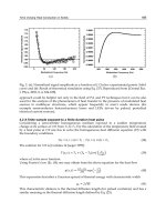
Fig. 7 shows the experimental results for thermal conductivity, λ, of frozen Yakutian alluvial
soils in the wide range of saturation moisture contents W
sat
. It should be noted that full
saturation was assumed in the experiments as a model of the natural state of permafrost
soils. As is seen, the dependence of λ on W
sat
differs between course- and fine-grained soils.
With increasing W
sat
, the thermal conductivity of the frozen sand at the point of full
saturation decreases, while that of the silt-clay increases tending to the thermal conductivity
of ice. The sand-silts are intermediate between these two soil types.
The observed differences in λ (W
sat
) can be explained by the differences in the unfrozen
water content and in the mineralogical composition of the soils. In the fine soils, the
unfrozen water content is quite high (about 0.1) at the measurement temperatures (about -
10°C). At low moisture contents, silt-clay can thus be considered as an unfrozen soil. The
effect of ice inclusions on overall heat conduction increases with increasing water content,
resulting in higher soil thermal conductivity. At high moisture contents, the thermal

conductivity of the silt-clay tends to that of ice. In the sands, the unfrozen water content is
low and the mineral particles are in direct contact with ice. As the mineral particles have a
higher thermal conductivity than ice, the thermal conductivity of the sand decreases with
increasing water (ice) content. The same is true for the unfrozen soils. The effect of the
unfrozen water film coating the mineral particles is less in the sand-silt compared to the silt-
clay. The thermal conductivity of the “mineral particle + unfrozen water” system is likely to
have the same values as for ice. The frozen saturated sand-silt has therefore a nearly
constant thermal conductivity over the entire range of saturation moisture contents. The
mineralogical composition has also an effect, resulting in an increase in the thermal
conductivity of solids from finer to coarser soils.
The above features of permafrost thermal conductivity can be estimated based on the
analytical theory of thermal conductivity of composite materials. The possible structural
models of soil follow from the mechanism of water binding by mineral particles. Soil
particles possess excess surface energy which depends on their size and mineral
composition. When water enters the ground, it interacts with the mineral particles under the
influence of molecular forces and surrounds them in concentric layers until the excess of
surface energy is removed. The particles interact through the bound water layer, forming a
stable system with dispersed particles. The remaining part of the soil pores is filled with free
water. As the soil temperature decreases, primarily near 0°C, the free water begins to freeze.
Then more of the bound water freezes with a further decrease in temperature. The strongly
bound water remains unfrozen down to about -20°C. When frozen, the system of dispersed
particles is cemented by ice, becoming even more stable. Hence, the thermal conductivity of
fine-grained permafrost soils at different subzero temperatures can be estimated considering
a three-component shell system (mineral particle + unfrozen water + ice) as shown in Fig. 8.
Mineral particles in this scheme are assumed to be spherical in shape.

Convection and Conduction Heat Transfer

248

Fig. 7. Thermal conductivity vs. saturation moisture content for alluvial sediments in frozen
state: 1 - sand; 2 – sand-silt; 3 – silt-clay; 4 - experimental curves; 5 – predicted curves


Fig. 8. Three-component shell medium: 1 – soil mineral particle; 2 – unfrozen water; 3 – ice
The effective conductivity λ of such a shell system can be predicted using the Maxwell
method based on the solution of Laplace’s equation for a medium with a constant
temperature gradient at a distance from the spherical particle with a shell. The equation has
the form (Belskaya, 1981)

(
)
(
)
()()
uw s uw i
uw i
uw s
i
uw s i uw
i
iuw
uw s
2
2
2
2
2
2
⎡

⎤
ελ −λ λ +λ
σλ −λ−
⎢
⎥
λ+λ
λ−λ
⎣
⎦
=
ελ −λ λ−λ
λ− λ
λ+λ +
λ+λ
, (32)
Analytical Methods for Estimating Thermal Conductivity
of Multi-Component Natural Systems in Permafrost Areas

249
where
33
suws
4R 4R
/
33
+
ππ
ε= is the volume fraction of the mineral soil solids in the two-
component system consisting of mineral solids and unfrozen water; σ is the volume fraction
of the mineral solids and unfrozen water in the soil; the subscripts “s”, “i” and “uw” refer to

the mineral solids, ice and unfrozen water, respectively.
Parameters
ε and
υ
in Eq. (32) can be expressed in terms of the volume fractions of soil
solids m
s
and unfrozen water m
uw


s
suw
m
mm
ε=
+
and
suw
mmσ= +

Considering the relation of m
s
and m
uw
to the saturation moisture content W
sat
and unfrozen
water content m
uw

s
s
sat s
m
1W
ρ
=
+
ρ
and
suw
uw
sat s
W
m
1W
ρ
=
+
ρ
,
(
s
ρ is the solids density), we finally obtain the following expression for the thermal
conductivity λ of a saturated frozen soil (Gavriliev, 1989):

i
N2М

N М
+
λ=λ
−
, (33)
where
N=
()
(
)
(
)
uw s i uw
sat s i uw
uw s uw s
2
1W 2
1W 2
⎡
⎤
λ−λλ−λ
+ρλ+λ+ ⋅
⎢
⎥
+ρ λ+λ
⎣
⎦
, (34)
M=
()()

(
)
(
)
uw s uw i
uw s uw i
uw s
2
1W
2
λ
−λ λ +λ
+ρλ−λ−
λ+λ
. (35)
In Eqs. (33) - (35), all limiting conditions are satisfied. At W
sat
→∞, λ=λ
i
. If W
sat
=0 and W
uw
=0,
then
λ=λ
s
. When W
uw
=0, the well-known Maxwell-Odolevsky equation for a two-

component medium is obtained, which can be expressed in terms of moisture content as

(
)
(
)
(
)
()()()
sat s i s s i
i
sat s i s s i
1W 2 2
1W 2
+
ρλ+λ+λ−λ
λ=λ
+
ρλ+λ−λ−λ
. (36)
Eq. (36) is also applicable to unfrozen soils, if the thermal conductivity of water
λ
w
is used
instead of
λ
i
.
The presence of entrapped air reduces the thermal conductivity of frozen soils, and this can
be expressed as:

(
)
()
s
ssat
21W
23WW
λ+ρ
λ=
+ρ −
, (37)
where W is the actual moisture content of the soil which should vary in the range

Convection and Conduction Heat Transfer

250
W≥
sat
moi s
0.4 0.4
1W
⎛⎞
−−
⎜⎟
ρ
ρ
⎝⎠
, (38)
where ρ

moi
is the parameter dependent on the soil condition which has a value of 1 above
0°C and 0.92 below 0°C.
The relation (38) may be particularly useful for estimating the thermal conductivity of the
thawed soils where any excess water escapes on thawing (if the thawing layer is not
underlain by frozen soil) and only part of the moisture is retained due to surface tension.
For actual computations, the values for thermal conductivity of soil constituents should be
specified in Eqs. (34) and (35). For pure ice at t = 0°C
λ = 2.25 W/(m•K). The thermal
conductivity of unfrozen water can be taken approximately equal to that of free, i.e.,
λ = 0.58
W/(m•K), since all anomalies in the properties of bound water are related to its strongly
adsorbed portion which is insignificant in amount. The thermal conductivity of mineral soil
solids depends on the mineral composition of particles and may be approximately estimated
by Eq. (14).
The distribution of minerals in soils is influenced by sedimentary conditions which vary
widely in nature. The amount of minerals in a soil can be estimated approximately based on
the relationship between particle mineralogy and size distribution. The three particle sizes
used for soil classification are clay (
< 0.002 mm), silt (0.002-0.05 mm), and sand (0.05-2.0
mm). In practice, it is assumed that the content of clay minerals, such as kaolinite, is equal to
the amount of clay-sized particles and 50% of silt-sized particles (Kokshenov, 1957). The
remainder of the soil consists predominantly of quartz and feldspar, and their relative
proportions vary widely depending on the soil origin. If no appropriate data are available,
the ratio of quartz to feldspar may be taken as 0.6:0.4 (Kokshenov, 1957).
In computations, the following values for
λ
j
may be used [W/(m•K)]: 6-7 for quartz, 1.9 for
feldspars, and 1.2 for kaolinite.

The distribution of particle sizes in a soil strongly depends on sedimentation conditions. If
no granulometric data are available, the values given in Table 1 may be used for
approximate estimations.

Particle size
Soil type
Clay Silt Sand
Sand 0.02 0.10 0.88
Sand-silt 0.06 0.30 0.64
Silt-clay 0.20 0.37 0.43
Table 1. Relative proportions of particles sizes in soils
Comparison of the predicted and experimental data (see Fig. 7) shows that Eqs. (33) - (35)
provide satisfactory results. The following values were used in the computations: for
λ
s

[W/(m•K)]:3.50 for sand, 2.70 for sand-silt, 2.30 for silt-clay; for W
uw
:0 for sand, 0.03 for
sand-silt and 0.10 for silt-clay.
5. Effect of organic matter on soil thermal conductivity
The unconsolidated soil layer on the immediate surface of the earth is enriched with organic
remains in the form of humus due to the effects of vegetation, animals (mainly
Analytical Methods for Estimating Thermal Conductivity
of Multi-Component Natural Systems in Permafrost Areas

251
microorganisms), climate, and human activity. The presence of organic matter has a strong
effect on the soil thermal properties.
Humic substances of the soil are specific high-molecular compounds. They play a significant

role in creating the soil structure (Tsyganov, 1958). The organic substances exist in the form
of very fine particles smaller than 0.2
μ referred to as colloids. Colloids have a very large
specific surface area that provides strong bonding of water in soil and the presence of large
amounts of unfrozen water at temperatures below freezing. Colloidal particles occur as sols
and gels. Sols are smaller particles which can aggregate into gels by coagulation. When
bound with water, organic particles form colloidal micelles having a core of an electrically
neutral mineral particle surrounded by ionic layers of adsorbed molecules of colloid
aggregate matter (hydrates: SiO2, Al2O3, MnO2, etc.) and electrolyte (water). At temperatures
below 0°C, the diffuse layer of water freezes, while the bound water remains unfrozen.
At the present stage of research, the problem of organic content effect on the thermal
conductivity of soils can only be approached using analytical methods, since there are
virtually no experimental data available.


Fig. 9. Schematic representation of the saturated frozen organic soil: 1 – mineral particle;
2 – colloid aggregate; 3 – unfrozen water; 4 - ice
Let us consider the saturated soils. Based on the above consideration, the saturated soil
containing organic matter can be represented as a four-component shell system within a
cubic cell (Fig. 9) consisting of a mineral particle (1), organic matter (humus) (2), unfrozen
water (3), and ice (4). The thermal conductivity of this system (frozen organic soil) calculated
with the successive use of Maxwell’s method is described by the equation (Gavrilyev, 2001)

(
)
i
f4
ii
3Z 1 m
1,

3Zm
⎡
⎤
−
λ=λ +
⎢
⎥
λ+
⎣
⎦
(39)
where

(
)
()
uw uw org i uw
uw i
uw i uw org uw
2mD Q31m2m
Z,
D31 m m m Q
λ+λ⎡−−⎤
⎣⎦
=
λ−λ
λ⎡−− ⎤+λ
⎣⎦
(40)

(
)
s org org s org
Dm 3mm,=λ +λ + (41)

Convection and Conduction Heat Transfer

252

(
)
org org s s org
Q2 m 3m m ,=λ +λ +
(42)
λ and m are the thermal conductivity and volume fractions of the components, respectively.
In the saturated unfrozen organic soil, the ice content m
i
is zero, and from Eq. (39) we obtain
the following equation for the thermal conductivity
t
λ


(
)
()
uw uw org uw
tuw
uw uw org uw
2mD Q32m

.
D3 m m Q
λ+λ−
λ=λ
λ−+λ
(43)
The volume fractions of the components of the organic soil in the saturated state, m
s
, m
org
,
m
uw
and m
i
, can be found using the following equations:

s
0
sat s
1
m,
1W
=
+
ρ
(44)

()
org s s

org
org org
nm
m,
1n
ρ
=
ρ−
(45)

uw uw d
mW,
=
γ (46)

(
)
isatuwd
mWW ,
=
−γ (47)

dssor
g
or
g
mm,
γ
=ρ +ρ (48)

sorguwi
mm m m1,
+
++=
(49)
where n
org
= P
org
/(P
s
+P
org
) is the relative weight of organic matter; Р
s
and Р
org
are the
weights of the soil mineral particles and organic matter in the dry state;
ρ is the unit weight
of the components;
0
sat
W is the saturation moisture content of the soil containing no organic
matter (fraction).
The saturation moisture content of the organic soil
sat
W is related to that of the soil
containing no organics
0

sat
W by the relationship:

()
org uw
0
sat sat org
org
n
WW1n .
ρ
=−−
ρ
(50)
For the saturated organic soil, the following relationship is valid:

s
d
sat s
,
1W
′
ρ
γ=
′
+
ρ
(51)
where
(

)
(
)
'
sssor
g
or
g
sor
g
mmmmρ=ρ +ρ +
is the unit weight of the organic soil.
In computations of the thermal conductivity of organic soils using Eqs. (39) - (43), the
following
λ values (W/(m•K)) can be taken for components: λ
org
=0.26 (Farouki 1986),
λ
uw
=0.58 and λ
i
=2.25. The value of λ
s
is a function of the soil type of the C horizon and can
be estimated from the mineral composition of the particles by Eq. (14).
Analytical Methods for Estimating Thermal Conductivity
of Multi-Component Natural Systems in Permafrost Areas

253
The λ

j
values of minerals are available in reference books (Birch, 1942; Clark, 1966;
Kobranova, 1962; Missenard, 1965; Smyslov et al., 1979). The unit weight of organic matter
(
ρ
org
) by analogy with peat (Gavriliev & Eliseev, 1970) can be taken as 1.48⋅10
3
kg/m
3
.
Fig. 10 shows the relationship between the thermal conductivity of a silt-clay [
λ
s
=2.50
W/(m•K)] and the saturation moisture content at different organic contents. It is seen that
reduction in the soil thermal conductivity due to the presence of organic matter is strongest
at low humus contents (n
org
< 0.1).


Fig. 10. Thermal conductivity of saturated silt-clay in frozen (solid lines) and thawed
(dashed lines) states vs saturation moisture content W
sat
at different organic contents n
org

(unit fraction): 1 - 0; 2 – 0.1; 3 – 0.2; 4 – 0.3
We note in conclusion that Eq. (39) can lead to Eq. (33) for permafrost with no second

component (m
org
=0).
6. Summary
Frozen soils are complex multi-component and multi-phase systems consisting of mineral
and organic particles, ice, unfrozen water, and gas (vapour). The specific conditions of
sedimentation and subsequent diagenesis in permafrost environments result in sediments of
permafrost-type with a very complex composition, structure and statistical particle
distribution.
A deep understanding of the thermal properties of frozen soils can only be gained through
an integral combination of experimental and analytical methods. Experimental methods
have limitations in quantitative terms. Having obtained some basic information with
experimental techniques, further in-depth study can be made using analytical methods. The
development of theoretical approach is needed to understand heat transfer processes and to
analyze experimental data on thermal properties of soils and rocks from a common point of
view.