Heat Conduction Basic Research Part 9 docx
Bạn đang xem bản rút gọn của tài liệu. Xem và tải ngay bản đầy đủ của tài liệu tại đây (582.59 KB, 25 trang )
Time Varying Heat Conduction in Solids
189
(a) (b)
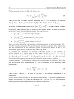
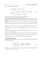
Fig. 2. (a): Normalized signal amplitude as a function of f. Circles: experimental points. Solid
curve and (b): Result of theoretical simulation using Eq. (37). Reproduced from [Central Eur.
J. Phys, 2010, 8, 4, 634-638].
approach could be helpful not only in the field of PA and PT techniques but it can be also
used for the analysis of the phenomenon of heat transfer in the presence of modulated heat
sources in multilayer structures, which appear frequently in men’s made devices (for
example semiconductor heterostructures lasers and LEDs driven by pulsed, periodical
electrical current sources).
4.2 A finite sample exposed to a finite duration heat pulse
Considering a semi-infinite homogeneous medium exposed to a sudden temperature
change at its surface at x=0 from T
0
to T
1
. For the calculation of the temperature field created
by a heat pulse at t=0 one has to solve the homogeneous heat diffusion equation (19) with
the boundary conditions
T(x = 0, t
0) = T
1
; T(x > 0, t=0) = T
0.
(38)
The solution for t>0 is [Carlslaw & Jaeger 1959]:
(
,
)
=
+
(
−
)
√
(39)
where erf is the error function.
Using Fourier’s law (Ec. (9)) one may obtain from the above equation for the heat flow
(
,
)
=
(
)
√
−
(40)
This expression describes a Gaussian spread of thermal energy with characteristic width
=2
√
(41)
This characteristic distance is the thermal diffusion length (for pulsed excitation) and has a
similar meaning as the thermal diffusion length defined by Eq. (23).
0 50 100 150 200
0.96
0.98
1.00
1.02
1.04
1.06
1.08
1.10
1.12
1.14
1.16
Normaliz ed Signal Am plitude
Modulation Frequency (Hz)
80 0 1 000 1200 140 0 16 00 1800
0. 99993
0. 99994
0. 99995
0. 99996
0. 99997
0. 99998
0. 99999
1. 00000
1. 00001
Norma liz ed S igna l Am plitude
Modulation Frequency (Hz)
Heat Conduction – Basic Research
190
If Eq. (40) is scaled to three dimensions one can show that after a time t has elapsed the heat
outspread over a sphere of radius
. Suppose that a spherical particle of radius R is heated in
the form described above by a heat pulse at its surface. The particle requires for cooling a
time similar to that the necessary for the heat to diffuse throughout its volume. The heat flux
at the opposite surface of the particle could be expressed as
(
=2
)
=
−
(42)
with q
0
as a time independent constant and a characteristic thermal time constant given by
=
(43)
This time depend strongly on particle size and on its thermal diffusivity,
[Greffet, 2007; Wolf,
2004; Marín, 2010]. As for most condensed matter samples the order of magnitude of
is 10
-6
m
2
/s, for a sphere of diameter 1 cm one obtain
c
=100 s and for a sphere with a radius of 6400
km, such as the Earth, this time is of around 10
12
years, both values compatible with daily
experience. But for spheres having diameters between 100 and 1 nm , these times values
ranging from about 10 ns to 1 ps, i.e. they are very close to the relaxation times,
, for which
Fourier’s Law of heat conduction is not more valid and the hyperbolic approach must be used
as well. The above equations enclose the basic principle behind a well established method for
thermal diffusivity measurement known as the Flash technique [Parker et al., 1961]. A sample
with well known thickness is rapidly heated by a heat pulse while its temperature evolution
with time is measured. From the thermal time constant the value of
can be determined
straightforwardly. Care must be taken with the heat pulse duration if the parabolic approach
will be used accurately. For time scales of the order of the relaxation time the solutions of the
hyperbolic heat diffusion equation can differ strongly from those obtained with the parabolic
one as has been shown elsewhere [Marín, et al.2005)].
Now, coming back to Eq. (40), one can see that the heat flux at the surface of the heated
sample (x=0) is
(
=0,
)
=
(
)
√
(44)
Thus the heat flow is not proportional to the thermal conductivity of the material, as under
steady state conditions (see Eq. (23)), but to its thermal effusivity [Bein & Pelzl, 1989].
If two
half infinite materials with temperatures T
1
and T
2
(T
1
>T
2
) touch with perfect thermal
contact at t=0, the mutual contact interface acquires a contact temperature T
c
in between.
This temperature can be calculated from Eq. (44) supposing that heat flowing out from the
hotter surface equals that flowing into the cooler one, i.e.
(
)
√
=
(
)
√
(45)
or
=
(46)
According to this result, if
1
=
2
, T
c
lies halfway between T
1
and T
2
, while if
1
>
2
, T
c
will be
closer to T
1
and if
1
<
2
, T
c
will be closer to T
2
. The Eq. (46) shows that our perception of the
Time Varying Heat Conduction in Solids
191
temperature is often affected by several variables, such as the kind of material we touch, its
absolute temperature and the time period of the “experiment”, among others (note that the
actual value of the contact temperature can be affected by factors such as objects surfaces
roughness that have not taking into account in the above calculations). For example, at room
temperature wooden objects feels warmer to the rapidly touch with our hands than those
made of a metal, but when a sufficient time has elapsed both seem to be at the same
temperature. Many people have the mistaken notion that the relevant thermophysical
parameter for the described phenomena is the thermal conductivity instead of the thermal
effusivity, as stated by Eq. (46). The source of this common mistake is the coincidence that in
solids, a high effusivity material is also a good heat conductor. The reason arises from the
almost constancy of the specific heat capacity of solids at room temperature explained at the
beginning of this section. Using Eq. (13) the Eq. (18) can be written as
2
=Ck. Then if
2
is
plotted as a function of k for homogeneous solids one can see that all points are placed close
to a straight line [Marín, 2007].
If we identify region 1 with our hand at T
1
=37
0
C and the other with a touched object at a
different temperature, T
2
, the contact temperature that our hand will reach upon contact can
be calculated using Eq. (46) and tabulated values of the thermal effusivities. Calculation of
the contact temperature between human skin at 37
0
C and different bodies at 20
0
C as a
function of their thermal effusivities show [E Marín, 2007] that when touching a high
thermal conductivity object such as a metal (e.g. Cu), as
metal
>>
skin
, the temperature of the
skin drops suddenly to 20
0
C and one sense the object as being “cold”. On the other hand,
when touching a body with a lower thermal conductivity, e.g. a wood’s object (
wood
<
skin
)
the skin temperature remains closest to 37
0
C, and one sense the object as being “warm”.
This is the reason why a metal object feels colder than a wooden one to the touch, although
they are both at the same, ambient equilibrium temperature. This is also the cause why
human foot skin feels different the temperature of floors of different materials which are at
the same room temperature and the explanation of why, when a person enters the cold
water in a swimming pool, the temperature immediately felt by the swimmer is near its
initial, higher, body temperature [Agrawal, 1999].
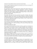
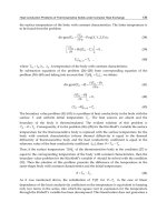
In Fig. 3 the calculated contact temperature between human skin at 37
0
C and bodies of
different materials at 1000
0
C (circles) and 0
0
C (squares) are represented as a function of their
thermal effusivities. One can see that the contact temperature tends to be, in both cases,
closer than that of the skin. This is one of the reasons why our skin is not burning when we
make a suddenly (transient) contact to a hotter object or freezing when touching a very cold
one (despite we fill that the object is hotter or colder, indeed).
Before concluding this subsection the following question merits further analysis. How long
can be the contact time,
l
, so that the transient analysis performed above becomes valid?
The answer has to do with the very well known fact that when the skin touches very hot or
cold objects a very thin layer of gas (with thickness L) is produced (e.g. water vapour
exhaled when the outer layers of the skin are heated or evaporated from ice when it is
heated by a warmer hand). This time can be calculated following a straightforward
calculation starting from Eq. (44) and Fourier´s law in the form given by Eq. (5). It lauds
[Marín ,2008]:
=
(47)
Heat Conduction – Basic Research
192
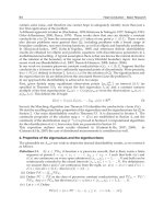
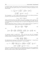
It is represented in Fig. (4) for different thicknesses of the gas (supposed to be air) layer
using for the skin temperature the value T
2
=37
0
C.
Fig. 3. Contact temperatures as a function of thermal effusivity calculated using Eq. (45)
when touching with the hand at 37
0
C objects of different materials at 0
0
C (circles) and
1000
0
C (squares). Reproduced with permission from [Latin American Journal of Physics
Education 2, 1, 15-17 (2008)]. Values of the thermal effusivities have been taken from
[Salazar, 2003]
Fig. 4. The time required for the skin to reach values of the contact temperature of 0
0
C and
100
0
C without frostbitten or burning up respectively (see text), as a function of the
hypothetical thickness of the gas layer evaporated at its surface. The solid and dotted curves
correspond to the case of touching a cold (-196
0
C) and a hot (600
0
C) object, respectively
Reproduced with permission from [Latin American Journal of Physics Education 2, 1, 15-17
(2008)].
The solid curve corresponds to the case of a cold touched object and the dotted line to that of
the hotter ones. For the temperature of a colder object the value T
1
=-196
0
C (e.g. liquid
01234567
37
38
39
40
41
42
43
44
Diamond
woodPVC
Glass
Pb
K
Ni
Co
Cu
T
C
(
0
C )
(x 10
4
J m
-2
K
-1
s
-1/2
)
0.0001 0.0010 0.0100
0.01
0.1
1
10
100
1000
l
(s)
L (m)
Time Varying Heat Conduction in Solids
193
Nitrogen) was taking. The corresponding limiting contact temperature will be T
c
=0
0
C (Eq.
(46)). In the case of the hot object the value T
1
=600
0
C (T
c
=100
0
C) was taking. From the figure
one can conclude that for gas layer thicknesses smaller than 1mm the time required to heat the
skin to 100
0
C by contact with an object at 600
0
C is lower than 3s, a reasonable value. On the
other hand, for the same layer thickness, liquid Nitrogen can be handled safely for a longer
period of time which, in the figure, is about 25 s. These times are of course shorter, because the
generated gas layers thicknesses are in reality much shorter than the here considered value.
The above examples try to clarify the role played by thermal effusivity in understanding
thermal physics concepts. According to the definition of thermal conductivity, under steady-
state conditions a good thermal conductor in contact with a thermal reservoir at a higher
temperature extracts from it more energy per second than a poor conductor, but under
transient conditions the density and the specific heat of the object also come into play
through the thermal effusivity concept. Thermal effusivity is not a well known heat
transport property, although it is the relevant parameter for surface heating or cooling
processes.
4.3 A finite slab with superficial continuous uniform thermal excitation
The following phenomenon also contradicts common intuition of many people: As a result
of superficial thermal excitation the front surface of a (thermally) thick sample reaches a
higher equilibrium temperature than a (thermally) thin one [Salazar et al., 2010; Marín et al.,
2011]. Consider a slab of a solid sample with thickness L at room temperature, T
0
, is
uniformly and continuously heated at its surface at x=0. The heating power density can be
described by the function:
=
0<0
>0
(48)
where P
0
is a constant.
The temperature field in a sample,
(
,
)
, can be obtained by solving the one-dimensional
heat diffusion problem (Eq. (19)) with surface energy losses, i.e., the third kind boundary
condition:
During heating the initial condition lauds
∆
↑
(
,=0
)
=
↑
(
,=0
)
−
=0 (49)
and the boundary conditions are:
∆
↑
(
0,
)
−
∆
↑
(
,
)
=
(50)
and
∆
↑
(
,
)
−
∆
↑
(
,
)
=0 (51)
The heat transfer coefficients at the front (heated) and at the rear surface of the sample have
been assumed to be the same and are represented by the variable H (see Eq. (7)).
When heating is interrupted, the equations (49) to (60) become
∆
↓
(
,=0
)
=
↓
(
,=0
)
−
=
(52)
Heat Conduction – Basic Research
194
∆
↓
(
0,
)
−
∆
↓
(
,
)
=0 (53)
and
∆
↓
(
,
)
−
∆
↓
(
,
)
=0 (54)
respectively, where T
eq
is the equilibrium temperature that the sample becomes when
thermal equilibrium is reached during illumination, being the initial sample temperature
when illumination is stopped.
The solution of this problem is [Valiente et al., 2006]
∆
↓
(
,
)
=−
∑
cos
+sin
(55)
and
∆
↑
(
,
)
=
(
/
)
+
∑
cos
+sin
(56)
where
= a
2
,
=
(57)
tan=
(58)
and
=−
‖
‖
(
)
()
(59)
with
‖
‖
=
cos
+sin
(60)
In order to examine under which condition a sample can be considered as a thermally thin
and thick slab the thermodynamic equilibrium limit must be analyzed, i.e. the limit of
infinitely long times.
Introducing the Biot Number defined in Eq. (8) and taking t after a straightforward
calculation the following results are obtained:
At x=0:
Δ
↑
(
0,∞
)
=
(61)
and
Δ
↑
(
,∞
)
=
(62)
Two limiting cases can be analyzed:
a. Very large Biot number (B
i
>>2):
Time Varying Heat Conduction in Solids
195
In this case Eq. (61) becomes
Δ
↑
(
0,∞
)
=
(63)
while from Eq. (62) one has
Δ
↑
(
,∞
)
=
(64)
For their quotient one can write
↑
(,)
↑
(,)
=
(65)
There is a thermal gradient across the sample so that the rear sample temperature becomes
k/LH times lower than the front temperature. Note that the temperature difference will
decrease as the heat losses do, as awaited looking at daily experience.
b. Very small Biot number (B
i
<<1):
In this case both Eq. (61) and Eq. (62) lead to
Δ
↑
(
0,∞
)
=Δ
↑
(
,∞
)
=
(66)
Thus, the equilibrium temperature becomes the same at both sample´s surfaces. The sample
can be considered thin enough so that there is not a temperature gradient across it. Thus, the
condition for a very thin sample is just:
≪1 (67)
With words, following the Biot´s number definition given in section 1, the temperature
gradient across the sample can be neglected when the conduction heat transfer through its
opposite surfaces of the samle is greater than convection and radiation losses.
The results presented above explain the phenomenon that the equilibrium temperature
becomes greater for a thicker sample. Denoting the front (heated side) sample´s temperature
of a thick sample (B
i
>> 1) at t as u
thick
, and that of a thin ones (B
i
<< 1) as u
thin
. Their
quotient is:
↑
(,)
↑
(,)
=2 (68)
Here L
thick
means that this is a thickness for which the sample is thermally thick. This means
that after a sufficient long time the front surface temperature of a thick sample becomes two
times higher than that for a thin sample. As discussed elsewhere [Marín et al., 2011]
The here presented results can have practical applications in the field of materials thermal
characterization. When the thermally thin condition is achieved, the rise temperature
becomes [Salazar et al., 2010; Valiente et al., 2006]
Δ
↑
=
1−−
(69)
while when illumination is interrupted the temperature decreases as
Δ
↓
=
−
(70)
where
Heat Conduction – Basic Research
196
=
/2 (71)
and L
thin
means that the sample thickness is such that it is thermally thin. If the front and/or
rear temperatures (remember that both are the same for a thermally thin sample) are
measured as a function of time during heating (and/or cooling) the value of
r
can be
determined by fitting to the Eq. (69) (and/or Eq. (70)) and then, using Eq. (71), the specific
heat capacity can be calculated if the sample´s thickness is known. This is the basis of the so-
called temperature relaxation method for measurement of C [Mansanares et al., 1990]. As we
see from Eq. (71) precise knowledge of H is necessary.
On the other hand, from Eq. (65) follows that measurement of the asymptotic values of rear
and front surface temperatures of a thermally thick sample leads to:
=
↑
(,)
↑
(,)
=
=
(72)
from which thermal conductivity could be determined. Note that the knowledge of the H
value is here necessary too.
From Eqs. (71) and (72) the thermal diffusivity value can be determined straightforwardly
without the necessity of knowing H, i.e. it can calculated from the quotient [Marín et al.,
2011]:
=
=2
(73)
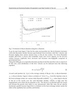
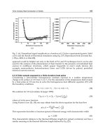
Fig. 5 shows a kind of Heisler Plot [Heisler, 1947] of the percentile error associated to the
thermally thick approximation as a function of the sample’s thickness using a typical value
of H=26 W/m
2
[Salazar et al., 2010] for a sample of plasticine (k=0.30 W/mK) and for a
sample of cork (k=0.04 W/mK).
Fig. 5. Heisler Plots for Plasticine (solid line) and Cork (dashed line).
0.00 0.02 0.04 0.06 0.08 0.10
1
10
10 0
Er ror ( % )
L
thick
(m)
Time Varying Heat Conduction in Solids
197
Note that for a 5 cm thick plasticine sample this error becomes about 20 %, while a
considerable decrease is achieved for a low conductivity sample such as cork with the same
thickness. These errors become lower for thicker samples, but rear surface temperature
measurement can become difficult. Thus it can be concluded that practical applications of
this method for thermal diffusivity measurement can be achieved better for samples with
thermal conductivities ranging between 10
-2
and 10
-1
W/mK. Although limited, in this range
of values are included an important class of materials such as woods, foams, porous
materials, etc. For these the thermally thick approximation can be reached with accuracy
lower than 10 % for thicknesses below about 2-3 cm.
Thermal diffusivity plays a very important role in non-stationary heat transfer problems
because its value is very sensible to temperature and to structural and compositional
changes in materials so that the development of techniques for its measurement is always
impetuous. The above described method is simple and inexpensive, and renders reliable
and precise results [Lara-Bernal et al., 2011]. The most important achievement of the
method is that it cancels the influence of the heat losses by convection and radiation
which is a handicap in other techniques because the difficulties for their experimental
quantification.
5. Conclusion
Heat conduction in solids under time varying heating is a very interesting and important
part of heat transfer from both, the phenomenological point of view and the practical
applications in the field of thermal properties characterization. In this chapter a brief
overview has been given for different kinds of thermal excitation. For each of them some
interesting physical situations have been explained that are often misinterpreted by a
general but also by specialized people. The incompatibility of the Fourier´s heat
conduction model with the relativistic principle of the upper limit for the propagation
velocity of signals imposed by the speed of light in vacuum was discussed, with emphasis
of the limits of validity this approach and the corrections needed in situations where it is
not applicable. Some applications of the thermal wave’s analogy with truly wave fields
have been described as well as the principal peculiarities of the heat transfer in the
presence of pulsed and transient heating. It has been shown that although the four
fundamental thermal parameters are related to one another by two equations, each of
them has its own meaning. While static and stationary phenomena are governed by
parameters like specific heat and thermal conductivity respectively, under non-stationary
conditions the thermal effusivity and diffusivity are the more important magnitudes.
While the former plays a fundamental role in the case of a body exposed to a finite
duration short pulse of heat and in problems involving the propagation of oscillating
wave fields at interfaces between dissimilar media, thermal diffusivity becomes the most
important thermophysical parameter to describe the mathematical form of the thermal
wave field inside a body heated by a non-stationary Source. It is worth to be noticed that
the special cases discussed here are not the only of interest for thermal science scientists.
There are several open questions that merit particular attention. For example, due to
different reasons (e.g. the use of synchronous detection in PT techniquess and
consideration of only the long-term temperature distribution once the system has
forgotten its initial conditions in the transient methods), in the majority of the works the
oscillatory part of the generated signal and the transient contribution have been analyzed
Heat Conduction – Basic Research
198
separately, with no attention to the combined signal that appears due to the well known
fact that when a thermal wave is switched on, it takes some time until phase and
amplitude have reached their final values. Nevertheless, it is expected that this chapter
will help scientists who wish to carry out theoretical or experimental research in the field
of heat transfer by conduction and thermal characterization of materials, as well as
students and teachers requiring a solid formation in this area.
6. Acknowledgment
This work was partially supported by SIP-IPN through projects 20090477 and 20100780, by
SEP-CONACyT Grant 83289 and by the SIBE Program of COFAA-IPN. The standing
support of J. A. I. Díaz Góngora and A. Calderón, from CICATA-Legaria, is greatly
appreciated. Some subjects treated in this chapter have been developed with the
collaboration of some colleagues and students. In particular the author is very grateful to A.
García-Chéquer and O. Delgado-Vasallo.
7. References
Agrawal D. C. (1999) Work and heat expenditure during swimming. Physics Education. Vol.
34, No. 4, (July 1999), pp. 220-225, ISSN 0031-9120.
Ahmed, E. and Hassan, S.Z. (2000) On Diffusion in some Biological and Economic systems.
Zeitschrift für Naturforshung. Vol. 55a, No. 8, (April 2000), pp. 669-672, ISSN 0932-
0784.
Almond, D. P. and Patel, P. M. (1996). Photothermal Science and Techniques in Physics and its
Applications, 10 Dobbsand, E. R. and Palmer, S. B. (Eds), ISBN 978-041-2578-80-9,
Chapman and Hall, London, U.K
Bein, B. K. and Pelzl, J. (1989). Analysis of Surfaces Exposed to Plasmas by Nondestructive
Photoacoustic and Photothermal Techniques, in Plasma Diagnostics, Vol. 2, Surface
Analysis and Interactions, pp. 211-326 Auciello, O. and Flamm D.L. (Eds.), ISBN 978-
012-0676-36-1, Academic Press, New York, U.S.A.
Band, W. and Meyer, L. (1948) Second sound and the heat conductivity in helium II, Physical
Review, Vol. 73, No. 3, (February 1948), pp. 226-229.
Bennett, C. A. and Patty R. R. (1982) Thermal wave interferometry: a potential application of
the photoacoustic effect. Applied Optics Vol. 21, No. 1, (January 1982), pp. 49-54,
ISSN 1559-128X
Boeker E and van Grondelle R (1999) Environmental Physics ISBN 978-047-1997-79-5, Wiley,
New York, U.S.A.
Caerels J., Glorieux C. and Thoen J. (1998) Absolute values of specific heat capacity and
thermal conductivity of liquids from different modes of operation of a simple
photopyroelectric setup. Review of Scientific Instruments. Vol. 69 , No. 6, (June 1998)
pp. 2452-2458, ISSN 0034-6748.
Carlslaw H. S. and Jaeger J. C. (1959) Conduction of Heat in Solids. ISBN 978-0198533030,
Oxford University Press, London, U.K.
Cattaneo, C. (1948) Sulla conduzione de calore, Atti Semin. Mat. Fis. Univ. Modena Vol. 3, pp.
83-101.
Time Varying Heat Conduction in Solids
199
Chen, Z. H., Bleiss, R. and Mandelis, A. (1993) Photothermal rate‐window spectrometry for
noncontact bulk lifetime measurements in semiconductors. Journal of Applied
Physics, Vol. 73, No. 10, (May 1993), pp. 5043-5048, ISSN 0021-8979
Cahill, D. G., Ford, W. K., Goodson, K. E., Mahan, G., Majumdar, D. A., Maris, H. J., Merlin,
R. and Phillpot, S. R. (2003) Nanoscale thermal transport. Journal of Applied Physics.
Vol. 93, No. 2, (January 2003), pp. 793-818, ISSN 0021-8979
Depriester M., Hus P., Delenclos S. and Hadj Sahraoiui A. (2005) New methodology for
thermal parameter measurements in solids using photothermal radiometry Review
of Scientific Instruments Vol 76, No. 7, (July 2005), pp. 074902-075100, ISSN 0034-
6748.
Fourier, J. (1878) The analytical theory of heat, Cambridge University Press, Cambridge,
U.K., Translated by Alexander Freeman. Reprinted by Dover Publications, New
York, 1955. French original: “Théorie analytique de la chaleur,” Didot, Paris,
1822.
Govender, M., Maartens, R. and Maharaj, S. (2001). A causal model of radiating stellar
collapse, Physics Letters A, Vol. 283, No. 1-2, pp. 71-79 (May 2001), ISSN: 0375-
9601.
Greffet, J. (2007) Laws of Macroscopic Heat Transfer and Their Limits in Topics in Applied Physics,
Voz, S. (Ed.) ISBN 978-354-0360-56-8, Springer, Paris, France, pp. 1-13
M P Heisler (1947) Temperature charts for induction and constant temperature heating.
Transactions of ASME, Vol. 69, pp. 227-236.
Ivanov R., Marin E., Moreno I. and Araujo C. (2010) Electropyroelectric technique for
measurement of the thermal effusivity of liquids. Journal of Physics D: Applied
Physics, Vol. 43, No. 22, pp. 225501-225506 (June 2010), ISSN 0022-3727.
Joseph, D. D. and Preziosi, L. (1989) Heat Waves. Reviews of Modern Physics. Vol. 61, No. 1,
(January-March), pp. 41-73, ISNN 0034-6861
Joseph, D. D. and Preziosi, L. (1990) Addendum to the paper “Heat Waves”. Reviews of
Modern Physics. Vol. 62, No. 2, (April-June 1990), pp. 375-391, ISNN 0034-6861
Landau, L. (1941) Theory of the Superfluidity of Helium II, Journal of Physics U.S.S.R. Vol.
5, No. 1, (January 1941), pp. 71-90, ISSN: 0368-3400.
Lara-Bernal et al. (2011) (submitted for publication).
Li, B., Xu, Y. and Choi, J. (1996). Applying Machine Learning Techniques, Proceedings of
ASME 2010 4th International Conference on Energy Sustainability, pp. 14-17, ISBN 842-
6508-23-3, Phoenix, Arizona, USA, May 17-22, 2010
C. A. S. Lima, L. C. M. Miranda and H. Vargas, (2006). Photoacoustics of Two‐Layer
Systems: Thermal Properties of Liquids and Thermal Wave Interference.
Instrumentation Science and Technology. Vol. 34, No. 1-2.,(February 2006), pp. 191-209
ISSN 1073-9149
Longuemart S., Quiroz A. G., Dadarlat D., Hadj Sahraoui A., Kolinsky C., Buisine J. M.,
Correa da Silva E., Mansanares A. M., Filip X., Neamtu C. (2002). An application of
the front photopyroelectric technique for measuring the thermal effusivity of some
foods. Instrumentation Science and Technology. Vol. 30, No. 2, (June 2002), pp. 157-
165, ISSN 1073-9149
Heat Conduction – Basic Research
200
Mandelis, A. (2000) Diffusion waves and their use. Physics Today Vol. 53, No. 8, (August
2000), pp. 29-36, ISSN 0031-9228.
Mandelis, A. and Zver, M. M. (1985) Theory of photopyroelectric spectroscopy of solids.
Journal of Applied Physics, Vol. 57, No. 9, (May 1985), pp. 4421-4431, ISSN 0021-
8979
Mansanares A.M., Bento A.C., Vargas H., Leite N.F., Miranda L.C.M. (1990) Phys Rev B Vol.
42, No. 7, (September 1990), pp. 4477-4486, ISSN 1098-0121.
Marín E., Marín-Antuña, J. and Díaz-Arencibia, P. (2002) On the wave treatment of the
conduction of heat in experiments with solids. European Journal of Physics. Vol. 23,
No. 5 (September 2002), pp. 523-532, ISSN 0143-0807
Marín, E., Marin, J. and Hechavarría, R., (2005) Hyperbolic heat diffusion in photothermal
experiments with solids, Journal de Physique IV, Vol. 125, No. 6, (June 2005), pp. 365-
368, ISSN 1155-4339.
Marín, E., Jean-Baptiste, E. and Hernández, M. (2006) Teaching thermal wave physics with
soils. Revista Mexicana de Física E Vol. 52, No. 1, (June 2006), pp. 21–27, ISSN 1870-
3542
Marin, E. (2007a) The role of thermal properties in periodic time-varying phenomena.
European Journal of Physics. Vol. 28, No. 3, (May 2007), pp. 429-445, ISSN 0143-
0807
Marín, E. (2007b) On the role of photothermal techniques for the thermal characterization of
nanofluids. Internet Electron. J. Nanoc. Moletrón. Vol. 5, No. 2, (September 2007), pp
1007-1014, ISSN 0188-6150.
Marín, E. (2008) Teaching thermal physics by Touching. Latin American Journal of Physics
Education Vol. 2, No. 1, (January 2008), pp. 15-17, ISSN 1870-9095
Marín, E. (2009a) Generalized treatment for diffusion waves. Revista Mexicana de Física. E.
Vol. 55, No. 1, (June 2009), pp. 85–91, ISSN 1870-3542.
Marín, E. (2009b) Basic principles of thermal wave physics and related techniques. ChapterI
in Thermal Wave Physics and Related Photothermal Techniques: Basic Principles
and Recent Developments. Marin, E. (Ed.) ISBN 978-81-7895-401-1, pp. 1-28 .
Transworld Research, Kerala, India.
Marín, E. (Ed.) (2009c) Thermal Wave Physics and Related Photothermal Techniques: Basic
Principles and Recent Developments. ISBN978-81-7895-401-1, Transworld Research,
Kerala, India.
Marín, E., Calderón, A. and Delgado-Vasallo, O. (2009) Similarity Theory and Dimensionless
Numbers in Heat Transfer, European Journal of Physics. Vol. 30, No. 3, (May 2009),
pp. 439-445, ISSN 0143-0807
Marin, E. (2010) Characteristic dimensions for heat transfer, Latin American Journal of Physics
Education. Vol. 4, No. 1, (January 2010), pp. 56-60, ISSN 1870-9095
Marin, E., García, A., Vera-Medina, G. and Calderón, A., (2010) On the modulation
frequency dependence of the photoacoustic signal for a metal coated glass-liquid
system. Central European Journal of Physics. Vol. 8, No. 4, (August 2010), pp. 634-638,
ISSN 1895-1082.
Marín, E., García, A., Juárez, G., Bermejo-Arenas, J. A. and Calderón, A., (2011)
On the
heating modulation frequency dependence of the photopyroelectric signal in
Time Varying Heat Conduction in Solids
201
experiments for liquid thermal characterization, Infrared Physics & Technology (in
press).
Marín, E., Lara-Bernal, A., Calderón, A. and Delgado-Vasallo O. (2011) On the heat
transfer through a solid slab heated uniformly and continuously on one of its
surfaces. European Journal of Physics. Vol. 32, No. 4, (May 2011), pp. 783–791, ISSN
0143-0807.
Narasimhan, T. N. (1999) Fourier´s heat conduction equation: History, influence, and
connections. Reviews of Geophysics. Vol. 37, No. 1, (February 199), pp. 151-172, ISSN
8755–1209.
Parker W. J., Jenkins, W. J., Butler, C. P., Abbott, G. L. (1961) Flash Method of Determining
Thermal Diffusivity, Heat Capacity and Thermal Conductivity. Journal of Applied
Physics Vol. 32, No. 9, (September 1961), pp. 1679-1684, ISSN 0021-8979
Peshkov, V. (1944) Second Sound in Helium II, Journal of Physics U.S.S.R. Vol. 8, No. 2,
(February 1944), pp. 381-383, ISSN: 0368-3400
Sahraoui, H. Longuemart, S., Dadarlat, D., Delenclos, S., Kolinsky C. and Buisine, J. M.
(2002) Review of Scientific Instruments Vol. 73, No. 7, (July 2002), pp. 2766-2771,
ISSN 0034-6748
Salazar, A. (2003) On thermal diffusivity European Journal of Physics. Vol. 24, No. 4, (July
2003), pp. 351-358, ISSN 0143-0807
Salazar, A. (2006), Energy propagation of thermal waves. European Journal of Physics. Vol. 27,
No. 6, (November 2006). pp. 1349-1356, ISSN 0143-0807
Salazar, A., Apiñaniz, E., Mendioroz, A., Aleaga, A. (2010) A thermal paradox: which gets
warmer? European Journal of Physics. Vol. 31 No. 5, (September 2010), pp. 1053-1060,
ISSN 0143-0807
Tisza, L. (1938) Sur la Supraconductibilit e thermique de l'helium II liquide et la statistique
de Bose-Einstein, Comptes Rendus de l'Académie des Sciences., Paris Vol. 207, pp.
1035-1038.
Tzou, D. Y. (1989) Schock wave formation around a moving heat source in a solid with finite
speed of heat propagation. International Journal of Mass and Heat Transfer. Vol. 32,
No. 10, (October 1989), pp. 1979-1987, ISSN 0017-9310
Tzou, D. Y. (1991) The resonance phenomenon in thermal waves. International Journal of
Engineering Science and Technology Vol. 29, No. 5, (May 1991), pp. 1167-1177 ISSN:
0975–5462
Valiente, H., Delgado-Vasallo, O., Abdelarrague, R., Calderón, A., Marín, E. (2006), Specific
Heat Measurements by a Thermal Relaxation Method: Influence of Convection and
Conduction. International Journal of Thermophysics Vol. 27, No. 6, (November 2006),
pp. 1859-1872, ISSN 0195-928X
Vargas, H. and Miranda, L.C.M. (1988) Photoacoustic and related photothermal
techniques. Physics Reports, Vol. 161, No. 2, (April 1988) pp. 43-101, ISSN: 0370-
1573
Vernotte, P. (1958) La véritable équation de la chaleur, Comptes Rendus de l'Académie des
Sciences, Paris Vol. 247, pp. 2103-2105.
Heat Conduction – Basic Research
202
Wautelet, M. and Duvivier, D. (2007) The characteristic dimensions of the nanoworld.
European Journal of Physics. Vol. 28, No. 5, (September 2007), pp. 953-960, , ISSN
0143-0807
Wolf, E. L. (2004) Nanophysics and Nanotechnology: An Introduction to Modern Concepts in
Nanoscience, ISBN 978-352-7406-51-7, Wiley-VCH, Weinheim, Germany.
Part 3
Coupling Between Heat Transfer and
Electromagnetic or Mechanical Excitations
0
Heat Transfer and Reconnection Diffusion in
Turbulent Magnetized Plasmas
A. Lazarian
Department of Astronomy, University of Wisconsin-Madison
USA
1. Introduction
It is well known that magnetic fields constrain motions of charged particles, impeding the
diffusion of charged particles perpendicular to magnetic field direction. This modification
of transport processes is of vital importance for a wide variety of astrophysical processes
including cosmic ray transport, transfer of heavy elements in the interstellar medium, star
formation etc. Dealing with these processes one should keep in mind that, in realistic
astrophysical conditions, magnetized fluids are turbulent. In this review we single out a
particular transport process, namely, heat transfer and consider how it occurs in the presence
of the magnetized turbulence. We show that the ability of magnetic field lines to constantly
change topology and connectivity is at the heart of the correct description of the 3D magnetic
field stochasticity in turbulent fluids. This ability is ensured by fast magnetic reconnection
in turbulent fluids and puts forward the concept of reconnection diffusion at the core of
the physical picture of heat transfer in astrophysical plasmas. Appealing to reconnection
diffusion we describe the ability of plasma to diffuse between different magnetized eddies
explaining the advection of the heat by turbulence. Adopting the structure of magnetic field
that follows from the modern understanding of MHD turbulence, we also discuss thermal
conductivity that arises as electrons stream along stochastic magnetic field lines. We compare
the effective heat transport that arise from the two processes and conclude that, in many
astrophysically-motivated cases, eddy advection of heat dominates. Finally, we discuss the
concepts of sub and superdiffusion and show that the subdiffusion requires rather restrictive
settings. At the same time, accelerated diffusion or superdiffusion of heat perpendicular to
the mean magnetic field direction is possible on the scales less than the injection scale of the
turbulence.
2. Main idea and structure of the review
Heat transfer in turbulent magnetized plasma is an important as trophysical problem which
is relevant to the wide variety of circumstancies from mixing layers in the Local Bubble (see
Smith & Cox 2001) and Milky way (Begelman & Fabian 1990) to cooling flows in intracluster
medium (ICM) (Fabian 1994). The latter problem has been subjected to particular scrutiny
as observations do not support the evidence for the cool gas (see Fabian et al. 2001). This is
suggestive of the existence of heating that replenishes the energy lost via X-ray emission. Heat
transfer from hot outer regions is an important process to consider in this context.
It is well known that magnetic fields can suppress thermal conduction perpendicular to their
direction. However, this is true for laminar magnetic field, while astrophysical plasmas are
9
2 Will-be-set-by-IN-TECH
generically turbulent (see Armstrong et al 1994, Chepurnov & Lazarian 2010). The issue of
heat transfer in realistic turbulent magnetic fields has been long debated ( see Bakunin 2005
and references therein).
Below we argue that turbulence changes the very nature of the process of heat transfer.
To understand the differences between laminar and turbulent cases one should consider
both motion of charged particles along turbulent magnetic fields and turbulent motions of
magnetized plasma that also transfer heat. The description of both processes require the
knowledge of the dynamics of magnetic field lines and the structure of the magnetic field lines
in turbulent flows. The answers to these questions are provided by the theories of magnetic
reconnection and magnetic turbulence. To provide the quantitative estimates of the heat
transfer the review addresses both theories, discussing the generic process of reconnection
diffusion which describes the diffusion induced by the action of turbulent motions in the
presence of reconnection. We stress the fundamental nature of the process which apart from
heat transfer is also important e.g. for removing magnetic field in star formation process
(Lazarian 2005).
In §2 we discuss the omnipresence of turbulence in astrophysical fluids, introduce major ideas
of MHD turbulence theory and turbulent magnetic reconnection in §3 and §4, respectively,
relate the concept of r econnection diffusion to the processes of heat transfer in magnetized
plasmas in §5. We provide detailed discussion of heat conductivity via streaming electrons in
§6, consider heat advection by turbulent eddies in §7, and compare the efficiencies of the latter
two processes in §8. Finally, w e discuss h eat transfer on scales smaller than the turbulence
injection scale in §9 and provide final remarks in §10.
3. Magnetized turbulent astrophysical media
Astrophysical plasmas are k nown to be magnetized and turbulent. Magnetization of these
fluids most frequently arises from the dynamo action to which turbulence is an essential
component (see Schekochihin et al. 2007). In fact, it has been shown that turbulence in
weakly magnetized conducting fluid converts about ten percent of the energy of the cascade
into the magnetic field (see Cho e t al. 2009). This fraction does not depend on the original
magnetization and therefore magnetic fields will come to equipartition with the turbulent
motions in about 10 eddy turnover times.
We deal with magnetohydrodynamic (MHD) turbulence which provides a correct fluid-type
description of plasma turbulence at large scales
1
. Astrophysical turbulence is a direct
consequence of large scale fluid motions experiencing low friction. This quantity is described
by Reynolds number Re
≡ LV /ν,whereL is the s cale of fluid motions, V is the velocity at this
scale and ν is fluid viscosity. The Reynolds numbers are typically very large in astrophysical
flows as the scales are large. As magnetic fields decrease the viscosity for the plasma motion
perpendicular to their direction, Re numbers get really astronomically large. For instance, Re
numbers of 10
10
are very common for astrophysical flow. For so large Re the inner degrees of
fluid motion get excited and a complex pattern of motion develops.
The drivers of turbulence, e.g. supernovae explosions in the interstellar medium, inject energy
at large scales and then the energy cascades down to small scales through a hierarchy of eddies
spanning up over the entire inertial range. The famous Kolmogorov picture (Kolmogorov
1941) corresponds to hydrodynamic turbulence, but, as we discuss further, a qualitatively
similar turbulence also develops in magnetized fluids/plasmas.
1
It is possible to show that in terms magnetic field wandering that is important, as we see below, for heat
transfer the MHD description is valid in collisionless regime of magnetized plasmas (Eyink, Lazarian
& V ishniac (2011).
206
Heat Conduction – Basic Research
Heat Transfer and Reconnection Diffusion in Turbulent Magnetized Plasmas 3
Simulations of interstellar medium, accretion disks and other astrophysical environments also
produce turbulent picture, provided that the simulations are not dominated by numerical
viscosity. The latter requirement is, as we see below, is very important for the correct
reproduction of the astrophysical reality with computers.
The definitive confirmation of turbulence presence comes from observations, e.g. observations
of electron density fluctuations in the interstellar medium, which produce a so-called Big
Power Law in the Sky (Armstrong et al. 1994, Chepurnov & Lazarian 2010), with the spectral
index coinciding with the Kolmogorov one. A more direct piece of evidence comes from
the observations of spectral lines. Apart from showing non-thermal Doppler broadening,
they also reveal spectra of supersonic turbulent velocity fluctuations when analyzed with
techniques like Velocity Channel Analysis (VCA) of Velocity Coordinate Spectrum (VCS)
developed (see Lazarian & Pogosyan 2000, 2004, 2006, 2008) and applied to the observational
data (see Padoan et al. 2004, 2009, Chepurnov et al. 2010) rather recently.
All in all, the discussion above was aimed at conveying the message that the turbulent state
of magnetized astrophysical fluids is a rule and therefore the discussion of any properties
of astrophysical systems should take this state into account. We shall show below that
both magnetic reconnection and heat transfer in magnetized fluids are radically changed by
turbulence.
4. Strong and weak Alfvenic turbulence
For the purposes of heat transfer, Alfvenic perturbations are most important. Numerical
studies in Cho & Lazarian (2002, 2003) showed that the Alfvenic turbulence develops
an independent cascade which is marginally affected by the fluid compressibility. This
observation corresponds to theoretical expectations of the Goldreich & Sridhar (1995) theory
that we briefly describe below (see also Lithwick & Goldreich 2001). In this respect we
note that the MHD approximation is widely used to describe the actual magnetized plasma
turbulence over scales that are much larger than both the mean free path of the particles and
their Larmor radius (see Kulsrud 2004 and ref. therein). More generally, the most important
incompressible Alfenic part of the plasma motions can described by MHD even below the
mean free path (see Eyink et al. 2011 and ref. therein).
While having a long history of ideas, the theory of MHD turbulence has become testable
recently due to the advent numerical simulations (see Biskamp 2003) which confirm (see
Cho & Lazarian 2005 and ref. therein) the prediction of m agnetized Alfvénic eddies be ing
elongated in the direction of magnetic field (see Shebalin, Matthaeus & Montgomery 1983,
Higdon 1984) and provided results consistent with the quantitative relations for the degree of
eddy elongation obtained in Goldreich & Sridhar (1995, henceforth GS95).
The hydrodynamic counterpart of the MHD turbulence theory is the famous Kolmogorov
theory of turbulence. In that theory, energy is injected at large scales, creating large eddies
which correspond to large Re numbers and therefore do not dissipate energy through
viscosity
2
but transfer energy to smaller eddies. The process continues till the cascade reaches
the eddies that are small enough to dissipate energy over an eddy turnover time. In the
absence of compressibility the hydrodynamic cascade of energy is
∼ v
2
l
/τ
casc,l
= con st,where
v
l
is the velocity at the scale l and the cascading time for the eddies of size l is τ
cask,l
≈ l/v
l
.
From this the well known relation v
l
∼ l
1/3
follows.
2
Reynolds number Re ≡ LV/ν =(V/L)/(ν/L
2
) which is the ratio of the eddy turnover rate
τ
−1
eddy
= V/L and the viscous dissipation rate τ
−1
dis
= η/L
2
. Therefore large Re correspond to negligible
viscous dissipation of large eddies over the cascading time τ
casc
which is equal to τ
eddy
in Kolmogorov
turbulence.
207
Heat Transfer and Reconnection Diffusion in Turbulent Magnetized Plasmas
4 Will-be-set-by-IN-TECH
Modern MHD turbulence theory can also be understood in terms of eddies. However, in the
presence of dynamically important magnetic field, eddies cannot b e isotropic. Any motions
bending magnetic field should induce a back-reaction and Alfven waves propagating along
the magnetic field. At the same time, one can imagine eddies mixing magnetic field lines
perpendicular to the direction of magnetic field. For the latter eddies the original Kolmogorov
treatment is applicable resulting perpendicular motions scaling as v
l
l
1/3
⊥
,wherel
⊥
denotes
scales measured perpendicular to magnetic field and correspond to the perpendicular size of
the eddy. These mixing motions induce Alfven waves which determine the parallel size of the
magnetized eddy. The key stone of the GS95 theory is critical balance, i.e. the equality of the
eddy turnover time l
⊥
/v
l
and the period of the corresponding Alfven wave ∼ l
/V
A
,where
l
is the parallel eddy scale and V
A
is the Alfven velocity. Making use of the earlier expression
for v
l
one can easily obtain l
∼ l
2/3
⊥
, which reflects the tendency of eddies to become more
and more elongated as energy cascades to smaller scales.
While the arguments above are far from being rigorous they correctly reproduce the basic
scalings of magnetized turbulence when the velocity equal to V
A
at the injection scale L.The
most serious argument against the picture is the ability of eddies to perform mixing motions
perpendicular to magnetic field. We shall address this issue in §3 but for now we just mention
in passing that strongly non-linear turbulence does not usually allow the exact derivations. It
is numerical experiments that proved the above scalings for incompressible MHD turbulence
(Cho & Vishniac 2000, Maron & Goldreich 2001, Cho, Lazarian & Vishniac 2002) and for the
Alfvenic component of the compressible MHD turbulence (Cho & Lazarian 2002, 2003, Kowal
& Lazarian 2010).
It is important to stress that the scales l
⊥
and l
are measured in respect to the system
of reference related to the direction of the local magnetic field "seen" b y the eddy. This
notion was not present in the original formulation of the GS95 theory and was added in
Lazarian & Vishniac (1999) (see also Cho & Vishniac 2000, Maron & Goldreich 2001, Cho et
al. 2002). In terms of mixing motions that we mentioned above it is rather obvious that the
free Kolmogorov-type mixing is possible only in respect to the local magnetic field of the eddy
rather than the mean magnetic field of the flow.
GS95 theory assumes the isotropic injection of energy at scale L and the injection velocity equal
to the Alfvén velocity in the fluid V
A
, i.e. the Alfvén Mach number M
A
≡ (δV/V
A
)=1. This
model can be easily generalized for both M
A
< 1andM
A
> 1 at the injection (see Lazarian &
Vishniac 1999 and Lazarian 2006, respectively). Indeed, if M
A
> 1, instead of the driving scale
L for one can use another scale, namely l
A
, which is the scale at which the turbulent velocity
gets equal to V
A
.ForM
A
1 magnetic fi elds are not dynamically important at the largest
scales and the turbulence at those scales follows the isotropic Kolmogorov cascade v
l
∼ l
1/3
over the range of scales [L, l
A
].Thisprovidesl
A
∼ LM
−3
A
.IfM
A
< 1, the turbulence obeys
GS95 scaling (also called “strong” MHD turbulence) not from the scale L, but from a smaller
scale l
trans
∼ LM
2
A
(Lazarian & Vishniac 1999), while in the range [L, l
trans
] the turbulence is
“weak”.
The properties of weak and strong turbulence are rather different. The weak turbulence
is wave-like turbulence with wave packets undergoing many collisions before transferring
energy to small scales
3
. On the contrary, the strong turbulence is eddy-like with cascading
happening similar to Kolmogorov turbulence within roughly an eddy turnover time. One
also should remember that the notion "strong" should not be associated with the amplitude
of turbulent motions, but o nly with the strength of the non-linear interaction. As the weak
3
Weak turbulence, unlike the strong one, allows an exact analytical treatment (Gaultier et al. 2002).
208
Heat Conduction – Basic Research
Heat Transfer and Reconnection Diffusion in Turbulent Magnetized Plasmas 5
turbulence evolves, the interactions of wave packets increases as the ratio of the parallel to
perpendicular scales of the packets increases making the turbulence strong. I n this case, the
amplitude of the perturbations may be very small.
While the re ongoing debates whether the original GS95 theory should be m odified to better
describe MHD turbulence, we believe that, first of all, we do not have compelling evidence
that GS95 is not adequate
4
. Moreover, the proposed additions to the GS95 model do not
change the nature of the physical processes that we present below.
The quantitative picture of astrophysical turbulence sketched in this section gives us a way to
proceed with the quantitative description of key processes necessary to describe heat transfer.
The interaction of fundamental MHD modes within the cascade of compressible magnetized
turbulence is described in Cho & Lazarian (2005), but this interaction is not so important for
the processes of heat transfer that we discuss below.
5. Magnetic reconnection of turbulent magnetic flux
Magnetic re connection is a fundamental process that violates magnetic flux being frozen i n
within highly conductive fluids. Intuitively one may expect that magnetic fields in turbulent
fluids cannot be perfectly frozen in. Theory that we describe below provide quantitative
estimates of the violation of frozen in condition within turbulent fluids.
We would like to stress that the we are discussing the case of dynamically important magnetic
field, including the case of weakly turbulent magnetic field. The case of weak magnetic field
which can be easily stretched and bended by turbulence at any scale up to the dissipation one
is rather trivial and of little astrophysical significance
5
. At the same time, at sufficiently small
scales magnetic fields get dynamically important even for superAlfvenic turbulence.
Within the picture of eddies mixing perpendicular to the local magnetic field that we
provided in the previous section, it is suggestive that magnetized eddies can provide
turbulent advection of heat similar to the ordinary hydrodynamic eddies. This is rather
counter-intuitive notion in view of the well-entrenched idea of flux being frozen in
astrophysical fluids. As it is e xplained in Eyink et al. ( 2011) the frozen-in condition is not
a good approximation for the turbulent fluids
6
. The violation of the perfect frozenness of the
magnetic field in plasmas also follows from LV99 model of reconnection (see discussion in
Vishniac & Lazarian 1999).
A picture of two flux tubes of different d irections which get into contact in 3D space is the
generic framework to describe magnetic reconnection. The upper panel of Figure 1 illustrates
why reconnection is so slow in the textbook Sweet-Parker model. Indeed, the model considers
magnetic fields that are laminar and therefore the frozen-in condition for magnetic field
is violated only over a thin layer dominated by plasma resistivity. The scales over which
the resistive diffusion is important are microscopic and therefore the layer is very thin, i.e.
Δ
L
x
,whereL
x
is the scale at which magnetic flux tubes come into contact. The latter
4
Recent work by Beresnyak & Lazarian (2010) shows that present day numerical simulations are unable
to reveal the actual inertial range of MHD turbulence making the discussions of the discrepancies of the
numerically measured spectrum and the GS95 predictions rather premature. In addition, new higher
resolution simulations by Beresnyak (2011) reveal the predicted
−5/3 spectral slope.
5
In the case of dynamically unimportant field, the magnetic dissipation and reconnection happens on
the scales of the Ohmic diffusion scale and the effects of magnetic field on the turbulent cascade are
negligible. However, turbulent motions transfer an appreciable portion of the cascading energy into
magnetic energy (see Cho et al. 2010). As a result, the state of intensive turbulence with negligible
magnetic field is short-lived.
6
Formal mathematical arguments on how and why the frozen-in condition fails may be found in Eyink
(2011).
209
Heat Transfer and Reconnection Diffusion in Turbulent Magnetized Plasmas
6 Will-be-set-by-IN-TECH
Δ
Δ
λ
λ
x
L
Sweet−Parker model
Turbulent model
blow up
Fig. 1. Upper panel: Sweet-Parker reconnection. Δ is limited by resistivity and small. Middle
panel: reconnection according to LV99 model. Δ is determined by turbulent field wandering
and can be large. Lower panel: magnetic field reconnect over small scales. From Lazarian,
Vishniac & Cho (2004).
is of the order of the diameter of the flux tubes and typically very large for astrophysical
conditions. During the process of magnetic reconnection all the plasma and the shared
magnetic flux
7
arriving over an astrophysical scale L
x
should be ejected through a microscopic
slot of thickness Δ. As the ejection velocity of magnetized plasmas is limited by Alfven
velocity V
A
, this automatically means that the velocity in the vertical direction, which is
reconnection velocity, is much less than V
A
.
The LV99 model generalizes the Sweet-Parker one by accounting for the existence of magnetic
field line stochasticity (Figure 1 (lower panels)). The depicted turbulence is sub-Alfvenic
with relatively small fluctuations of the magnetic field. At the same time turbulence induces
magnetic field wandering. This wandering was quantified in LV99 and it depends on the
intensity of turbulence. The vertical e xtend of wandering o f magnetic field lines that at any
point get into contact with the field of the other flux tube was identified in LV 99 wi th the
width of the outflow region. Note, that magnetic field wandering is a characteristic feature of
magnetized turbulence in 3D. Therefore, generically in turbulent reconnection the outflow is
no more constrained by the narrow resistive layer, but takes place through a much wider area
Δ defined by wandering magnetic field lines. The extend of field wandering determines the
reconnection velocity in LV99 model.
An important consequence of the LV99 reconnection is that as turbulence amplitude increases,
the outflow region and therefore reconnection rate also increases, which entails the ability of
7
Figure 1 presents only a cross section of the 3D reconnection layer. A shared component of magnetic
field is going t o be present in the generic 3D configurations of reconnecting magnetic flux tubes.
210
Heat Conduction – Basic Research
Heat Transfer and Reconnection Diffusion in Turbulent Magnetized Plasmas 7
reconnection to change its rate depending on the level of turbulence. The latter is important
both for understanding the dynamics of magnetic field in turbulent flow and f or explaining
flaring reconnection events, e.g. solar flares.
We sh ould note that the magnetic fie ld wandering is m ostly due to Alfvenic turbulence. To
describe the field wondering for weakly turbulent case LV99 extended the GS95 model for
a subAlfvenic case. The same field wandering
8
, as we discuss later, is important for heat
transfer by electrons streaming along magnetic field lines.
The predictions of the turbulent reconnection rates in LV99 were successfully tested 3D
numerical simualtions in Kowal et al. (2009) (see also Lazarian et al. 2010 for an example
of higher resolution runs). This testing provided stimulated work on the theory applications,
e.g. its implication for heat transfer. One should keep in mind that the LV model assumes that
the magnetic field flux tubes can come at arbitrary angle, which corresponds to the existence
of shared or guide field within the reconnection layer
9
.
Alternative models of magnetic reconnection appeal to different physics to overcome the
constraint of the Sweet-Parker model. In the Petcheck (1964) model of reconnection the
reconnection layer opens up to enable the outflow which thickness does not depend on
resistivity. To realize this idea inhomogeneous resistivity, e.g. anomalous resisitivity
associated with plasma effects, is required (see Shay & Drake 1998). However, for turbulent
plasmas, the effects arising from modifying the local reconnection events by introducing
anomalous resistivity are negligible as confirmed e.g. in Kowal et al. (2009). Other effects, e.g.
formation and ejection of plasmoids (see Shibata & Tanuma 2001, Lorreiro et al. 2008) which
may be important for initially laminar environments are not likely to play the dominant role
in turbulent plasmas either. Therefore in what follows dealing with turbulent transfer of hear
we shall appeal to the LV99 model of reconnection.
6. Reconnection diffusion and heat transfer
In the absence of the frozen-in condition in turbulent fluids one can talk about reconnection
diffusion in magnetized turbulent astrophysical plasmas. T he concept of reconnection
diffusion is based on LV99 model and was first discussed in Lazarian (2005) in terms of
star formation
10
. However, reconnection diffusion is a much broader concept applicable to
different astrophysical processes, including heat transfer in magnetized plasmas. In what
follows we shall discuss several processes that enable heat transfer perpendicular to the mean
magnetic field in the flow.
The picture frequently presented in textbooks may be rather misleading. Indeed, it is widely
assumed that magnetic field lines always preserve their identify in highly conductive plasmas
even in turbulent flows. In this s ituation the diffusion of charged particles perpendicular to
magnetic field lines is very restricted. For instance, the mass loading of magnetic field lines
8
As discussed in LV99 and in more details in Eyink et al. (2011) the magnetic field wandering, turbulence
and magnetic reconnection are very tightly related concepts. Without magnetic reconnection, properties
of magnetic turbulence and magnetic field wandering would be very different. For instance, in the
absence of fast reconnection, the formation of magnetic knots arising if magnetic fields were not able to
reconnect would destroy the self-similar cascade of Alfvenic turbulence. The rates predicted by LV99
are exactly the rates required to make Goldreich-Sridhar model of turbulence self-consistent.
9
The model in LV99 is three dimensional and it is not clear to what extend it can be applied to
2D turbulence (see discussion in ELV11 and references therein). However, the cases of pure 2D
reconnection and 2D turbulence are of little practical importance.
10
Indeed, the issue of flux being conserved within the cloud presents a problem for collapse of clouds
with strong magnetic field. These clouds also called subcritical were believed to evolve with the rates
determined by the relative drift of neutrals and ions, i.e. the ambipolar diffusion rate.
211
Heat Transfer and Reconnection Diffusion in Turbulent Magnetized Plasmas
8 Will-be-set-by-IN-TECH
Fig. 2. Diffusion of plasma in inhomogeneous magnetic field. 3D magnetic flux tubes get into
contact and after reconnection plasma streams along magnetic field lines. Right panel:XY
projection before reconnection, upper panel shows that the flux tubes are at angle in X-Z
plane. Left Panel: after reconnection.
does not change to a high degree and density and magnetic field compressions follow each
other. All these assumptions are violated in the presence of reconnection diffusion.
We shall first illustrate the reconnection diffusion process showing how it allows plasma to
move perpendicular to the mean inhomogeneous magnetic field (see Figure 2). Magnetic flux
tubes with entrained plasmas intersect each other at an angle and due to reconnection the
identity of magnetic field lines change. Before the reconnection plasma pressure P
pl asma
in
the tubes is different, but the total pressure P
pl asma
+ P
magn
is the s a me for two tubes. After
reconnection takes place, plasma streams along newly formed magnetic field lines to equalize
the pressure along two new flux tubes. The diffusion of plasmas and magnetic field takes
place. The effect of this process is to make magnetic field and plasmas more homogeneously
distributed in the absence of the external fields
11
. In terms of heat transfer, the process mixes
up plasma at different temperatures if the temperatures of plasma volumes along different
magnetic flux tubes were different.
If turbulence had only one scale of motions its action illustrated by Figure 2 would create every
flux tube columns of hot and cold gas exchanging heat w ith each other through the diffusion
of charged particles along magnetic field lines. This is not the case, however, for a turbulence
11
If this process acts in thepresence of gravity, as this is the case of star formation, the heavy fluid (plasma)
will tend to get to the gravitating center changing the mass to flux ratio, which is important to star
formation processes. In other words, reconnection diffusion can do the job that is usually associated
with the action of ambipolar diffusion (see numerical simulations in Santos de Lima et al. (2010).
212
Heat Conduction – Basic Research
Heat Transfer and Reconnection Diffusion in Turbulent Magnetized Plasmas 9
Fig. 3. Exchange of plasma between magnetic eddies. Eddies carrying magnetic flux tubes
interact through reconnection of the magnetic field lines belonging to two different eddies.
This enables the exchange of matter between eddies and induces a sort of turbulent
diffusivity of matter and magnetic field.
with an extended inertial cascade. Such a turbulence would induce mixing depicted in Figure
2 on every scale, mixing plasma at smaller and smaller scales.
When plasma pressure along magnetic field flux tubes is the same, the connection of flux
tubes which takes place i n turbulent media as shown in Figure 3 is still important for h eat
transfer. The reconnected flux tubes illustrate the formation of the wandering magnetic field
lines along which electron and ions can diffuse transporting heat. For the sake of simplicity,
we shall assume that electrons and ions have the same temperature. In this situation, the
transfer of heat by ions is negligible and for the rest of the presentation we shall talk about the
transport of heat by electrons moving along wandering field lines
12
.
Consider the above process of reconnection diffusion in more detail. The eddies 1 and 2
interact through the reconnection of the magnetic flux tubes associated with eddies. LV99
model shows that in turbulent flo ws reconnection happens within one eddy tur nover time,
thus ensuring that magnetic field does not prevent free mixing motions of fluid perpendicular
to the local direction of magnetic field. As a result of reconnection, the tube 1
low
11
up
transforms into 2
low
12
up
and a tube 2
low
22
up
transforms into 1
low
21
up
. If eddy 1 was
12
This is true provided that the current of diffusing hot electrons is compensated by the current of
oppositely moving cold electrons, the diffusivity of electrons along wandering magnetic field lines
is dominant compared with the diffusivity and heat transfer by protons and heavier ions. If there is
no compensating current, electrons and ions are coupled by electric field and have to diffuse along
wandering magnetic fields together and at the same rate. This could be the case of diffusion of plasmas
into neutral gas. However, we do not discuss these complications here
213
Heat Transfer and Reconnection Diffusion in Turbulent Magnetized Plasmas