Convection and Conduction Heat Transfer Part 13 doc

17
Properties and Numerical
Modeling-Simulation of Phase Changes Material
Pavel Fiala, Ivo Behunek and Petr Drexler
Brno univerzity of technology, Faculty of electrical engineering and communication,
Department of theoretical and experimental electrical engineering, Kolejni 4, Brno
Czech Republic

1. Introduction
There exists a domain of models that is principially classified into the linear and non-linear
fields of modelling. In the field of non-linear modelling, significant progress has been made
since the 1960s thanks to the widespread and regularly available computer technology. This
dynamic development influenced a large number of problems including the description of
physical behaviour of non-trivial tasks. Non-linear models are solved in the material,
spatial, and time domains. However, certain non-linear model domains are not sufficiently
developed or regularly used for analysis of the more simple tasks. This group includes task
models using non-linear discontinuous characteristics of materials, which can be
exemplified by the change of state of a material during heating or cooling. In this section, we
would like to use several descriptive examples to expose the problem of thermal tasks
solution utilizing applied materials with a phase change (PCM) (Gille, T.; at al. 2007, Volle,
F. at al. 2010, Shi, L.P.; at al. 2006). These are mostly coupled tasks (Fiala,P. December 1998).
Within the specification of different aspects of the solution process, emphasis will be placed
on the final accuracy of the results of numerical analyses, and therefore (rather than focusing
on a complete description of the model) the text will accentuate problematic spots within the
solution of such tasks.
The PCM characteristics are demonstrated on the task of designing a low-temperature
accumulator, an efficient cooler of electronic components, and a separator of impurities in
an industrial oil emulsion.
1.1 Energy, transformation, accumulation
Within the last decade, scientific interest in the fields of basic and applied research has been
focused more intensively on the problem of increasing the share of renewable sources of

energy in total energy consumption per capita (Solar energy 2010). In this context, we have
seen major development in the field of energy harvesting (Murat Kenisarin, & Khamid
Mahkamov May 2006, John Greenman at al. May 2005, Junrui Liang & Wei-Hsin Liao 2010,
Vijay Raghunathan at al. April 2005, Jirku T at al. May 2010), or the acquirement of energy
from hitherto unused forms. The reason for such processes in technology naturally consists
in the fact that the reserves of classical primary sources of energy and fossil fuels (Behunek,
I. 2002, WORLD ENERGY STATISTICS from the IEA 2002) available to current industrial

Convection and Conduction Heat Transfer

350
society are limited. Moreover, such classification applies also to the possibilities of utilizing
the energy of water and wind.
A large number of countries have committed themselves to the reduction of greenhouse gas
emissions and the related increase of renewable sources of energy (Ministery of industry
and trade of Czech Republic, Stat energetic conception 2004, Ministery of industry and trade
of Czech Republic 2000) share in total energy consumption. However, the effort to comply
with these commitments may be realized in absurd ways such as an uncontrolled surge in
the number of constructed solar photovoltaic systems, which is further aggravated by the
related problem of their integration into the energy production system of a country, Fig. 1.


Fig. 1. A photovoltaic power plant design, the Czech Republic
One of the applicable alternative source solutions consist in utilizing solar radiation ( Solar
energy, 2010) within its entire spectrum. Among the advantages of this energy harvesting
method there are mainly the low cost of the impinging energy, the unimpeded availability
of the source in many regions of the Earth, and the polution-free operation. Conversely, the
related disadvantages can be identified in the low density of the impinging radiation power
flow in the visible and the near-visible spectrum (λ∈<440,780> nm), the comparatively low
efficiency of transformation into other forms of energy (considering the currently used

photovoltaic elements), and the fact that the cost of a produced energy unit is often rather
high when compared to other clean sources of electrical energy (such as nuclear power
plants) (Kleczek, J. 1981). In consequence of the uneven power flow density of the solar
source within the daily or yearly cycle and owing to weather changes, the solar energy
application method is affected by the problems of effective utilization, regulation in power
systems, and necessity of accumulating the energy acquired from solar radiation.
A feasible technique of energy accumulation seems to consist in direct exploitation of
physical effect of material properties as related to metals, liquids and gases (Gille, T. 2007,
Shi, L.P. 2006). Accumulators will facilitate power take-off during any time period
depending on the needs of the consumer or the power system operator, which provides for
the balance in the cost/power take-off relation within the required time interval. Thus, the
power distribution network stability will be improved, with substantial reduction of the
probability of black-out (Black-out 2003). There occurs the compensation of time
disproportion between the potential of the sources and the eletrical energy on the one hand
and the consumption in time and place on the other. Solar energy accumulation can be
technologically realized through a wide variety of methods; also, research in the field is

Properties and Numerical Modeling-Simulation of Phase Changes Material

351
being consistently developed (Juodkazis, Saulius; at al. November 2004, Zhen Ren at al.
Januar 2010, Liu, Y T.; at al. 2008 ).
Some of the proposed approaches are based on classical solutions. These include the
accumulation of energy utilizing the potential energy of mass in a gravitational field (water),
the kinetic energy of mass (flywheels), the non-linearities in the state of a mass phase – the
compression of gases. Another group of accumulators is based on the solution utilizing the
energy of an electromagnetic field. In this case, the most common is the application of
electric accumulators or microbiological systems [mikrobiolog akumulator]. Yet another one
of the fields to be quoted comprises energy accumulation using the properties of chemical
bonds of non-trivial chemical systems (the production of synthetic fuels), electrochemical

bonds, and the utilization of photochemical energy (the accumulation of low-potential heat
in solar-powered systems).
The process of designing chemical accumulator forms utilizes the physical effects of non-
linear behaviour of materials at phase changes. (Behunek,I. April 2004, Behunek I & Fiala P.
Jun 2007).
2. Heat accumulation
Principles are known (Baylin, F. 1979) for the utilization of characteristics of chemical-
physical effects, and in this context there exist four basic methods of thermal energy
accumulation. The first method consists in the utilization of specific thermal capacity of
substances (sensible heat), the second one is built on the application of change in the state of
substances (latent heat) , the third one lies in the thermochemical reaction, and the fourth
one applies the sorption and desorption of gas / water vapour.
Generally, the thermochemical reactions method provides a higher density of accumulated
energy than the sensible heat or phase change options (Mar, R.W. & Bramletta, T.T. 1980).
An endothermic reaction product contains energy in the form of a chemical bond that is
released retroactively during an exothermic reaction. The energy release occurs through the
action of a catalyst, which is a suitable characteristic for long-term accumulation. Other
advantages of thermochemical accumulation include the possibility of transporting the
products over long distances, the possibility of product storage at both low (with a low rate
of loss) and very high temperatures (Goldstein, M. 1961), the low cost, and the fact that
products of the reaction can be used as the medium in thermodynamic cycles (The
Australian National University 2004). Currently, research (Mar, R.W. 1978, Mar, R.W. 1980)
is conducted in this field. In order to accumulate energy, we can utilize heat balance at
sorption/desorption of moisture in the working substance. The difference with respect to
other types of heat accumulation consists in the fact that sorption does not directly depend
on the temperature,. but rather on relative humidity of the surrounding air. Therefore, the
described method of accumulation may be realized at a constant temperature, which is an
aspect utilizable in discharging the accumulator. In the progress of charging, relative
humidity of air is decreased to the required level through heating the air to achieve a higher
temperature (Close, D.J. & Dunkle, R.V. 1977, Verdonschet, J.K.M. 1981).

2.1 Classical heat accumulation methods
The classical accumulation of heat utilizes the so-called sensible heat of substances (Kleczek,
J., 1981) being the simplest one of all the methods, this approach was historically used in the
first place. Traditional materials applied for the accumulation of heat are water and gravel.

Convection and Conduction Heat Transfer

352
The weight and specific heat capacity of these materials indicate the accumulable quantity of
heat. This quantity is given by the calorimetric equation

2
1
d
T
T
QVcT
ρ
=
∫
(1)
where T
1
is the temperature at the beginning and T
2
the temperature at the end of charging.
2.2 Water heat reservoirs
If water is utilized in the process of accumulation, it is usually held in a suitable container
during heating (Garg, H.P., at al. 1985). Even though the applicaton of water has proved to
be advantageous in many respects, there are also many drawbacks, especially for the

preservation of low-potential heat. Water has the highest specific heat capacity of all known
substances (Vohlídal J. et al. 1999). It can be applied as an accumulation and working
medium (exchangers are not necessary); charging and discharging can be simulated in an
exact manner. If water is applied, heat storage or offtake causes temperature fluctuation and
the thermal potential is lost (namely the accumulator is charged at a sufficiently high input
temperature T, which is averaged in the reservoir to a mean temperature T
stř
and, during the
subsequent heat offtake, the original temperature T can not be reached) (Fisher L.S. 1976,
Lavan, Z. & Thomson, J. 1977). With water accumulators, liquid photothermal collectors
need to be applied; this means that expensive and rather complicated technologie and
installation methods are used as opposed to the hot air option) .
2.3 Gravel heat accumulators
For multi-day or seasonal accumulation (Behunek, I. April 2004), heat reservoris utilizing
gravel are preferred; here, the air used as the heating medium is heated in hot-air collectors.
This system eliminates some of the disadvantages of the previously described method. In
regular realizations, Figure 2, heat transfer by conduction is also minimal (the individual
gravel pieces touch one another only at the edges); here, however, the characteristics include
low heat capacity of the crushed stone (excessive dimensions of the reservoir) as well as a
very difficult (even impossible as per (Garg, H.P., et al. 1985 ) simulation of charging and
discharging.

hot
gravel
hot
gravel
cool
gravel
cool
gravel

gravel
thermal accumulation
heating

Fig. 2. Schematic description of a heat accumulator using gravel

Properties and Numerical Modeling-Simulation of Phase Changes Material

353
2.4 Utilizing the change of state in substances for the accumulation of heat
A prospective method of heat accumulation consists in utilizing the change of state of a
substance used in a heat reservoir. Such reservoir charges (fillings) are described by
the abbreviation PCM (Phase Change Material). According to Ehrenfest (Mechlova, E.,
Kostal, K. 1999), the changes of state are among the first type of phase changes, where the
change of internal energy and substance volume occurs through a jump. If specific melting
heat or solidification of the given substance is utilized, the calorimetry equation assumes the
form

e
m
0m
m
dd
T
T
TT
QVh VcT VcT
ρρρ
=Δ+ +
∫∫

(2)
where
ρ
is the density, V the volume, c the specific heat, Δh
m
the enthalpy, Q the heat, and
T
m
, T
e
the temperature according to Figure 3. If heat is supplied to the material, there occurs
the transformation from the liquid into the solid state. Phase transition appears when crystal
lattice is disrupted, namely when the amplitude of the crystal lattice particles oscillation is
comparable with relative distance between the particles. At this moment, the oscillation
energy rises above the value of the crystal binding energy, the bond is broken and the
crystal transforms into the liquid phase. However, if heat is removed from the substance,
there occurs the solidification (crystallization) of material. During crystallization, the orderly
motion of molecules gradually assumes the character of thermal oscillations around certain
middle positions, namely crystal lattice is formed. In pure crystalline substances, melting
and solidification proceed at a constant temperature T
m
, which does not vary during the
phase transition. In amorphous substances, the phase transition temperature is not constant
and the state change occurs within a certain range of temperatures, Figure 4. In simplified
terms for a macroscopic description of the numerical model, the phase change of a material
is understood as a state in which the material changes its physical characteristics on the
basis of variations (external) of its thermodanymic system. This state is often accompanied
by a nonlinear effect, Figure 3. The effect involves energy Q supplied to the thermodynamic
system of the material, temperature T, latent energy
Δ

Q necessary to change the
externalmacroscopic state of the material, initial state temperature T
0
, phase change
temperature T
m
, and temperature T
e
limiting the low-temperature mode.

Q (J)
Δ
Q
T (K)
Δ
T
phase- 1
T
0

T
m

phase- 2
T
e


Fig. 3. The PCM macroscopic characteristics

Convection and Conduction Heat Transfer

354
q (kWh m
-3
)
T (K)
20
CaCl
2
.6H
2
O
30
40
50
20
40 60
80
120
140
100
N
a
2
CO
3
.10H
2
O

N
a
2
HPO
4
.12H
2
O
gravel
H
2
O
parafin

Fig. 4. The course of accumulator charging with PCMs and classical materials

enclosures with PCM
inlet of air
heat insulation
outlet of air
(ventilators)
ducts with flaps
1. layer
2. layer
3. layer
4. layer
5. layer
6. layer
7. layer
8. layer

Fig. 5. Experimental model of a heat accumulator

Properties and Numerical Modeling-Simulation of Phase Changes Material

355
2.5 Requirements placed on the PCM, reservoirs and casings
PCM materials applicable for the accumulation of heat utilizing state change ought to meet
the following criteria (Behunek, I. 2002): Physical (a suitable phase diagram in the transition
area, a suitable phase transition temperature, small changes of volume during the change of
state, high density of the substance, supercooling tolerance, high specific melting heat, good
thermal conductivity), chemical (nonflammability, nontoxicity, chemical stability,
anticorrosive properties), economical (low asking price, availability, low cost of a suitable
accumulator). The structure of PCM reservoirs must conform to standard requirements
placed on thermal containers. In general, with respect to the provision of a suitable speed of
heat transfer, it is necessary to encase the actual PCM material and insert the resulting
containers that hold the PCM into an external envelope; this insertion should be realized in
such a way that, through its circulation, the heating medium ensures an optimum transfer of
heat energy in both directions (during charging and discharging), Figure 5.
Consequently, there exists substantial similarity to caloric reservoirs containing crushed
stone (aggregate) and therefore the rules governing the construction of these reservoirs can
be applied.
2.6 Basic classification of PCM materials
If we are to futher consider the properties of PCMs, it is necessary to describe their
minimum classicification and properties in phase changes, relation (3).
a.
The advantages of anorganic substances (GARG, H.P. et al. 1985, VENER, C. 1997) mainly
consist in the high value of specific melting heat, good thermal conductivity,

nonflammability, and low cost. The negative characteristics include corrosivity of the
substances to most metals, decomposition, loss of hygroscopic water, and the possibility
of supercooling.
Examples of anorganic PCMs are as follows:
CaCl
2
.6H
2
O, Na
2
SO
4
.10H
2
O, Na
2
CO
3
.10H
2
O, MgCl
2
.6H
2
O, CaBr
2
.6H
2
O, Mg(NO
3

)
2
.6H
2
O,
LiNO
3
.3H
2
O, KF.4H
2
O, Na
2
SO
4
.10H
2
O, Na
2
HPO
4
.12H
2
O.

() () ( )
teplo
222
nn
XY mHO XY pHO m pHO⋅←⎯⎯→⋅+− (3)

b.
Organic substances (GARG, H.P. et al. 1985, VENER, C. 1997) offer advantages such as a
high value of specific melting heat, chemical stability, elimination of supercooling, and
no corrosivity. The disadvantages consist in the inferior thermal conductivity, relatively
significant variations of volume during the change of state, flammability). Examples of
organic PCMs include paraffin, wax, polyethylene glycol, high-density polyethylene,
stearic acid (C
17
H
35
COOH), and palmitic acid (C
15
H
31
COOH).
c.
Other substances include compounds, combinations of amorphous and crystalline
substances, kombinace amorfních a krystalických látek, clathrates, and other items.
The advantage of low-potential heat accumulation in PCM application consists in the
variability. A comparison of PCM and classical materials together with a listing of several
PCMs (] LANE, G.A. 1983, FAVIER, A. 1999) is provided in Table 1. The elementary
reference quantity is the density of accumulated energy. We assume the initial charging
temperature as T
0
20 °C and the final termperature as T
e
50 °C. The course of accumulator
loading with various types of filling (charge) is shown in Figure 4; a realization example of a
PCM-based accumulator is provided in Figure 5.

Convection and Conduction Heat Transfer

356
Material used for accumulation
in heat reservoir
Accumulated energy
density q [kWh.m
-3
]
Water 34,5
Aggregate of stones 23,0
Paraffin 62,4
CaCl
2
. 6H
2
O 117,4
Na
2
CO
3
. 10H
2
O 131,7
Na
2
HPO
4
. 12H
2

O 134,7
Table 1. A comparison of accumulated energy density for different substances

20
22
24
26
28
30
32
34
36
38
40
0:00 0:21 0:43 1:04 1:26 1:48 2:09
čas [hodiny]
°C
5
10
15
20
25
30
35
40
0:00 0:36 1:12 1:48 2:24 3:00 3:36 4:12
čas [hodiny]
°C

Fig. 6. Phase changes of CaCl

2
.6H
2
O

20
22
24
26
28
30
32
34
36
38
40
0:00 0:28 0:57 1:26 1:55 2:24 2:52
čas [hodiny]
°C
27
28
29
30
31
32
33
34
0:00 0:07 0:14 0:21 0:28 0:36 0:43 0:50
čas [minuty]
°C

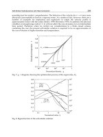
Fig. 7. Phase change of CaCl
2
.6H
2
O (CaCl
2
.4H
2
O crystallization)
2.7 Calcium chloride hexahydrate and its modification
In Figure 6, the phase change of CaCl
2
.6H
2
O during heating and cooling is shown. The
dashed lines show the theoretical behaviour under the condition when the melting and
freezing were realized at constant temperature T
m
– the case of pure crystallic substances.
Impurity and the methodology of measuring are the main cause of variations (the probe has
to be placed only in small amounts of hexahydrate. During solidification, ing occurred

Properties and Numerical Modeling-Simulation of Phase Changes Material

357
owing to weak nucleation. Crystallization was initiated thanks to a solid particle of the PCM
added to the measured sample. Otherwise, the crystallization would not have occurred. The
group of materials for the encasing of hexahydrate may include plastics, mild steel or
copper; aluminium or stainless steel are not suitable.

In some cases, temperature fluctuation above T
m
may occur during solidification (Figure 7).
The explanation was found in the binary diagram.
Figure 4 indicates the binary phase diagram of calcium chloride and water. The hexahydrate
contains 50,66 wt% CaCl
2
, and the tetrahydrate 60,63 wt%. The melting point of the
hexahydrate is 29,6 °C, with that of the tetrahydrate being 45,3 °C. The hexahydrate-α
tetrahydrate peritectic point is at 49,62 wt% CaCl
2
-50,38 wt% H
2
O, and 29,45 °C. In addition
to the stable form, there are two monotropic polymorphs of the tetrahydrate salt, β and γ.
The latter two are rarely encountered when dealing with the hexahydrate composition;
however, the α tetrahydrate is stable from its liquidus temperature, 32,78 °C, down to the
peritectic point, 29,45 °C, thus showing a span of 3,33 °C. When liquid CaCl
6
.6H
2
O is cooled
at the equilibrium, CaCl
2
.4H
2
O can begin to crystallize at 32,78 °C. When the peritectic is
reached at 29,45 °C, the tetrahydrate hydrates further to form hexahydrate, and the material
freezes. The maximum amount of tetrahydrate which can be formed is 9,45 wt%, calculated
by the lever rule. This process is reversed when solid CaCl

6
.6H
2
O is heated at the
equilibrium. At 29,45 °C the peritectic reaction occurs, forming 9,45% of CaCl
2
.4H
2
O and the
liquid of the peritectic composition. With increasing temperature, the tetrahydrate melts,
disappearing completely at 32,78 °C. Under actual freezing and melting conditions, the
equilibrium processes described above may occur only partially or not at all. Supercooling
of the tetrahydrate may lead to initial crystallization of the hexahydrate at 29,6 °C (or lower
if this phase also supercools). It is possible to conduct modification by additives. From a
number of potential candidates, Ba(OH)
2
, BaCO
3
and Sr(OH)
2
were chosen as they seemed
to be feasible. When we used Ba(OH)
2
and Sr(OH)
2
at 1% part by weight, there was no
supercooling. We were able to increase the stability of the equilibrium condition by adding
KCl (2 wt%) and NaCl, Figure 8. NaCl is a weak soluble in CaCl
2
.6H

2
O, therefore the part by
weight is only about 0,5%. The related disadvantage is that the melting point decreases by
ca. 3 °C at 26-27 °C.
2.8 Numerical model of heat accumulators
The effectivity of transferring the heat to active elements in the accumulator consists in the
optimum setting of dimensions and shapes in the process of circulation of the medium that
transfers energy in the accumulator. Therefore, a necessary precondition of the design
consisted in solving the air circulation model under the condition of change in its
temperature and thermodynamical variations in the PCM material. The actual model of
active elements and its temperature characteristic is not fundamental to this task; the
characteristic is known and realizable through commonly appplied methods.
A geometric model of one layer of the accumulator is shown in Figure 10 (Behunek, I. 2004)
It consists of 26 PVC pipes in a square configuration (Lienhard, J.H. IV & Lienhard, J.H. V.
2004). Inside of the pipes there are 9,36 litres of modified CaCl
2
.6H
2
O. The air flows through
the layer and transfers heat into the pipes. The related numerical solution was realized in
two parts. First, we solved the turbulence model and obtained the heat transfer film
coefficients. These results constituted the input for the solution of the second part namely
the calculation of the thermal model. The time dependence of temperature distribution in
the layer is the final result.

Convection and Conduction Heat Transfer

358

Fig. 8. Binary diagram of CaCl

2
.6H
2
O [9]

20
22
24
26
28
30
32
34
36
38
40
0:00 0:15 0:31 0:47 1:03 1:19 1:35 1:50 2:06 2:22
čas [hodiny]
°C
20
22
24
26
28
30
32
34
36
38
40

0:00 0:11 0:23 0:34 0:46 0:57 1:09 1:20 1:32 1:43
čas [hodiny]
°C

Fig. 9. Modification of CaCl
2
.6H
2
O at a different rate of heat removal

Properties and Numerical Modeling-Simulation of Phase Changes Material

359
CaCl

2

.

6

H

2
O
PVC pipe

air

750

6

0

0

direction of air flow
Ω
Γ
m

Γ
Air
Γ
PCM

100

Fig. 10. Geometric model of a layer with the mesh of elements
2.8.1 Mathematical and numerical model
The mathematical model of air velocity distribution uses fluid equations which were
derived for the incompressible fluid with the condition
0div
ν
=
(4)
For a steady state of flow there holds the continuity equation

0div

ρ
ν
=
(5)
We assume a turbulent flow
2curl w
ν
= (6)
where
ω
is the angular velocity of fluid. If we use the Stokes theorem, the Helmholtz
theorem for the moving particle and the continuity equation, we can formulate from the
equilibrium of forces the Navier-Stokes equation for the fluid element

vυAvv
v
Δ⋅+−=⋅+
∂
∂
pgradgrad
t
T
ρ
1
)(

(7)
where
A is the external acceleration,
υ

the vector of kinematic viscosity, and (grad v) has the
dimension of tensor. In equation (7) we substitute pressure losses

xx x xxx
yy y yyy
hh
zz z zzz
h
vvu vvu
vvu
ff
gradp K v v C v K v v C v
DD
f
Kv v Cv
D
ρρμ ρρμ
ρρμ
⎛⎞⎛ ⎞
=− + + − + +
⎜⎟⎜ ⎟
⎝⎠⎝ ⎠
⎛⎞
−++
⎜⎟
⎝⎠
(8)
where K are the suppressed pressure losses, f the resistance coefficient, D
h
the hydraulic

diameter of ribs, C the air permeability of system,
μ
the dynamic viscosity, and u
x,y,z
the unit
vector of the Cartesian coordinate system. The resistance coefficient is obtained from the
Boussinesq theorem

b
aRef
−
=

(9)

Convection and Conduction Heat Transfer

360
where Re is Reynolds number and a, b are coefficients from [40]. The model of short
deformation field is formulated from the condition of steady-state stability, which is
expressed

∫
Ω
=+
∫
0dd ΓΩ tf

(10)
where

f are the specific forces in domain Ω, and t the pressures, tensions and shear stresses
on the interface area Γ. By means of the transformation into local coordinates, we obtain the
differential form for the static equilibrium

0
v
2
=+ Tf div
(11)
where div
2
stands for the div operator of tensor quantity and T
v
is the tensor of internal
tension

⎥
⎥
⎥
⎦
⎤
⎢
⎢
⎢
⎣
⎡
=
zyx
zyx
zyx

v
ZZZ
YYY
XXX
T

(12)
where X, Y, Z are the stress components which act on elements of the area. It is possible to
add a form of specific force from (4)-(7) to the condition of static equilibrium. The form of
specific force is obtained by means of an external acceleration
A, on the condition that
pressure losses and shear stresses
τ
are given as

∑
=
=+−−
⎟
⎠
⎞
⎜
⎝
⎛
⋅⋅+
∂
∂
s
1
v

2
l
)(
N
l
T
divgrad
t
0TFAvv
v
ρρ
(13)
where
F
1
are the discrete forces and div
2
is the divergence operator of tensor. The model
which covers the forces, viscosity, and pressure losses is

()
s
l
1
v
vv A F v0
N
T
l
grad gradp

t
ρρμ
=
∂
⎛⎞
+
⋅⋅−−+−⋅Δ=
⎜⎟
∂
⎝⎠
∑
(14)
We can prepare the discretization of equation (7) by means of the approximation of velocity
v and acceleration a (Behunek I, Fiala P. Jun 2007). On the interface there are defined
boundary and initial conditions. Initial and boundary conditions can be written; the initial
temperature of the air is 50 °C, the initial velocity of the air is 0,4 m.s
-1
, the outlet pressure is
101,3 kPa + 10 Pa, and the initial temperature of the air inside the accumulator, PVC and
CaCl
2
.6H
2
O is 20 °C. There are the distribution of velocity values indicated in figures 11, 12,
and other results for the distribution of turbulent kinetic energy, dissipation, temperature
and pressure follow on Figures 13. Calculation of the thermal model (finite element methode
(FEM), finite volume methode (FVM), Ansys User’s Manual) was realized under the same
conditions as the previous turbulence model.
Figure 13 shows the time dependence of temperature in CaCl
2

.6H
2
O in the pipe marked
with a black cross (Figure 11). We can compare the result of the numerical simulation with
the measurement. Differences between the simulation and the measurement are caused by
the inaccuracy of the model with respect to reality.

Properties and Numerical Modeling-Simulation of Phase Changes Material

361

Fig. 11. Velocity distribution of the air


Fig. 12. Velocity distribution of the air (vectors, detail)


Fig. 13. Distribution of temperature

processor
ribs
PCM
Ω

Fig. 14. Example of a processor cooler with a phase change material)

Convection and Conduction Heat Transfer

362
We used tabular values of pure CaCl

2
.6H
2
O; howerer, the pipes contain modified hexahydrate
with 1,2% of BaCO
3
.
3. Cooling system
The PCM may be used for active or passive electronic cooling applications with high power
at the package level (see Figure 14).
3.1 Analytical description and solution of heat transfer and phase change
We analyze the problem of heat transfer in a 1D body during the melting and freezing
process with an external heat flux or heat convection, which is given by boundary
conditions. The solution of this problem is known for the solidification of metals. We tried to
apply this theory to the melting of crystalline salts. The 1D body could be a semifinite plane,
cylinder or sphere. As the solid and the liquid part of PCM have different temperatures,
there occurs heat transfer on the interface. According to Fig. 16, the origin of x is the axis of
pipe, centre of sphere, or the origin of plate. Liquid starts to solidify if the surface is cooled
by the flowing fluid (T
w
< T
m
). The equation describing the solid state is

⎟
⎠
⎞
⎜
⎝
⎛

∂
∂
∂
∂
=
∂
∂
x
T
x
x
x
a
t
T
n
n
sss

(15)
where for the plate n = 0, cylinder n = 1 and sphere n = 2; a
s
is the thermal diffusion
coefficient in the solid state. For x = x
0
we can assume the following boundary conditions:
constant temperature

w
TT

=

(16)
or constant heat flux

w
s
s
q
x
T
−=
∂
∂
λ

(17)
or for convective cooling

)(
b
s
s
TTk
x
T
−−=
∂
∂
=

λ

(18)
where q
w
is the specific heat flux and
λ
s
is the thermal conductivity coefficient. Initial
condition (t = 0) for (24) is

.)0(
0s
TT
=

(19)
For the interface between the solid and the liquid we obtain

).(
d
d
0m
s
sms
TT
x
T
t
s

h −+
∂
∂
=Δ
αλρ

(20)
The analytical solution is exact but we consider several simplifying assumptions. The most
important of these is that we can solve the solidification of PCM only in a one-dimensional
body.

Properties and Numerical Modeling-Simulation of Phase Changes Material

363
T
b
T
0
T
s
(x,t)
x
0
λ
s
, ρ
s
, c
s
λ

l
, ρ
l
, c
l
liquid PCM solid PCM
T
w
s (x,t)
T
if

Fig. 15. Heat transfer on the interface between the solid and the liquid parts

x
λ
s
, ρ
s
, c
s
λ
l
, ρ
l
, c
l
liquid PCMsolid PCM
0
s (x,t)

∞
ds

Fig. 16. Solidification of a semi-infinite plate of PCM
We consider a semi-infinite mass of liquid PCM at initial temperature T
0
, which was cooled
by a sudden drop of surface temperature T
p
= 0 °C. This temperature is constant during the
whole process of solidification. The simplifying assumptions are as follows: The body is a
semi-infinite plane, the heat flux is one-dimensional in the x-axis, the interface between the
solid and the liquid is planar, there is an ideal contact on the interface, the temperature of
the surface is constant (T
p
= 0 °C), the crystallization of PCM is at a constant temperature T
m
,

the thermophysical properties of the solid and the liquid are different but independent of
the temperature, there is no natural convection in the liquid. The initial and boundary
conditions involve initial temperature T
0
for x ≥ 0 at time 0; the temperature equals T
m
on
the interface between the solid and the liquid (x = s)

Convection and Conduction Heat Transfer

364

constTTTtsx
mls
=
=
=
⇒>
∧
=
0

(21)

The evolved latent heat during the interface motion (the thickness of volume element ds,
area 1 m
2
, time 1 s) is


d
t
ds
hdQ
lmh
m
1
ρ
Δ=
Δ

(22)

Position of the interface is a function of time


,2)( tatss
s
ε
==

(23)

This dependence is called the parabolic law of solidification, where
ε
is the root of equation
describing the freezing. The boundary and initial condition for the phase change is


dt
ds
h
x
T
x
T
lm
sx
l
l

sx
s
s
ρλλ
Δ+
⎟
⎠
⎞
⎜
⎝
⎛
∂
∂
=
⎟
⎠
⎞
⎜
⎝
⎛
∂
∂
==

(24)

constTTtx
l
==⇒>∧∞→
0

0

(25)

C0)0(00 °
=
=
=
⇒≥
∧
=
xTTtx
sp
(26)

If we solve the Fourier relations of heat conduction under the above-given conditions for the
solid and the liquid, we get the equations below which allow for the calculation of
temperatures in the solid, liquid PCMs as well as the location of interface. The results are
shown in Figure 17, (Behunek I & Fiala P. Jun 2007).

0
0.005
0.01
0.015
0.02
0.025
0.03
0 500 1000 1500 2000 2500 3000 3500 4000 4500
time (s)
s (m)

CaCl
2
∙6H
2
Na
2
CO
3
∙10H
2
O
Na
2
HPO
4
∙12H
2

Fig. 17. Position between the solid and the liquid PCM

Properties and Numerical Modeling-Simulation of Phase Changes Material

365
3.2 Nymerical analysis of heat transfer and phase change
If we compare the results of the analytical solution with the experimental measurement of
the materials (Behunek, I. 2002), we can see a good agreement. Outside domain Ω, is the air
velocity and pressure are zero. We can write the form for an element of mesh related to the
(Behunek I & Fiala P. Jun 2007) Cu-cooler with PCM. For the description of different
turbulent models see (Piszachich, W.S. 1985, Wilcox, D.C. 1994). The numerical solution
consists of two parts. Firstly, we solve the turbulence model and obtain heat transfer

coefficients on the surface of the ribs. These results constitute the input for the second part,
in which the thermal model is calculated. We obtain the time dependence of temperature
distribution in the PCM. A geometric model of a copper cooler in shown in Figure 19. The
CaCl
2
.6H
2
O is closed inside of the bottom plate (see Figure 14). The size of the plate is
30x30x5 mm, and the ribs are 20 mm in height. The PCM volume is approximately 3,8.10
-6

m
3
. The plate takes the heat from the processor up and the crystalline salt starts to melt at
T
m
. The air flows through the ribs and extracts heat from the cooler. In Figure 20, the
distribution of air velocity module is indicated. We can see the effective rise of air flow
velocity at the bottom of the ribs (detail A in Figures 19, 20). Temperature distribution in the
ribs is shown in Figure 20, Figure 21 compares the results of numerical simulation with the
measuring in the middle of PCM enclosure (casing). We measured the temperature by
means of a probe.
The differences between the simulation and the measurement are due to the inaccuracy of
the model with respect to reality. We used tabular values of pure CaCl
2
.6H
2
O but we
modified the hexahydrate with 1,2% of BaCO
3.

to avoid supercooling and deformation of
cooling curves after more cycles of melting and freezing. In order to obtain exact results, we
would nevertheless need to obtain exact knowledge of the temperature dependence of
thermal conductivity, specific heat and density during phase change (see Figure 22).


processor

PCM

copper

cooler

fan

Cu

air


PCM

n

W

x

y

z
Г
Г
Г

Fig. 18. Geometric model of a Cu-cooler with PCM elements

Convection and Conduction Heat Transfer

366
copper cooler
T
0,Cu
= 50 °C
PCM enclosure
T
0,PCM
= 20 °C
air fan
a
ir

f
l
o
w
T
0
,
a

i
r
=

2
0

°
C
,


v
0
,
a
i
r
=

0
.
1

m
.
s
-
1
A

Fig. 19. Geometric model of a Cu-cooler with the mesh of elements

0
.469E-02
.859E-02
.125E-01
.172E-01
.211E-01
.250E-01
.297E-01
.336E-01
.375E-01
.414E-01
.461E-01
.500E-01
.539E-01
.586E-01
.625E-01
.664E-01
.703E-01
.750E-01
.789E-01
.828E-01
.875E-01
.914E-01
.953E-01
.100
A

Fig. 20. The distribution of air velocity module

Properties and Numerical Modeling-Simulation of Phase Changes Material

367

Fig. 21. Temperature distribution in the cooler (the cross section)

20
22
24
26
28
30
32
34
36
38
40
42
44
46
0:00 0:19 0:38 0:57 1:17 1:36 1:55 2:15 2:34 2:53 3:13 3:32 3:51
time [hours]
temperature [°C]
measuring simulation

Fig. 22. Comparison between the measurement and the simulation

Convection and Conduction Heat Transfer

368
3.3 Results of the analysis related to accumulators and coolers
The part of the analysis of one layer of a heat accumulator which is derived from the gravel
accumulator. We used pure CaCl
2
.6H
2
O with an additional 1,2% of BaCO
3
to increase heat
capacity and avoid supercooling. The numerical model was solved by the help of the
FEM/FVM in ANSYS software (Ansys User’s Manual). If we compare the results of the
simulation and the experimental measuring, we will obtain comparatively good congruence.
Exact knowledge of the material properties has a crucial effect on the accuracy of the
numerical model.

Ω
Chamber filled with emulsion and
active material
Controlled microwave
power source


Fig. 23. The basic scheme of the reactor

t (s)
Δ
q=30MJ/m
3

T
(K)
Δ
T=60K
Liquid phase
Vapour phase

Fig. 24. The phase-change characteristics of water
4. Microwave heating for the separation of the water/oil emulsion
Industrial applications of distribution transformers used in high and mid-performance
power distribution systems are supported by maintenance-free systems constructed for the
purposes of separation of water bound to the transformer oil. In this case, oil is the insulator
whose quality determines the life of the equipment as well as its fault or interference states.
The oil is cleaned and filled with adjectives to be reused in functional parts of the
transformer, and the related steps are realized in the course of the machine operation. The

Properties and Numerical Modeling-Simulation of Phase Changes Material

369
described separators may utilize classical properties of H
2
O and oil (the mechanical – fluid
separation); alternatively, the access of heating or, for example, microwave heating may be
applied. In order to use this variant, however, we need to know the process of the material
phase change- H
2
O to vapour (steam), and the related diversion of the vapour from the
separator. Here, the numerical model proved to be superior to all experiments as it enabled
us to examine the details of behaviour and states within individual operating modes of the

separator. By means of this method, it is possible to model various states of the emulsion as
well as fault conditions in the apparatus; thus, we may identify critical sections of the
separator design and perform sensitivity analysis of the system. The reactor exploiting
active porous substances was designed to enable oil preparation. The reactor is fed with an
industrially produced mixture of oil and water; the desired reaction proceeds in the ceramic
porous material. To achieve the desired reaction condition, it is necessary to heat the
material and, simultaneously, remove the products of the reaction. After the reaction of
water, further heating is undesirable with respect to side reactions. Considering the above
mentioned requirements, microwave heating was chosen. The microwave heating effect is
selective for the reaction of water. The designed reactor operates at the frequency of
f = 2.4 GHz, with the magnetron output power of P=800W. This allows selective heating in
the active porous material of the chamber. The basic scheme of the reactor is shown in
Figure 23.
4.1 Mathematical model
It is possible to carry out an analysis of an MG model as a numerical solution by means of
the FEM. The electromagnetic part of the model is based on the solution of full Maxwell’s
equations

BD
E- , H E J, D , B0
s
tt
σρ
∂
∂
∇× = ∇× = + + ∇⋅ = ∇⋅ =
∂
∂
in region Ω. (27)
where

E and H are the electrical field intensity vector and the magnetic field intensity vector,
D a B are the electrical field density vector and the magnetic flux density vector, J is the
current density vector of the sources,
ρ
is the electric charge density,
σ
is the electric
conductivity of the material, and Ω is the definition area of the model. The model is given in
manual (Ansys User’s Manual). The set of equations (27) is independent of time and gives
E.
For the transient vector
E we can write

{
}
Re
j
t
EEe
ω
=
. (28)
The results were obtained by the solution of the non-linear thermal model with phase
change of the medium. The phase change occurs via the phase conversion of water to steam.
Figure 28 shows the phase-change time characteristic of water. The thermal model is based
on the first thermodynamic law

()
T
q c divT div k gradT c

t
ρρ
∂
⎛⎞
+⋅− =
⎜⎟
∂
⎝⎠
v
, (29)
where q is the specific heat,
ρ
is the specific weight, c is the specific heat capacity, T is the
temperature, t is the time, k is the thermal conductivity coefficient,
v is the medium flow
velocity. If we consider the Snell’s principle, the model can be simplified as

Convection and Conduction Heat Transfer

370

()
T
q div k gradT c
t
ρ
∂
⎛⎞
−=
⎜⎟

∂
⎝⎠

(30)
The solution was obtained by the help of the ANSYS solver. The iteration algorithm
(FEM/FVM) was realized using the APDL language as the main program. The simplified
description of the algorithm is shown in Figure 25.

Z
t=0; 300
i
e
e
e
Q
q;
V
=
i=1
HF 120, solution
The density of heat
energy
SOLID 70, solution T
if
i
e
e
e
Q
q

V
=
(
)
e3
30qT MJ/mΔ≥
+
-
T
e
;
i=i+1
if
e
60TΔ>
D
+
-
i
e
0q
=
K
Output: T,Q,…,P
Re
, P
diel
File
Phase change implementation
t(s)

Δ
q=30MJ/m
3

T
(K)
Δ
T=60K

Fig. 25. The simplified iteration algorithm of the model evaluation
4.2 FEM/FVM model
A geometric model using HF119, HF120 and SOLID70 (Ansys User’s Manual) in ANSYS
software was built – Figure 26. A solution of the coupled field model was performed using
the APDL program. The microwave model solution is evaluated according to the specific

Properties and Numerical Modeling-Simulation of Phase Changes Material

371
heat. The non-linear thermal model including the phase change solves the temperature
distribution. The analysis was performed for the time interval t∈<0,300> s and the results
were experimentally verified. The simulated results were found to correspond to measured
values. A middle electrode was used in the model. The purpose of the middle electrode was
to ensure the homogenous distribution of electromagnetic power and, subsequently, to
increase the reaction efficiency.


Fig. 26. The geometric model of the HF chamber


Fig. 27. The distribution of the electric field intensity vector module E

Thesic geometrical model of a separator is shown in Figure. 26; in Figures 26 and 27 we can
see the distribution of the electric field vector modules with intensities E as well as the heat
generated through the Joule loss in material W
jh
,. Figure 29 shows heating
Θ
[°C]. In Figure
26, for the given instant of time, the distribution of elements is shown in which phase
Ma
g
netro
n
Teflo
n
Electric conductive
housing
Emulsio
n
Air
Presure sprin
g

Convection and Conduction Heat Transfer

372
change occurred, namely exsiccation and separation of the water from the oil. t=10.8 s, with
the magnetron output of P=800W and frequency f=2.4GHz. Figure 31 shows the distribution
of temperature rise in the process of exsiccation; here, the indicated aspects include the heat
generated through the Joule loss in the material and through dielectric heating for the
instant of time t=3.6 s. The distribution of temperature was, for the individual instants,

compared with the laboratory measurement.


Fig. 28. The distribution module of the Joule heat module W
jh



Temperature exceeding all limits
max (100000°C)
Heating in progress according to
the scale Max 350°C
time [s]
Compare the emulsion volume
(heating not significant)

Fig. 29. The distribution of temperature rise Θ

Properties and Numerical Modeling-Simulation of Phase Changes Material

373

Exsiccated elements


Fig. 30. The emulsion exsiccation process depending on time


Fig. 31. The emulsion exsiccation process depending on time; emulsion heating generated by
the dielectric and Joule losses; the distribution of temperature rise in the PCM model

Heating in progress according to
the scale Max 118°C
time [s]
Emulsion
Real (Joule)
losses
Dielectric losses