Heat Conduction Basic Research Part 13 doc

Self-Similar Hydrodynamics with Heat Conduction

289
quantities just for readers' comprehension. The behavior of the velocity for →∞ may seem
physically unacceptable at least in a rigorous sense. As a matter of fact, however, there are a
number of examples for implosions and explosions in which the velocity profile is
approximately linear with the radius (Sedov, 1959; Bernstein, 1978). In addition, the physical
condition at enough large radii (≫1) will not affect the core dynamics for an intermediate
time period. Therefore, when we restrict our considerations to a finite closed volume
containing the core, the present self-similar solution is expected to be an approximation of
the core evolution at higher densities and temperatures.


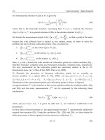
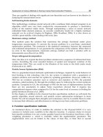
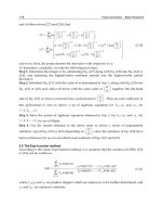
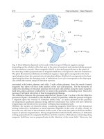
Fig. 7. g -  diagram showing the optimization process of the eigenvalue, 

.


Fig. 8. Eigenstructure of the self-similar solution.

Heat Conduction – Basic Research

290
Under the condition that the right integrated curve is to converge to ==0, each curve
has already optimized with respect to 

as was shown in Fig. 6. Other fixed parameters are
the same as in Fig. 6.
The normalized physical quantities are obtained as a result of the two-dimensional
eigenvalue problem with fixed parameters, =2, =13/2, and =5/3.

5. Conclusions
The crucial role of dimensional analysis and self-similarity are discussed in the introduction
and the three subsequent examples. Self-similar solutions for individual cases have been
demonstrated to be derivable by applying the Lie group analysis to the set of PDE for the
hydrodynamic system, taking nonlinear heat conductivity into account as the decisive
physical ingredient. The scaling laws for thermally conductive fluids are conspicuously
different from those for adiabatic fluids (not discussed in the present chapter; see references
by Murakami et al., 2002, 2005 for details). The former has one freedom less than the latter
due to the additional constraint of thermal conductivity. If a thermo-hydrodynamic system
comprises multiple heat conduction mechanisms, self-similarity cannot be expected in a
vigorous sense except for special cases. However, self-similarity and scaling laws can always
be found at least in an approximate manner, by shedding light on the dominant conduction
mechanism, which should give the basis of system design and diagnostics for scaled
experiments for individual cases. The necessity of dimensional analysis and finding self-
similar solutions is encountered in many problems over wide ranges of research. The simple
general scheme and the examples mentioned in this chapter will help the reader who
encounters a similar situation in his or her investigation find the underlying physics and
prepare further theoretical and experimental setup.
6. References
Antonova, R.N. & Kazhdan, Y.M. (2000). “A self-similar solution for spherically symmetric
gravitational collapse ” Astronomy Letters, Vol. 26, pp. 344 - 355.
Barenblatt, G.I. (1979). Similarity, Self-Similarity, and Intermediate Asymptotics (New York:
Consultants Bureau).
Basko, M.M. & Murakami, M., (1998). “Self-similar implosions and explosions of radiatively
cooling gaseous masses” Phys. Plasma, Vol. 5, pp. 518 – 528.
Bernstein, I.B. ＆ Book, D.L. (1978). “Rayleigh-Taylor instability of a self-similar spherical
expansion” Astrophysical Journal, Vol. 225, pp. 633 – 640.
Gitomer, S.J.; Morse, R.L. & Newberger, B.S. (1977). “Structure and scaling laws of laser-
driven ablative implosions”, Phys. Fluids Vol. 12, pp. 234 - 238.
Guderley, G. (1942) “Starke kugelige und zylindrische Verdichtungsstoße in der Nahe des

Kugelmittelpunktes bzw. der Zylinderachse” Luftfahrtforschung Vol. 19, pp. 302–
312.
Gurevich, A.V.; Parrska, L.V. & Pitaevsk, L.P. (1966). “Self-similar motion of rarefied
plasma” Sov. Phys. JETP, Vol. 22, pp. 449 - &.
Kull, H.J. (1989). “Incompressible Description of Rayleigh-Taylor Instabilities in Laser-
Ablated Plasmas” Phys. Fluids, Vol. B1, pp.170 - 182.
Kull, H.J. (1991). “Theory of Rayleigh-Taylor Instability” Phys. Reports, Vol.206, pp.197 - 325.

Self-Similar Hydrodynamics with Heat Conduction

291
Landau, L.D. & Lifshitz, E.M. (1959). Fluid Mechanics (New York: Pergamon).
Larson, R.B. (1969). ”Numerical calculations of the dynamics of collapsing proto-star” Mon.
Not. R. Astr. Soc., Vol. 145, pp. 271-&.
Lie, S. (1970). Theorie der Transformationsgruppen (New York: Chelsea).
London, R.A. & Rosen, M.D. (1986) “Hydrodynamics of Exploding Foil X-ray Lasers” Phys.
Fluids, Vol. 29, pp. 3813 - 3822.
Mora, P. (2003). “Plasma Expansion into a Vacuum” Phys. Rev. Lett. Vol.90, 185002 (pp. 1 -
4).
Murakami, M.; Meyer-ter-Vehn, J. & Ramis, R. (1990). ”Thermal X-ray Emission from Ion-
Beam-Heated Matter” J. X-ray Sci. Technol., Vol. 2, pp. 127 - 148.
Murakami, M. & Meyer-ter-Vehn, J. (1991) “Indirectly Driven Targets for Inertial
Confinement Fusion” Nucl. Fusion, Vol. 31, pp. 1315 – 1331.
Murakami, M., Shimoide, M., and Nishihara, K. (1995). “Dynamics and stability of a
stagnating hot spot” Phys. Plasmas, Vol.2, pp. 3466 - 3472.
Murakami, M. & Iida, S., (2002). “Scaling laws for hydrodynamically similar implosions
with heat conduction”, Phys. Plasmas, Vol.9, pp.2745 - 2753.
Murakami, M.; Nishihara, K. & Hanawa, T. (2004). “Self-similar Gravitational Collapse of
Radiatively Cooling Spheres”, Astrophysical Journal, Vol. 607, pp.879 - 889.
Murakami, M.; Kang, Y G.; Nishihara, K.; Fujioka, S. & Nishimura, H. (2005). “Ion energy

spectrum of expanding laser-plasma with limited mass”, Phys. Plasmas, Vol.12, pp.
062706 (1-8).
Murakami, M. & M. M. Basko (2006). “Self-similar expansion of finite-size non-quasi-neutral
plasmas into vacuum: Relation to the problem of ion acceleration”, Phys. Plasmas,
Vol. 13, pp. 012105 (1-7).
Murakami, M.; Fujioka, S.; Nishimura, H.; Ando, T.; Ueda, N.; Shimada, Y. & Yamaura, M.
(2006). “Conversion efficiency of extreme ultraviolet radiation in laser-produced
plasmas”, Phys. Plasmas, Vol.13, pp. 033107 (1-8).
Murakami, M.; Sakaiya, T. & Sanz, J. (2007). “Self-similar ablative flow of nonstationary
accelerating foil due to nonlinear heat conduction”, Phys. Plasmas, Vol. 14, pp.
022707 (1-7).
Pakula, R. & Sigel, R., (1985). “Self-similar expansion of dense matter due to heat-transfer by
nonlinear conduction ” Phys. Fluids, Vol. 28, pp. 232 - 244.
Penston, M.V. (1969). “Dynamics of Self-Gravitating Gaseous Spheres – III Analytical
Results in the Free-Fall of Isothermal Cases” Mon. Not. R. astr. Soc., Vol. 144, pp. 425
- 448.
Sedov, L.I. (1959). Similarity and Dimentional Methods in Mechanichs (New York : Academic).
Sanz, J.; Nicolás, J.A.; Sanmartín, J.R. & Hilario, J. (1988). “Nonuniform target illumination in
the deflagration regime: Thermal smoothing”, Phys. Fluids, Vol. 31, pp. 2320 – 2326.
Takabe, H; Montierth, L. & Morse, R.L. (1983). ”Self-consistent Eigenvalue Analysis of
Raileigh-Taylor Instability in an Ablating Plasma”, Phys. Fluids, Vol. 26, pp. 2299 -
2307.
True, M.A.; Albritton, J.R. & Williams, E.A. (1981). “Fast Ion Production by Suprathermal
Electrons in Laser Fusion Plasmas”, Phys. Fluids Vol. 24, pp. 1885 - 1893.

Heat Conduction – Basic Research

292
Zel'dovich, Ya.B. & Raizer, Yu.P. (1966). Physics of Shock Waves and High Temperature
Hydrodynamic Phenomena (New York: Academic Press).

Part 4
Numerical Methods

13
Particle Transport Monte Carlo Method
for Heat Conduction Problems
Nam Zin Cho
Korea Advanced Institute of Science and Technology (KAIST), Daejeon,
South Korea
1. Introduction
Heat conduction [1] is usually modeled as a diffusion process embodied in heat conduction
equation. The traditional numerical methods [2, 3] for heat conduction problems such as the
finite difference or finite element are well developed. However, these methods are based on
discretized mesh systems, thus they are inherently limited in the geometry treatment. This
chapter describes the Monte Carlo method that is based on particle transport simulation to
solve heat conduction problems. The Monte Carlo method is “meshless” and thus can treat
problems with very complicated geometries.
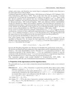
The method is applied to a pebble fuel to be used in very high temperature gas-cooled
reactors (VHTGRs) [4], which is a next-generation nuclear reactor being developed.
Typically, a single pebble contains ~10,000 particle fuels randomly dispersed in graphite–
matrix. Each particle fuel is in turn comprised of a fuel kernel and four layers of coatings.
Furthermore, a typical reactor would house several tens of thousands of pebbles in the core
depending on the power rating of the reactor. See Fig. 1. Such a level of geometric
complexity and material heterogeneity defies the conventional mesh–based computational
methods for heat conduction analysis.
Among transport methods, the Monte Carlo method, that is based on stochastic particle
simulation, is widely used in neutron and radiation particle transport problems such as
nuclear reactor design. The Monte Carlo method described in this chapter is based on the
observation that heat conduction is a diffusion process whose governing equation is analogous
to the neutron diffusion equation [5] under no absorption, no fission and one speed condition,

which is a special form of the particle transport equation. While neutron diffusion
approximates the neutron transport phenomena, conversely it is applicable to solve diffusion
problems by transport methods under certain conditions. Based on this idea, a new Monte
Carlo method has been recently developed [6-8] to solve heat conduction problems. The
method employs the MCNP code [9] as a major computational engine. MCNP is a widely used
Monte Carlo particle transport code with versatile geometrical capabilities.
Monte Carlo techniques for heat conduction have been reported [10-13] in the past. But most of
the earlier Monte Carlo methods for heat conduction are based on discretized mesh systems,
thus they are limited in the capabilities of geometry treatment. Fraley et al[13] uses a
“meshless” system like the method in this chapter but does not give proper treatment to the
boundary conditions, nor considers the “diffusion-transport theory correspondence” to be
described in Section 2.2 in this chapter. Thus, the method in this chapter is a transport theory
treatment of the heat conduction equation with a methodical boundary correction. The

Heat Conduction – Basic Research

296
transport theory treatment can easily incorporate anisotropic conduction, if necessary, in a
future study.


(c) A pebble-bed reactor core
(a) A pebble fuel element
(b) A coated fuel particle
Fig. 1. Cross-sectional view of a pebble fuel (a) consisting several thousands of coated fuel
particles (b) in a reactor core (c)
2. Description of method
2.1 Neutron transport and diffusion equations
The transport equation that governs the neutron behavior in a medium with total cross
section

(, )

t
rE
and differential scattering cross section
(, , )






s
rE E
is given as [5]:

ts
(r,E, ) (r,E) (r,E, ) dE d (r,E E, ) (r,E , )
S(r ,E, )
      


  
    







  


(1a)
with boundary condition, for n,


 0




s
s
(E, ), given,
(r ,E, )
, if vacuum,








0



(1b)

Particle Transport Monte Carlo Method for Heat Conduction Problems

297
where
r neutron position,
E neutron energy,
neutron direction,
Sneutron source,
(r ,E, ) neutron angular flux.














Fig. 2. Angular flux and boundary condition
Fig. 2 depicts the meaning of angular flux (r,E, )





and boundary condition. In the
special case of no absorption, isotropic scattering, and mono-energy of neutrons, Eq. (1)
becomes

   


   
1
44
ss
S(r )
(r, ) (r) (r, ) (r) (r) ,




 
(2a)
with vacuum boundary condition,

s
(r , )
f
or n ,
 

00





(2b)
where scalar flux is defined as
(r) d (r, ).

 






(2c)
Let us now consider a “scaled” equation of (2a),

   


   
11
44
ss
S(r )
(r, ) (r) (r, ) (r) (r) .




 

(3)
An important result of the asymptotic theory provides correspondence between the
transport equation and the diffusion equation, i.e., the asymptotic
()


solution of Eq. (3)
satisfies the following diffusion equation:

Heat Conduction – Basic Research

298

s
(r) S(r),
(r)



1
3



(4a)
with vacuum boundary condition

s
(r d) , d extrapolation distance.



0

(4b)
It is known that, between the two solutions from transport theory and from diffusion
theory, a discrepancy appears near the boundary. Thus, the problem domain is extended
using an extrapolated thickness (typically
t
d one mean free path /


1

) for boundary layer
correction, as shown in Fig. 3.



Fig. 3. Boundary correction with an extrapolated layer
2.2 Monte Carlo method for heat conduction equation
Correspondence
The steady state heat conduction equation for a stationary and isotropic solid is given by [1]:

k(r) T(r) q (r) ,



  0



(5a)
with boundary condition

s
T(r ) , 0

(5b)
where
k(r )

is the thermal conductivity and
q(r)



is the internal heat source.
If we compare Eq. (5) with Eq. (4), it is easily ascertained that Eq. (4) becomes Eq. (5) by
setting

Particle Transport Monte Carlo Method for Heat Conduction Problems

299

s
(r) ,
k(r )


1
3



(6)
and

Sq(r),




(7)
with a large

and the problem domain extended by d .
The Monte Carlo method is extremely versatile in solving Eqs. (1), (2) and (3) with very
complicated geometry and strong heterogeneity of the medium. Thus, Eq. (3) is solved by
the Monte Carlo method (with a large

) to obtain (r)


. The result of (r)


is then translated
to provide
s
T(r ) (r ) (r )






as the solution of Eq. (5) [See Fig. 3.]
Here,

 1 is a scaling factor rendering the transport phenomena diffusion-like. A large
scaling factor plays an additional role of reducing the extrapolation distance to the order of a
mean free path. To choose a proper value for

, we introduce an adjoint problem to perform
sensitivity studies, specific results for a pebble problem provided later in this section.
Proof of principles of the method
In order to confirm or provide proof of principles of the Monte Carlo method described in
Section 2.2, first we consider a simple heat conduction problem which allows analytic
solution. The problem consists of one-dimensional slab geometry, isotropic solid, and
uniformly distributed internal heat source under steady state. The left side has reflective
boundary condition and the right side has zero temperature boundary condition. Fig. 4(a)
shows the original problem and Fig. 4(b) shows the extended problem to be solved by the
Monte Carlo method, incorporating the boundary layer correction. Table 1 provides the
calculational conditions.


Fig. 4. A one-dimensional slab test problem

Thermal
Conductivity
( W/cm K )
Internal Heat
Source( W/cm

3
)
Extrapolation Thickness
(
mfp
)
Scaling
Factor
0.5 0.01 1 1
Table 1. Calculation Conditions for Simple Problem
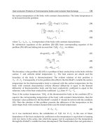
Figs. 5 and 6 show the Monte Carlo method results with and without the extension by
extrapolation thickness in comparison with the analytic solution. Note that the result of the
Monte Carlo method with boundary layer correction is in excellent agreement with the
analytic solution.

Heat Conduction – Basic Research

300




Fig. 5. Monte Carlo heat conduction solution with extrapolated layer



Fig. 6. Monte Carlo heat conduction solution without extrapolated layer
To test the method on a realistic problem, the FLS (Fine Lattice Stochastic) model and
CLCS (Coarse Lattice with Centered Sphere) model [14] for the random distribution of
fuel particles in a pebble are used to obtain the heat conduction solution by the Monte

Carlo method. Details of this process are described in Table 2 and Fig. 7. The power
distribution generated in a pebble is assumed uniform within a kernel and across the
particle fuels. The pebble is surrounded by helium at 1173K with the convective heat
transfer coefficient h=0.1006( W/cm K


2
). A Monte Carlo program HEATON [15] was
written to solve heat conduction problems using the MCNP5 code as the major
computational engine.

Particle Transport Monte Carlo Method for Heat Conduction Problems

301
Material Kernel Buffer Inner PyC SiC
Thermal Conductivity
(
/

WcmK)
0.0346 0.0100 0.0400 0.1830
Radius
(
cm )
0.02510 0.03425 0.03824 0.04177
Material Outer PyC Graphite-matrix Graphite-shell
Thermal Conductivity
(
/


WcmK)
0.0400 0.2500 0.2500
Radius
(
cm
)
0.04576 2.5000 3.0000
Number of Triso Particles 9394
Power/pebble
(
W )
1893.95
Table 2. Problem Description for a Pebble


Fig. 7. A planar view of a particle random distribution for a pebble problem with the FLS
model
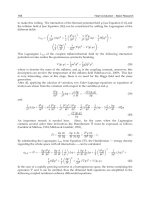
Heat conduction solutions for the pebble problem with the data in Table 2 using the Monte
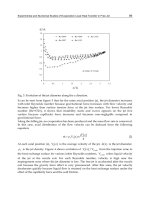
Carlo method are shown in Table 3 and Fig. 8. The number of histories used was
7
10 .
Parallel computation with 60 CPUs (3.2GHz) was used. When the scaling factor

increases,
the solution of the pebble problem approaches its asymptotic solution (diffusion solution).
However, the computational time increases rapidly as the scaling factor increases. In Table 3
and Fig. 8, it is shown that a scaling factor of 10 or 20 is not large enough.

Heat Conduction – Basic Research

302
Scaling
Factor
Maximum
Temp.
(

K
)
Relative
Error
a
(%)
Graphite
Temp. Near
Center(

K
)
Relative
Error
a
(%)
Computing
Time
(sec)
Translation
Temp.
(


K
)
1 1674.21 1.59 158.33 0.71 534 27.08
10 1556.96 1.14 1533.53 0.34 6,692 2.72
20 1558.54 1.12 1531.67 0.30 20,297 1.36
50 1553.22 1.11 1527.07 0.28 99,454 0.54
a
One standard deviation in temperature / mean estimate of temperature by Monte Carlo %100
Table 3. Results of Fig. 7 Problem


Fig. 8. Results along the red line of Fig. 7 vs the scaling factor
Therefore, it is necessary to determine an effective scaling factor that renders the problem
more diffusive. This can be done using an adjoint calculation. Using an adjoint calculation,
the computing time is reduced as the calculation transports particles backward from the
detector region (at the center of the pebble) to the source region. Additionally, it is possible
that the changed tally regions used in the adjoint calculation allow effective particle tallies.

Scaling Factor
Maximum Temp.
(

K
)
Standard
Deviation( 
K
)
Computing Time
(sec)

1 1685.131 0.409 47
20 1558.817 0.308 1,427
50 1553.931 0.304 7,298
80 1553.586 0.304 17,976
100 1552.995 0.303 27,240
120 1552.713 0.303 39,435
Table 4. Maximum Temperature and Computing Time for Fig. 9

Particle Transport Monte Carlo Method for Heat Conduction Problems

303
In order to confirm the appropriate scaling factor, the problem with the data of Table 2 and
in Fig. 7 was again tested with a smaller number (
6
10
) of histories compared to the number
used in the forward calculation. The results depending on the scaling factor are shown in
Fig. 9 and Table 4.
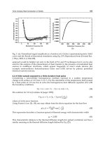
Fig. 9 shows that the center temperature of a fuel pebble approaches its asymptotic solution
(diffusion solution) as the scaling factor increases. Therefore, to obtain a diffusion solution, a
scaling factor of > 30 (e.g., 50) is required.



Fig. 9. Center temperature by the adjoint calculation
2.3 Heat conduction problems
Given varying-temperature boundary condition
The first kind of the boundary conditions is the prescribed surface temperature:

ss

T(r) f(r),



(8)
where
s
r

is on a boundary surface. Since the paradigm heat conduction problem that the
Monte Carlo method can treat is a problem with zero temperature boundary condition (as
described in Section 2.2), let
T be decomposed into
*
T and T

as follows:

*
T(r) T (r) T(r),



(9)
where
*
T
satisfies the zero boundary condition, and T

is chosen such that it satisfies the

given boundary condition (8). Eq. (5a) can then be rewritten as:

*
k(r) T(r) k(r) (T T)
q
(r),


       

 

(10)

Heat Conduction – Basic Research

304
or

**
k(r) T (r)
q
(r),


   


(11a)
where the new source

*
()


qr

is defined by

*
q
(r) k(r) T(r)
q
(r),



  

 

(11b)
Eq. (11a) is to be solved for
*
T
by the Monte Carlo method [6-8]. The Monte Carlo method
cannot deal easily with the gradient term,
()

kr T



, in Eq. (11b) when the boundary
condition temperature is not a constant and
k(r )

is not smooth enough. In order to evaluate
the new source term as simply as possible, let
T

be zero in internally complicated thermal
conductivity region as shown in Fig. 10. In addition,
T

and T


must be continuous in the
whole problem domain to render the
k(r ) T




term treatable.

Fig. 10. Solution Decomposition
*
TT T,





Particle Transport Monte Carlo Method for Heat Conduction Problems

305
In Ref. [8], the followingT

is chosen for a three-dimensional spherical model:

s
s
(r r )
TU(r)f(r,,) ,
(r r )




2

0
2
0

(12)
where
s
f(r , , )


is the given boundary condition (8),

and

indicate polar and azimuthal
angle, respectively.
s
r is radius to the boundary surface and there may be internally
complicated thermal conductivity region inside
r
0
.
Convection boundary condition
A convection boundary condition is usually given by

s
bs
T(r )
k h(T T(r )),
n




1


(13)
where
1
k is the thermal conductivity of medium 1 (solid),
h
and
b
T are the convective heat
transfer coefficient and the bulk temperature of the convective medium, respectively. This
condition can be equivalently transformed to a given temperature
()
b
T boundary condition
of a related problem, in which the convective medium is replaced by a hypothetical
conduction medium with thermal conductivity

s
b
r
khn ,
r





2
(14)
where
n is additional thickness beyond
sbs
r( n r r)  in a spherical geometry. Here
b
r is
the radius where
b
T occurs.
2
k involves a geometry factor and
2
k ’s for several geometries are
shown in Table 5 (see Appendix B for the derivation).

Geometry
2
k
Sphere
s
bs
b
r
h(r r )
r






Cylinder
b
s
s
r
hr ln
r




Slab
bs
h(x x )

Table 5.
2
k for Several Geometries
There is no approximation in the
2
k expressions for given h if there is no heat source in the
fluid. The transformed problem can then be solved by the Monte Carlo method in Section
2.1 with replacement of
0
r by
s
r and

s
r by
b
r , and
b
T as the boundary condition. Eq. (13)
with the right-hand side replaced by Eq. (14) is no more than a continuity expression of heat
flux on the interface. Fig. 11 shows the concept in this transformation.

Heat Conduction – Basic Research

306




(a) Original problem




(b) Equivalent problem


Fig. 11. Transformation of a convective medium to an equivalent conduction medium
preserving heat flux

Particle Transport Monte Carlo Method for Heat Conduction Problems

307

Examples
The method is applied to a pebble fuel with Coarse Lattice with Centered Sphere (CLCS)
distribution of fuel particle [14]. The description of a pebble fuel is shown in Fig. 12 and
Table 2. The pebble fuel is surrounded by helium at given bulk temperature with convective
heat transfer coefficient
2
0.1006( / )

hWcmK. The number of histories used in the
Monte Carlo calculation was
7
10 .




Fig. 12. CLCS distribution
Test Problem 1 is defined by the following non-constant bulk temperature of the helium
coolant:

(cos)K,


1173 10 1
(15a)
where

is the polar angle, or equivalently

z

,
xyz






222
1173 10 1 (15b)
where

b
x
y
zr,
2222
(15c)
with
3.1
b
r , ,
x
y and z in centimeters.
The results are shown in Figs. 13, 14 and 15.

Heat Conduction – Basic Research

308

Fig. 13. Temperature distribution along
x
-direction with 0

yz in Test Problem 1


Fig. 14. Temperature distribution along
z -direction with 0

xy in Test Problem 1

Particle Transport Monte Carlo Method for Heat Conduction Problems

309











Fig. 15. Comparison of Test Problem 1 and a problem with constant helium bulk
temperature (1173

K

)
Test Problem 2 is defined by the following non-constant bulk temperature of the helium
coolant:

(x y z) K

1173 10 (16a)
where

b
x
y
zr,
2222
(16b)
with
3.1
b
r , ,
x
y and z in centimeters.
The results are shown in Figs. 16, 17, and 18.

Heat Conduction – Basic Research

310

Fig. 16. Temperature distribution along
x
-direction with 0


yz in Test Problem 2


Fig. 17. Temperature distribution along
z -direction with 0

xy in Test Problem 2

Particle Transport Monte Carlo Method for Heat Conduction Problems

311

Fig. 18. Temperature distribution along
y -direction with 0

xz in Test Problem 2
3. Applications
3.1 Comparison between the FLS (Fine Lattice Stochastic) model and analytic bound
solutions
In this section, the data of the geometry information and thermal conductivity are identical
to those in Table 2. Based on the results in the previous section, temperature distributions
were calculated using a scaling factor of 50. Three triso particle configurations obtained by
randomly distributed fuels in a pebble were considered (using the FLS model in Ref. 14).
The tally regions as shown in Fig. 19 were chosen. If a (fine) lattice has a heat source, the
tally is done over the kernel volume. If the lattice consists of only graphite, tally is done over
the lattice cubical volume.


Fig. 19. Tally regions with and without a heat source

Heat Conduction – Basic Research

312
Fig. 20 shows the temperature distributions obtained from the Monte Carlo method
compared to the two analytic bound solutions superimposed with a particle located at the
center of the pebble based on commonly quoted homogenized models [16]. It is important to
note that the volumetric analytic solution usually presented in the literature [17] predicts
lower temperatures than those of
(thus underestimates) the Monte Carlo results. In the Monte Carlo results, the fuel-kernel
temperature and graphite-matrix temperature are distinctly calculated. The results are
summarized in Table 6.


Fig. 20. Temperature profiles depending on the triso particle distribution configuration
compared to two homogenized models


Max. Temp.
(
K
)
Average Kernel Temp.
(
K
)
Average Graphite Temp.
(
K
)

Case 1 1555.07 1497.84 1487.61
Case 2 1553.77 1499.63 1480.43
Case 3 1550.87 1501.89 1489.38
Average 1553.23 1499.79 1485.80
Table 6. Maximum, Average Kernel and Graphite Temperatures from Fig. 20
For a fourth triso particle configuration (Case 4), the tally region was further refined as
shown in Fig. 21 to provide more accurate graphite-moderator temperature. Essentially, if
the lattice has a kernel (heat source), the tally is done over the kernel volume and over the
moderator (graphite and layers) volume separately. Otherwise, if the lattice consists of only
graphite, the tally is done over the cubical volume.

Particle Transport Monte Carlo Method for Heat Conduction Problems

313






Fig. 21. Tally regions depending on the geometries
In this problem, geometry information is identical to those shown in Table 2. The distributed
particle configuration is shown in Fig. 22. The kernel and graphite-moderator temperatures
are shown in Fig. 23 and Table 7.

Fig. 22. A planar view of a fourth particle distribution configuration with the FLS model