Developments in Heat Transfer Part 2 pdf

Heat Transfer for NDE: Landmine Detection 9
solution of the heat equation and the use of inverse problems techniques, López (2003); López
et al. (2009; 2004). The process starts with the acquisition of a sequence of infrared images
of the surface of the soil under known heating and atmospheric conditions. As explained
before, sunrise and sunset are the preferred times for detection. We will also assume that
a pre-processing stage is run on a conventional PC in order to align the images and map
grayscale colors to temperature values on the surface. Next, the soil inspection procedure
itself starts. First, we run a detection procedure, as will be explained in the following section,
to obtain the mask of potential targets. Then, a quasi-inverse process operator is used to
identify the presence of antipersonnel mines among the potential targets. For those targets
that failed to be classified as mines (and are therefore labeled as unknown), a full inverse
procedure to extract their thermal diffusivity will be run in order to gain information about
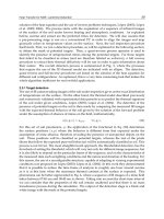
their nature. The overall detection process is summarized in Fig. 3, where the processes
that require the use of the 3D thermal model are indicated with an ellipse. The detection,
quasi-inverse and full-inverse procedures are based on the solution of the heat equation for
different soil configurations. As explained, this is a very time consuming task that makes the
whole algorithm inefficient for real on-field applications.
2.3.1 Target detection
The use of IR cameras taking images of the soil under inspection gives us the exact distribution
of temperatures on the surface. On the other hand, the thermal model described previously
and extensively validated with experimental data permits us to predict the thermal signature
of the soil under given conditions, López (2003); López et al. (2004). The detection of the
presence of potential targets on the soil is then made by comparing the measured IR images
with the expected thermal behavior of the soil given by the solution of the forward problem
under the assumption of absence of mines on the field, mathematically,
α
(x, y, z)=α
soil
, ∀x, y, z. (21)
For this set of soil parameters, p, the application of the functional in Eq. (20) determines
the surface positions

(x, y) where the behavior is different from that expected under the
assumption of mine absence, therefore revealing the presence of unexpected objects on the
soil. These positions will be classified as potential targets, whereas the rest of the pixels
(those that follow the expected pure-soil behavior) will be automatically classified as soil. This
process is not trivial. The most straightforward approach, the thresholded detection, has the
drawback of setting the threshold, which will vary not only for different image sequences, but
it is also likely to depend on the particular frame of the sequence, and on the characteristics of
the measured data such as lighting conditions and the nature and duration of the heating. For
this reason, the use of a reconfigurable structure, capable of adapting to varying experimental
conditions was proposed on López (2003); López et al. (2004). In this work they demonstrated
that it is possible to reduce the time frame of analysis to roughly one hour around sunrise
as it is at this time when the maximum thermal contrast at the surface is expected. This
phenomena can be better appreciated in Fig. 4, where a sequence of IR images of a mine field
taken between 07:40 am and 08:40 am is shown. Taking into account the short time interval
we can consider that the properties of the soil remain unaltered and that there is no mass
transference process during the simulation. The output of the detection stage is a black and
white image with the mask of the potential targets.
29
Heat Transfer for NDE: Landmine Detection
10 Will-be-set-by-IN-TECH
Fig. 3. Structure of the approach used to detect buried landmines using infrared
thermography.
(a) 7:40 am (b) 08:00 am (c) 08:30 am (d) 09:00 am
Fig. 4. Measured IR images of a minefield at sunrise.
2.3.2 Quasi-inverse operator for the classification of the detected targets
In the previous section we dealt with the identification of the (x, y) position of the potential
targets on the soil. In this section we will propose an operator for their classification
into either mine or soil categories; any target that fails to fit into these categories will be
30
Developments in Heat Transfer

Heat Transfer for NDE: Landmine Detection 11
classified as unknown (a procedure for the retrieval of further information about the nature
of the unknown targets will be explained in the next section). For the mine category, the
depth of burial will be also estimated. In general, this reconstruction is not possible unless
additional information on the solution is incorporated in the model by means of the so-called
regularization techniques Engl et al. (1996); Kirsch (1996). It is, however, possible to solve
the inverse problem without the explicit use of a regularization strategy under proper
initialization conditions and the use of iteration methods.
The iterative procedure is based on evaluating Eq. (20), which expresses the deviation between
the observed IR data, y
δ
, and the one given by the solution of the forward problem using
known parameter distributions, F
[p]. Therefore the heat equation needs to be solved for each
of these distributions during the time of analysis (usually one hour around sunrise). In the
case of mine targets, we will assume that their thermal evolution is driven by the thermal
properties of the explosive used, which is commonly TNT composition B-3 or, less frequently,
Tetryl. Our initial guess will be to assume that, (i) all the targets detected in the detection step
are mines, that is,
α
target
= α
mine
, (22)
and (ii) the possible depths of burial constitute a discrete set z
∈
˜
Z being,
˜
Z

= {k Δz, ∀k = 0, 1, , d}, (23)
with Δz the discretization step and d Δz the a depth of burial at which is satisfied the
deep-ground condition, see Eq. (4). The situation k
= 0 corresponds to surface-laid mines.
These two assumptions imply a reduction of the search space, therefore the quasi-inverse
nature of the classification effort that will either confirm or reject them. Let,
•
{y
δ
s
}, s = 1, , S, be the acquired IR image sequence, being S the total number of frames.
• F
[p]
s,k
, the modeled temperature distribution on the soil surface at time s. F[p]
s,k
is
estimated by considering that all the detected targets are landmines buried at the depth
given by index k in Eq. (23).
Note that, in the following, we will concentrate only on those areas of the image that were
marked as possible targets in the detection phase. The classification map for the detected
targets is obtained through the definition of a classification operator which includes the
following computations:
1. For each time instant s
= 1, , S and burial depth k = 0, , d, an error map, J
s,k
= F[p]
s,k
−
y

δ
s
, is estimated by evaluating Eq. (20) for each pixel position (x, y);
2. For each time instant s, a global error map (J
s
) and a global classification map (Υ
s
)are
estimated iteratively by comparing the error maps J
s,k
, k = 0, , d, as follows:
• Initialization step: For each pixel
(x, y), we set J
s
(x, y)=ε (where ε is a predefined
threshold error value); and Υ
s
(x, y)=soil.
• Iterative update step: For each depth of burial, k, with k
= 0, , d, J
s
(x, y)=
min(J
s,k
(x, y), J
s
(x, y)) and Υ
s
(x, y)=ar g mi n
k

(J
s,k
(x, y), J
s
(x, y)) (the category for
which the error is smaller, i.e. the depth of burial). If J
s
(x, y) > ε then Υ
s
(x, y) is
set to Unknown.
3. Once J
s
and Υ
s
have been obtained, we combine all these partial maps (J
s
, resp. Υ
s
) into
single ones (J, resp. Υ) in the following way:
31
Heat Transfer for NDE: Landmine Detection
12 Will-be-set-by-IN-TECH
• Υ: Pixels classified as mines at any processing step are kept in the final classification
map. For the others, we keep the category that appears more times.
• J
(x, y)=max
s
(J

s
(x, y)). This is a very conservative approach aiming at reducing the
number of false negatives (failure to detect a buried mine) even at the cost of increasing
the false alarm rate of the system.
• To find a trade-off between the accuracy of the classification and the number of false
alarms, we define a cutoff error, e
max
. If the entry on the error map, J for a pixel exceeds
e
max
, the pixel will be automatically assigned to the category of Unknown. e
max
is
estimated empirically, however it could be estimated taking into account the pixels
classified as non-mine based their temperature variance using bootstrap techniques,
Zoubir & Iskander (2004).
2.3.3 Full-inverse procedure for the classification of non-mine targets
In this case, no assumption about the nature of the targets found in the detection phase is
made, although the set of possible depths at which the targets can be placed is still bounded
by Eq. (23). Under these assumptions, Eq. (22) does not hold and α
target
is unknown and could
take any value depending on the nature of the object. For this reason, it is necessary in this
case to use a systematic approach for the minimization of the functional J, which implies the
calculation of the gradient ∂J/∂p.
Let us consider the existence of a buried target in a 3D soil volume, Ω, with an unknown
α
= α(r), r =(x, y, z) ∈ Ω. The thermal experiment is the following: at time t = t
0
, the solid

is subject to a prescribed flux, q
net
(r

, t), on its surface Γ, being Γ the portion of the surface
∂Ω accessible for measurements. We then measure the temperature response θ
(r

, t) at the
boundary r

∈ Γ, during the time interval [ t
0
, t
f
]. We rewrite our 3D forward problem in
Eq. (1) as,
−div{α(r) gradθ} +
∂θ
∂t
= 0, r ∈ Ω (24a)
θ
(r, t = t
0
)=θ
0
, r ∈ Ω (24b)
∂
∂n
θ(r


, t)=q
net
(r

, t) r

∈ Γ, t ∈ [t
0
, t
f
]. (24c)
We look at the reconstruction of α
(r) from the knowledge of the surface response of
temperature, y
δ
= θ(r

, t), to prescribed flux applied on the boundary q
net
(r

, t). We call data
the pair
(
θ(r

, t), q
net
(r


, t)
)
. As mentioned before, this is an ill-posed problem. It is intuitive
that the data parameters
(r

, t) belong to a 3D subset, because r

∈ Γ and t ∈ [t
0
, t
f
]. This is
sufficient enough for the reconstruction of the function α
(r), defined in a 3D volume. Let us
now introduce the model problem as an initial guess p, such that p
(r

)=α(r

) (known data on
the boundary), with the following governing equations and boundary conditions,
−div{p(r) gradu} +
∂u
∂t
= 0 r ∈ Ω (25a)
u
(r, t = t
0

)=u
0
, r ∈ Ω (25b)
∂
∂n
u(r, t)=q
net
(r

, t) r

∈ Γ, t ∈ [t
0
, t
f
]. (25c)
The solution of Eq. (25) is a well-posed problem, as opposed to Eq. (24), and will be denoted
by u
(r, t; p). Our aim will be to control p in such a way that the difference between the model
and the observed data tends to zero. This goal is quantified by an objective function J to be
32
Developments in Heat Transfer
Heat Transfer for NDE: Landmine Detection 13
minimized. The functional to be minimized is the L
2
norm of the misfit between the model
and the observation given by,
J
(u(p)) ≡
1

2

t
f
t
0

Γ
u(r

, t; p) − θ(r

, t)
2
dS dt. (26)
This is a classic optimization problem which implies the calculation of the gradient of the
functional J. To this aim we will make use of the variational method. If we introduce the
notation,
< u, v >
Ω
=

Ω
u(r) v(r) dΩ
< q
net
, v >
Γ
=


Γ
q
net
(r

) v(r

) dS
a
p
< u, v >=

Ω
p gradu gradvdΩ,
then the model problem, Eq. (25), is equivalent to the variational problem,

t
f
t
0
<
∂u
∂t
, v
>
Ω
dt +

t
f

t
0
(a
p
< u, v >) dt −

t
f
t
0
< q
net
, v >
Γ
dt = 0, ∀v (27)
Eq. (27) can be considered as the constraints in the minimization problem, see Eq. (26).
Therefore, we can introduce the Lagrange multiplier λ
(r, t) and define the Lagrangian L as,
L
(u, p, λ) ≡ J(u)+

t
f
t
0
{<
∂u
∂t
, λ
>

Ω
+a
p
< u, λ > − < q
net
, λ >
Γ
} dt. (28)
Note that L
= J if u is the solution of the model problem, Eq. (25), since Eq.(27) holds for
any λ. Thus, the minimum of J under the constraints in Eq. (27) is the stationary point of
the Lagrangian L. Conversely, if δL
= 0 for arbitrary δλ, u and p being held fixed, it follows
necessarily that Eq. (27) holds. We consider,
δL
=
∂L
∂u
δu
+
∂L
∂p
δp, (29)
where,
∂L
∂u
δu ≡

t
f

t
0
(u − θ, ∂u)
Γ
dt +

t
f
t
0
{(δ
∂u
∂t
, λ)
Ω
+ a
p
(δu, λ)} dt (30a)
∂L
∂p
δp ≡

t
f
t
0

Ω
δp gradu gradλ dΩ δμ. (30b)
We can restrict the choice of λ such that

∂L
∂u
δu
= 0. (31)
This condition can be written as,

t
f
t
0
< u − θ, δu >
Γ
dt +

t
f
t
0
{− < δu,
∂λ
∂t
>
Ω
+a
p
< δu, λ >} dt+ < δu, λ >
Ω
|
t
f

t
0
= 0, (32)
33
Heat Transfer for NDE: Landmine Detection
14 Will-be-set-by-IN-TECH
where δu(x,0)=0. The last term of (32) vanishes if we impose,
λ
(r, t ≥ t
f
)=0. (33)
By doing so we obtain the equation for the adjoint field λ,
−div{p gradλ}−
∂λ
∂t
= 0, r ∈ Ω (34a)
λ
(r, t ≥ t
f
)=0, r ∈ Ω (34b)
∂
∂n
λ(r

, t)=θ − u, r ∈ Γ. (34c)
This is the so called back diffusion equation for the adjoint field, and it is also a well posed
problem. With this choice of the adjoint field λ
(r, t), the variation ∂J becomes
∂J
=


t
f
t
0

Ω
∂p gradu gradλ dΩ dt. (35)
It results from Eq. (35) that the derivative of J in the p
(r) direction is known explicitly by
solving two problems, the direct problem for the field u and the adjoint problem for the field
λ. That is, the Z-integral,
∂J
∂p
≡ Z =

t
f
t
0
gradu gradλ dt. (36)
Solving Eq. (25) and Eq. (34), both of them well-posed forward problems, and using Eq. (36),
the expression of the update of Eq. (17)) can be calculated in a straightforward manner. With
respect to the number of iterations of the Landweber method, the selection of the stopping
criteria of the algorithm must be made according to the discrepancy principle in Eq. (18)). The
bigger the η, the lower the number of iterations is, and the higher the error is. The selection
of η for a particular application must then be a trade-off between computational time and
accuracy of the solution.
2.4 Estimation of the computational cost
The algorithm described above is based on iterative procedures involving multiple solutions

of the heat equation for different soil configurations. This constitutes a time consuming
process not feasible for its use on the field as the computational complexity of the FD method,
if N
= n
x
· n
y
· n
z
is the total number of grid nodes, is O(N · IT), where IT is the number
of iterations. As an example, we consider the analysis of a piece of soil (α
soil
= 6.4 · 10
−7
m/s
2
) of moderate dimensions of 1m×1m with a shallowly buried mine (α
mine
= 2.64 · 10
−7
m/s
2
). Even if the depth resolution of IRT is barely 10-15 cm, the depth of analysis must be
set to at least 40-50 cm in order to apply the boundary condition in Eq. (4). Using a uniform
spatial discretization of Δx
= Δy = Δz = 0.8 cm and assuming a temporal discretization step
of Δt
= 6.25 s (F
0
= 0.06), for a typical example the simulation of the behavior of the soil

during one hour using C++ (optimized for speed using O2 flag from Microsoft Visual C++
compiler) on a Intel Core2Duo 2.8GHz takes 30 seconds if single precision arithmetic is used to
represent the temperatures. Taking into account that the proposed inverse procedure requires
the solution of the model for multiple soil configurations, the total computing time assuming
that only 100 iterations are needed (a soft approach) will add up to 50 minutes. As this
jeopardizes its use for field experiments we have developed a hardware implementation of a
34
Developments in Heat Transfer
Heat Transfer for NDE: Landmine Detection 15

  


  


Fig. 5. GPU internal structure and memory hierarchy.
heat equation solver. In Pardo et al. (2009; 2010) we presented an FPGA-based implementation
of such a solver. However, the main drawback of an FPGA implementation is the requirement
of the system in terms of memory. The FPGA has a little amount of distributed memory
and the FPGA’s logic blocks can also be configured to behave like memory, however this is
an inefficient way of FPGA using. Some vendors offer cards where external memory and
FPGA are integrated on the same board, allowing to use the FPGA to deal with processing
issues. However, these are expensive solutions. GPUs offers a structure which perfectly
fits with the proposed problem and they have the advantage of being cheaper than FPGAs.
GPUs are present in all computers and therefore we avoid the necessity of having a dedicated
and expensive hardware to deal with our problem. Moreover, the GPU implementation is
hardware independent, in the sense that it can be used on GPUs from NVIDIA with none or
little changes, depending on GPU’s computing capabilities.
3. GPU thermal model implementation

The system that solves the thermal model using the explicit FD method was implemented
using CUDA language, NVIDIA (2010), and projected in a GPU from NVIDIA. The computing
structure of GPUs makes them a suitable candidate to implement algorithms requiring high
computing power. First we will introduce GPU characteristics and some basics abouts its
programming mode. Then, we will present the proposed GPU implementation that simulates
the thermal behavior of the soil and that speeds the computations up compared to a personnel
computer.
3.1 GPU structure
GPUs are made up of several multiprocessors that can perform parallel processing data, which
makes them suitable for processing in systems where it can be split up in independent portions
and processed independently. The structure of such a GPU can be seen in Fig. 5. The GPU is
made up of several multiprocessors, labeled as MP1 MPN in Fig. 5. Moreover, inside each
multiprocessor there are several cores, labeled as C1 CM in Fig. 5. One important issue of
GPU programming concerns to the use of the different memories available in the GPU, see
Fig. 5. The Global Memory is available to all multiprocessors and cores, whereas the Shared
Memory inside each multiprocessor is only available to the corresponding multiprocessor’s
cores. Additionally, each core has its own and private memory space. One key aspect of
a GPU-based system is the memory data organization and access, as they can impose a
35
Heat Transfer for NDE: Landmine Detection
16 Will-be-set-by-IN-TECH




 



















 



















 




















Fig. 6. Structure of threads hierarchy in a GPU (reprinted from NVIDIA (2010)).
bottleneck in the system performance. The global memory has an access latency two orders
of magnitude higher than the access to the shared memory. Thus, it is important to minimize
the use of global memory and maximize, as far as possible, the use of shared memory because
this will increase the performance of the system.
Once the structure of the GPU has been briefly described we will introduce the basic aspects of

GPU programming required to understand the structure of the proposed system . Functions
in CUDA are called kernels and each kernel can be executed in parallel by several threads
1
,as
contrary to ordinary C/C++ functions that can only be executed by one processor. A kernel
is not executed as a single thread, but it is executed as a block of threads, each of them
processing the same function on different data, following a single-program multiple data
(SPMD) computing model. Each thread inside the block has a 1D, 2D or 3D identifier (ID),
depending on the applications, which distinguishes the concrete thread, to compute elements
from a vector, matrix or volume of data. All the threads of a block are executed on the same
multiprocessor and therefore they must fit within the available resources. This sets a limit
on the maximum threads per block, which is limited to 512 in current GPUs. To avoid this
limitation a kernel can be executed in several blocks of threads, which are organized as 1D or
2D groups of threads. The only requirement concerning the block of threads is that they must
1
The thread is the basic element of processing
36
Developments in Heat Transfer
Heat Transfer for NDE: Landmine Detection 17
CUDA cores 128
CUDA Multiprocessors 8
Graphics Clock 738 MHz
Processor Clock 1836 MHz
Global Memory 512 MB
Memory Clock 1100 MHz
Memory Bandwidth 70.4 GB/s
Table 1. GTS 250 NVIDIA GPU main characteristics.














Fig. 7. Temperatures updating scheme on the GPU.
be independent from each other. Fig. 6 shows threads’ hierarchy and its organization in the
GPU.
3.2 GPU implementation of heat equation solver
GPU’s structure fits perfectly our problem, where the full data can be split up in independent
blocks that can be process the data in parallel. Each multiprocessor can work with a portion
of grid’s nodes increasing the performance of the system. The GPU used in this work was a
GTS-250 from NVIDIA (cost around 250e- 300 $), whose characteristics are summarized in
Table 1.
As was pointed, one of the main important aspects in an efficient CUDA-based system is the
correct management of the memory to reduce the access to the global memory. To this aim the
full grid of points, see Fig. 2(a), was divided into volume slices of size size_blockx
× size_blocky,
where the nodes’ temperature of each slice is computed in a block of threads, see Fig. 7. Each
thread of the block is responsible for updating the temperature of the nodes with the same
(x,y) coordinates within the considered piece of soil. The threads advance as a wavefront,
updating the nodes’ temperature starting from the superficial layers to the inside of the soil,
see Fig 7. It can be noted that there are overlapping areas between different blocks of threads,
labeled as boundary nodes and indicated in grey in Fig. 7, which must be taking into account to
compute only once the new temperature value.

Concerning the memory usage, the initial temperatures are stored in the global memory, and
they have been transferred from the HOST memory to GPU global memory prior to the
computation of the new temperatures. The temperatures are duplicated in the memory, as
during one iteration we need to use one location to read temperatures and the other to write
37
Heat Transfer for NDE: Landmine Detection
18 Will-be-set-by-IN-TECH















 


Fig. 8. Data memory transferences during the updating process.
the updated values and in the following iteration the roles are interchanged. The remainder
constant values needed in the computations, such as F
0
and values related to the boundary

conditions, see Eq. (14), are also stored in the global memory. The access to the global memory
should be minimized to increase the speed of the computations, because the global memory
has a high latency access. Thus, we use, during the updating process, the shared memory of
the multiprocessors to accelerate the access to the data. The memory operations are shown in
Fig. 8 where we can see the data transferences between the different memories of the GPU.
In Fig. 8 we will consider the temperature updating process from nodes in Layer K.InSTEP
1 the temperatures of Layer K-1 nodes are stored in both the multiprocessor’s shared memory
and in the cores’ local memory. Moreover, nodes’ temperatures from Layer k are read from the
global memory and stored in the local cores’ memory . During STEP 2 the nodes’ temperatures
from Layer K replace those from Layer K-1 in the shared memory, at the same time, the nodes’
temperatures from Layer K+1 are read from global memory and stored in cores’ local memory.
In STEP 3 all data required to perform Layer K nodes’ temperature updating is available on
the local memory and shared memory. The same temperature of a Layer K is required to
update the temperature of several nodes (the node itself and its north, south, west and east
neighbors). If all nodes had to access global memory to read these values the process would
be slowed, however once they are read from cores’ local memory they are transferred to the
shared memory, where they are available to all threads of the block, thus reducing the time
access to the data. Once a thread has updated the temperature of a node, it uploads to the
main memory the updated value and it continues computing the following temperature node
updating. There is a synchronization process when a thread finishes one node’s temperature
updating because we must ensure that prior to continue with a node of the following layer all
threads have finished the temperatures updating of the current layer.
4. Results
In this section we will introduce the results of the complete system. We divide this section
into two main topics. On the one hand the results of the detection algorithm are shown for
a scenario from the TNO Physics and Electronics Laboratory, Jong et al. (1999). On the other
hand, we will show the performance of the GPU implementation and how it improves the
usability of the detection system reducing the processing time.
4.1 Landmine detection algorithm
Next, we will show the result of the previously described detection algorithm to images

acquired in a real test field. The scenario considered corresponds to the sand lane of the
38
Developments in Heat Transfer
Heat Transfer for NDE: Landmine Detection 19















































Fig. 9. Ground truth of the test field used during the experiment corresponding to a sand
lane with different types of surrogated mines and non-mine targets.
Symbol Category Total
• Surface mine 14
◦ Mine at 1 cm 9
 Mine at 6 cm 9
⊕ Mine at 10cm 1
 Mine at 15cm 1
 Undefined test object 5
 Shell marker 4

Table 2. Symbols used to represent the different categories of targets present in the test field
in Fig. 9.
test facilities of the TNO Physics and Electronics Laboratory. For the experimental setup
considered, the measured thermal diffusivity of the soil was α
sand
= 6 × 10
−7
m
2
/s. With
respect to the test mine targets present, they are surrogated mines and most of them have been
built at TNO-FEL. In all test mines the same substitute for the explosive has been used, RTV,
having the same relevant properties as the real explosive and particularly α
RTV
= 1.13 × 10
−7
m
2
/s. Fig. 9 shows a sample image of the sand lane acquired with the IR sensor and the
position of the different targets considered. Table 2 summarizes the symbols used for
the different categories of targets present. The total number of targets is 43, 34 of which
correspond to landmines. The remaining nine targets are five undefined test objects and four
shells used as markers. We will concentrate on the results of the quasi-inverse and full-inverse
procedures for the classification of mines and non-mine targets respectively.
39
Heat Transfer for NDE: Landmine Detection
20 Will-be-set-by-IN-TECH
Location Detected and classified Total
Surface 12 12
Buried at 1 cm 6 6

Buried at 6 cm 5 6
Buried at 10 cm 1 1
Buried at 15 cm 0 1
Table 3. Summary of the mines correctly detected and classified after the application of the
quasi-inverse operator.
4.1.1 Results of the quasi-inverse operator for the classification of mine targets
The quasi-inverse operator classifies the detected targets as Mine or Unknown. Moreover,
for the Mine class, sub-categories corresponding to their depth of burial are produced. For
the experimental setup in Fig. 9, the results of the application of the quasi-inverse operator
are summarized in Table 3, showing the distribution of mine targets correctly detected and
classified according to their depth of burial with e
max
= 2.6. As can be seen, all the mine
targets on the surface or at 1cm depth were correctly detected and classified, and so were five
out of six of the mines buried at 6 cm. The results for depths of 10 and 15 cm are not conclusive
since only one of each is present, but a degraded performance of the quasi-inverse operator
with depth is to be expected.
The performance of the classification operator is evaluated by making use of two properties,
sensitivity and specificity, Hanley & McNeil (1982),
Sensitivity
=
TP
TP + FN
Specificity
=
TN
TN + FP
(37)
being TP the number of true positives, TN the number of true negatives, FP the number of
false positives and FN the number of false negatives. The performance depends strongly on

the election of e
max
, being a trade-off between sensitivity and specificity, i.e. , between the
number of mine targets correctly classified and the number of false alarms. In humanitarian
operations, the stress is put on the correct location of mines, while reducing the number
of false alarms, although highly desirable, is a secondary goal. With respect to the global
performance, it is clearly a function of the particular value of e
max
. For e
max
= 2.6 we find
that 24 mines were correctly detected and classified over a total of 26.At the same time, the
number of false positives is 13 compared to the 27 after the application of the detection stage
alone.
4.1.2 Results of the full-inverse approach for the classification of non-mine targets
Now, we will illustrate the process of estimating the thermal parameters of non-mine targets
making use of the full inverse process previously described. To this aim, we will consider the
test object V82 present on the minefield (see Fig. 9). This target was classified as unknown by
the quasi-inverse operator and we now aim to infer what type of object it is by estimating its
thermal properties. If we estimate the measurement error to be δ
= 0.3
◦
C and setting η = 0.2,
we have,
μ
> 2
1
+ η
1 − 2η
= 4. (38)

40
Developments in Heat Transfer
Heat Transfer for NDE: Landmine Detection 21
0 50 100 150 200 250
1
2
3
4
5
6
7
Number of Iterations
Error
0 50 100 150 200 250
0
0.2
0.4
0.6
0.8
1
1.2
1.4
1.6
1.8
x 10
−5
Number of iterations
α (m
2
/s)

(a) (b)
Fig. 10. Test target V82: (a) Evolution of the error in the estimation of α; (b) Evolution of the
value of α during the inverse problem procedure.
For μ
= 4.1, the discrepancy principle determines the stopping rule as,
y
δ
− F[p
δ
k
(δ,y
δ
)
]≤1.23 < y
δ
− F[p
δ
k
],0≤ k ≤ k(δ, y
δ
) (39)
The evolution of the error for the Landweber iteration method is shown in figure 10(a). The
stopping criteria in (39) corresponds to a number of iterations of the algorithm N
it
= 230.
Figure 10(b) shows the evolution of the estimation of the α parameter in this case. The final
result obtained for the non-mine target V82 is,
α
V82
= 170 × 10

−7
m
2
/s.
This value is two orders of magnitude bigger than that of the sand (α
sand
≈ 6 × 10
−7
m
2
/s)
which coincides with typical values of the thermal diffusivity of metallic solids.
4.2 GPU heat equation solver
We will now introduce the results obtained with the GPU implementation in terms of system
throughput. As was pointed in the introduction a NVIDIA GTS 250 GPU, a low-cost GPU,
was used to perform the comparison between a purely CPU implementation ( Core2Duo 2.8
GHz implementation in C++) of the heat equation solver and a GPU implementation. One
of the first issues is to think about the blocks threads’ distribution and partitioning. The full
volume of nodes which form the grid of points must be divided into blocks of threads, each
of which is responsible for the nodes’ temperature updating. The idea can be seen in Fig. 7,
where the volume has been divided into blocks of threads of size size_blockx
×size_blocky which
are sent to the MP of th GPU, in this case a 1D array of blocks is shown for the shake of
clarity. Fig. 11(a) shows the performance of the GPU for various block sizes, where we have
chosen size_blockx = size_blocky, and a volume of 800
×800×50 nodes. The results from these
simulations can be seen in Table 4, where the speedup is compared to a purely CPU simulation
of the full volume. It can be noted that the throughput of the system raises up as the size of
the block is increased. This is due to the fact that when small blocks are used there are a lot
41

Heat Transfer for NDE: Landmine Detection
22 Will-be-set-by-IN-TECH









   


(a) Throughput of GPU heat equation solver for different blocks’ size.









  


 
(b) Throughput of GPU and CPU heat equation solvers
implementations for different volume of simulated points. In

the GPU implementation the block grids’ size was set to 16
×16.
Fig. 11. Performance results comparing GPU and CPU throughputs for different setups.
of such small blocks spread over all MP, and therefore there will be a long cue of pending
blocks to be processed. On the contrary, if the size of the blocks is increased we will have less
blocks and the cue of pending blocks to be processed by the MP will be reduced. There is a
limit, imposed by GPU’s structure, given by the maximum number of threads that a MP can
process (512). It can be seen from Fig. 11(a) and Table 4 that the throughput of the system is
increased one order of magnitude when we go from 2
×2to16×16 blocks of threads. Thus
in the following simulations we will used this block’s size for GPU simulations. Fig. 11(b)
shows the GPU and CPU throughput for different nodes volumes, the data can be seen in
Table 5. It can be noted how the performance of the GPU grows up one order of magnitude
when the size of the volume is increased. This is due to the fact that for small volume of nodes
not all GPU’s resources are being used, whereas for big enough size volumes the inherent
parallelism of the GPU increases the throughput of the system. It is obvious that for very
big volumes the throughput will be low because there will be a cue of pending blocks to be
processed which degrades the throughput of the system (note the reduction of the throughput
for the 1024
×1024×50 volume).
42
Developments in Heat Transfer
Heat Transfer for NDE: Landmine Detection 23
block_dimx × block_dimy GPU throughput (Mpoints/s) GPU time (s) Speedup
2×2 120.0 25.6 3.1
4
×4 336.5 9.1 8.7
8
×8 634.3 4.8 16.7
16

×16 1400.0 2 40
Table 4. GPU throughput for a given volume of points and varying block thread’s
dimensions.
Volume GPU throughput (Mpoints/s) CPU throughput (Mpoint/s) Speedup
32×32×50 332 39.3 8.4
64
×64×50 1289.33 39.3 32.6
256
×256×50 1476.67 39.3 37.0
512
×512×50 1496.02 39.3 39.3
1024
×1024×50 1402.8 39.3 36.7
Table 5. Throughput and CPU and GPU solvers of the heat equation solver for different size
volumes.
5. Conclusions
In this chapter, two inverse procedures for the inspection of soils by non-invasive means with
application in antipersonnel mines detection have been presented. The first quasi-inverse
procedure aims at the detection of surface-laid and shallowly buried mines, giving an
estimation of their depth of burial that will be of critical importance during the removal stage.
In the second approach, a full inverse procedure for the identification of the thermal properties
of other objects present on the soil was presented. Both procedures need the recursive solution
of the heat equation problem for different soil configurations, which constitutes a very time
consuming task on a conventional computer. The efficient solution of the aforementioned
procedures is successfully solved using a heat equation solver accelerator based on the use of
GPUs, obtaining speed-up factors over 40. The speedup obtained with the proposed system
with respect to nowadays computers, together with its low-cost and portability justifies the
implementation as it permits its use on the field during demining operations.
6. References
Bach, P., Toumeur, P. L., Poumarkde, B. & Bretteand, M. (1996). Neutron activation and

analysis, EUREL International Conference Detection of Abandoned Landmines, Vol. 431,
pp. 58–61.
Bejan, A. (1993). Heat Transfer, John Wiley & Sons, Inc.
Cameron, M. & Lawson, R. (1998). To Walk Without Fear: The Global Movement to Ban Landmines,
Toronto: Oxford University Press.
Durbano, J., Ortiz, F., Humphrey, J. R., Curt, P. & Prather, D. (2004). Fpga-based acceleration
of the 3d finite-difference time-domain method, Proceedings of the 12th annual IEEE
symposium on Field-Programmable Custom Computing Machines, pp. 156–163.
43
Heat Transfer for NDE: Landmine Detection
24 Will-be-set-by-IN-TECH
Engl, H. W., Hanke, M. & Neubauer, A. (1996). Regularization of Inverse problems, Kluwer
Academic Publishers.
England, A., Galantowiz, J. & Schretter, M. (1992). The radiobrightness thermal inertia
measure of soil moisture, IEEE Transactions on Geoscience and Remote Sensing
30(1): 132–139.
England, A. W. (1990). Radiobrigthness of diurnally heated, freezing soil, IEEE Transactions on
Geoscience and Remote Sensing 28(4): 464–476.
Englelbeen, A. (1998). Nuclear quadrupole resonance mine detection, CLAWAR’98,
pp. 249–253.
Furuta, K. & Ishikawa, J. (eds) (2009). Anti-personnel landmine detection for humanitarian
demining: the current situation and future direction for Japanese research and development,
Springer-Verlag.
Gros, B. & Bruschini, C. (1998). A survey on sensor technology for landmine detection, Journal
of Humanitarian Demining pp. 172–187.
Hanley, J. & McNeil, B. (1982). The meaning and use of the area under a receiver operating
characteristic (ROC) curve, Radiology 143: 29–36.
Horowitz, P. (1996). New technological approaches to humanitarian demining, Technical Report
JSR-96-115, JASON MITRE.
Hwu, W. W., Keutzer, K. & Mattson, T. (2008). The concurrency challenge, IEEE Design & Test

of Computers 25(4): 312 – 320.
ICBL (2006). Landmine Monitor Report 2006, International campaign to can landmines (ICBL).
Incropera, F. & DeWitt, D. (2004). Introduction to Heat Transfer, 4th edn, John Wiley & Sons.
Jankowski, P., Mercado, A. & Hallowell, S. (1992). FAA explosive vapor/particle detection
technology, Applications of Signal and Image Processing in Explosives Detection Systems,
Vol. 1824, pp. 13–27.
Jong, W., Lensen, H. & Janssen, H. (1999). Sophisticated test facilities to detect land mines,
Detection and Remediation Technologies for Mines and Minelike Targets IV, Vol. 3710 of
Proceedings of the SPIE, pp. 1409–1418.
Kahle, A. B. (1977). A simple thermal model of the earth’s surface for geologic mapping by
remote sensing, Journal of Geophysical Research 82: 1673–1680.
Khanafer, K. & Vafai, K. (2002). Thermal analysis of buried land mines over a diurnal cycle,
IEEE Transactions on Geoscience and Remote Sensing 40(2): 461–473.
Kirsch, A. (1996). An introduction to the Mathematical Theory of Inverse problems, Vol. 120 of
Applied mathematical sciences, Springer-Verlag, New York.
Larsson, C. & Abrahamsson, S. (1993). Radar, multispectral and biosensor techniques for mine
detection, Symposium on Anti-Personnel Mines, pp. 179–202.
Liou, Y. & England, A. (1998). A land surface process/radiobrightness model with couple heat
and moisture transport for freezing soils, IEEE Transactions on Geoscience and Remote
Sensing 36(2): 669–677.
Lockwood, G., Shope, S., Bishop, L., Selph, M. & Jojola, J. (1997). Mine detection using
backscatered x-ray imaging of antitank and antipersonnel mines, Detection and
Remediation Technologies for Mines and Minelike Targets II 3079: 408–417.
López, P. (2003). Detection of Landmines from Measured Infrared Images using Thermal Modeling of
the Soil, PhD thesis, Universidad de Santiago de Compostela.
44
Developments in Heat Transfer
Heat Transfer for NDE: Landmine Detection 25
López, P., Pardo, F., Sahli, H. & Cabello, D. (2009). Non-destructive soil inspection using an
efficient 3d softwareâ

˘
A¸Shardware heat equation solver, Inverse Problems in Science and
Engineering 6(17): 755–775.
López, P., van Kempen, L., Sahli, H. & Cabello, D. (2004). Improved thermal analysis of buried
landmines, IEEE Transactions Geoscience and Remote Sensing 42(9): 1955–1964.
Maksymonko, G. B. & Le, N. (1999). Performance comparison of standoff minefield detection
algorithms using thermal IR image data, Vol. 3710, SPIE, pp. 852–863.
URL: />NVIDIA (2010). NVIDIA CUDA C Programming Guide 3.1, NVIDIA Corporation Technical
Staff.
Ottawa (1997). Convention on the prohibition of the use, stockpiling, production and transfer
of anti-personnel mines and on their destruction.
Pardo, F., López, P., Cabello, D. & Balsi, M. (2009). Effcient software-hardware 3d heat
equation solver with applications on the non-destructive evaluation of minefields,
Computers & Geoscience 35: 2239–2249.
Pardo, F., López, P., Cabello, D. & Balsi, M. (2010). Fpga computation of the 3d heat equation,
Computational Geoscience 14: 649–664.
Placidi, P., Verducci, L., Matrella, G., Roselli, L. & Ciampiolini, P. (2002). A custom VLSI
architecture for the solution of FDTD equations, IEICE Transactions on Electronics
E85-C: 572–577.
Pregowski, P., Walczack, W. & Lamorski, K. (2000). Buried mine and soil temperature
prediction by numerical model, Proceedings of the SPIE, Detection and Remediation
Technologies for Mines and Minelike Targets V, Vol. 4038, pp. 1392–1403.
Robledoa, L., Carrascoa, M. & Merya, D. (2009). A survey of land mine detection technology,
International Journal of Remote Sensing 30(9): 2399–2410.
Sabatier, J. & Xiang, N. (2001). An investigation of a system that uses acoustic seismic coupling
to detect buried anti-tank mines, IEEE Transactions on Geoscience and Remote Sensing
39(6): 1146–1154.
Schneider, R., Turner, L. & Okoniewski, M. (2002). Application of FPGA technology to
accelerate the Finite-Difference Time-Domain (FD-TD) method, Proceedings of the 10th
ACM/SIGDA International Symposium on Field-Programmable Gate Arrays, pp. 97–105.

Siegel, R. (2002). Land mine detection, IEEE Instrumentation & Measurement Magazine
pp. 22–28.
Thanh, N., Hao, D. N. & Sahli, H. (2009). Augmented Vision Perception in Infrared Algorithms
and Applied Systems, Advances in Pattern Recognitiob, SpringerLink, chapter Infrared
Thermography for Land Mine Detection, p. 471.
Thanh, N., Sahli, H. & Hao, D. (2007). Finite-Difference methods and validity of a thermal
model for landmine detection with soil propierty estimation, IEEE Transactions on
Geoscience and Remote Sensing (4): 656–674.
Thanh, N., Sahli, H. & Hao, D. (2008). Infrared thermography for buried landmine
detection: inverse problem settin, IEEE Transactions on Geoscience and Remote Sensing
(12): 3987–4004.
Vines, A. & Thompson, H. (1999). Thompson, beyond the landmine ban: Eradicating a lethal
legacy, Technical report, Research Institute for the Study of Conflict and Terrorism.
45
Heat Transfer for NDE: Landmine Detection
26 Will-be-set-by-IN-TECH
Wang, T. & Chen, C. (2002). 3-D thermal-ADI: A linear-time chip level transient thermal
simulator, IEEE Transactions on Computer-Aided Design of Integrated Circuits and
Systems 21(12): 1434–1445.
Zoubir, A. M. & Iskander, R. (2004). Bootstrap Techniques for Signal Processing, Cambridge
University Press.
46
Developments in Heat Transfer


Developments in Heat Transfer

48
pipe. The first method to enhance the thermal conductive performance is to improve the
liquid evaporation, the clotted phases transforming frequency, and intensity of phase

transforming. Another method is to increase the heat transfer rate between the working
liquid and the working surface. What needed to do to enhance the surge frequency and the
reliable circulating power is to increase the difference in temperatures between the hot and
cold liquid via enhancing the pulsing process inside the pipe. Obviously the two enhancing
methods discussed above could supplement each other.
On the principle of field coordination heat transfer enhancement
[6, 7]
, which was put forward
by Guo Zengyuan academician, the heat transfer rate increases as field coordination
coefficient between velocity vector field and temperature grads field increases. Although the
convection heat transfer theory of single phase has been demonstrated, there still exists the
problem about the heat transfer during the phases transforming between two phases,
especially in a limited heat-dissipating space. Thus it needs further study on that if the
coordination theory could be used universally.
This experiment to enhance the heat transfer rate of SEMOS Heat Pipe is to validate the
application of field cooperation theory on the heat transfer field with phases transforming.
The SEMOS Heat Pipe with non-uniform cross-section is used for this experiment so as to
improve surging frequency and circulating power.

Surveying
point
Water out
Water in

Fig. 1. Experimental parts of variable cross-section SEMOS Heat Pipe
The Heat Transfer Enhancement Analysis and Experimental
Investigation of Non-Uniform Cross-Section Channel SEMOS Heat Pipe

49
3. Experiment set up and method

The object for this experiment is SEMOS Heat Pipes with closed loop, one is a SEMOS Heat
Pipe with a uniform cross-section of 3mm inner diameter, the other heat pipe based on the
uniform one with elliptic non-uniform cross-section is consisted of vertically intervened
heating section and insulating section of the pipes. As shown in figure 1 the material of the
heat pipe is brass, the working fluid in the pipe is distilled water with high purity, the
amount of working is
ϕ
=42%, the obliquity of the heat pipe is
θ
=55
0
, the pressure in the
heat pipe is
p
=1.8×10
-3
Pa.
Figure 2 shows the experiment set up for the thermal performance measurement consisting
of the main test apparatus, a laser supply and its cooler and its power supply system, a data
acquisition system combined with personal computer to show the data collected. As shown
in figure 2, the laser supply is consisted of eight passages Quantum Well Laser Diode
Arrays, the maximum output power of every single channel is 50W, the heating electrical
current range is 5~40A, the wave length of the laser is 94nm. The heat input comes from
continual laser heating while every single could work individually or together as heater,
and 20 K-type thermocouples were mounted on the surface at diameter of 1mm totaling 20
in number. Accordingly, the data acquisition frequency is 1/s based on the 20 data
collecting channels and the data acquisition precision is at ms.

1
2

3
4
5
6
7
8

1—Unit of refrigeration cycle, 2—Power supply, 3—Laser supply, 4—Experimental table of SEMOS
Heat Pipe, 5—Water tank, 6—Flow meter, 7—Data acquisition system, 8—Personal computer
Fig. 2. Experimental system of SEMOS Heat Pipe heat transfer enhancement

Developments in Heat Transfer

50
4. Experiment result and discussions
4.1 Compare and contrast heat pipes uniform with non-uniform cross-section
Judging from the experiments above mentioned to the heat pipes with uniform cross-section
and non-uniform cross-section, figure 3 shows the transfer efficiency under different heating
power (heat electrical current I). The transfer efficiency is given by the following equation.

(
)
21op
PGcTT=−
(1)
Where, G denotes the amount of the cooling water, kg/s; c
p
is the specific heat of water
under constant pressure, J/(kg·K). T
2

and T
1
denote the output and input temperature of
cooling water, K.
As can be seen from the figure, the transfer rate of the heat pipe with non-uniform cross-
section is lower than that of the heat pipe with uniform cross-section when the heating
electrical current is relatively low, while the rate of heat pipe with non-uniform cross-section
would exceed that of the heat pipe with uniform cross-section as the heating electrical
current of laser supply increases. It is suggested from the trend of the graph of transfer rate
P
o
~I that the more heat input the more of the difference of transfer rate between the heat
pipe with non-uniform cross-section and the heat pipe with uniform cross-section becomes.
The transfer rate of heat pipe with non-uniform cross-section is 13.6% higher than that of the
heat pipe with uniform cross-section at the maximum heat input in this experiment, the
heating electrical current of every channel is 23A that is about 25.5W.

8 1012141618202224
0
10
20
30
40
50
60
70
80
90
100
110

P
0
/W
I
/
A
uniform cross-section
non-uniform cross-section

Fig. 3. Compare transferred power uniform with non-uniform cross-section heat pipes
4.2 Compare uniform and non-uniform cross-section with pure conductor equivalent
thermal conductivity
Figure 4 shows the relationship between heat input and equivalent weight heat transfer
coefficient under three different conditions, SEMOS Heat Pipes with non-uniform cross-
The Heat Transfer Enhancement Analysis and Experimental
Investigation of Non-Uniform Cross-Section Channel SEMOS Heat Pipe

51
section and uniform cross-section and the heat pipe without working fluid that means pure
conductor. According to the different output and the difference in temperature of
corresponding hot and cold end of the heat pipe, the equation of heat transfer coefficient is
shown as below, while

()
o
d
hc
Pl
TTF
λ

=
−
(2)
Where,
o
P denotes transfer rate, W. l is the distance between the hot and cold end, m.
h
T

and
c
T Mean temperature of hot end and cold end, K. F Total heat transfer area, m
2
,

total
circulate cross section area for heat transfer, total cross section area for pure conductor.

8 1012141618202224
0
1000
2000
3000
4000
5000
6000
7000
8000
9000
10000

11000
λ
d
/W(m.K)
-1
I/A

uniform cross-section

non-uniform cross-section

pure conductor

Fig. 4. Compare equivalent thermal conductivity in varying cases
It can be seen from the figure that the equivalent weight heat transfer coefficients under all
the three conditions increase as the heat input increases, while the coefficient of the non-
uniform heat pipe increased the most and that of the pure conductor heat pipe the lest.
When the heat input is low, the heat transfer coefficient of uniform cross-section heat pipe is
higher than that of the non-uniform one. As the heat input increases, the heat transfer
coefficient of the non-uniform cross-section heat pipe becomes higher that that of the
uniform one and the difference between them becomes bigger and bigger, so it is suggested
that under certain condition the heat transfer rate could be improved by changing the form
of the cross-section of the SEMOS Heat Pipe. The figure also shows that the function on heat
transferring of heat pipes especially SEMOS Heat Pipes is better than the function on heat
conducting of brass pipe. Under that heat input range, the equivalent weight heat transfer
coefficient of heat pipe is as 4~15 times as that of the pure conductor one, and this difference
becomes bigger as the heat input increases. At maximum heat input (23A for every single
channel) in this experiment, the equivalent weight heat transfer rate of non-uniform cross-

Developments in Heat Transfer

52
section heat pipe is 19% higher than that of uniform cross-section one, 14 times higher than
that of the pure conductor one.
4.3 Heat transfer performance of the heat pipe with non-uniform cross-section
Theoretically, there are two reasons to answer that why non-uniform heat pipe consisted of
the heating section and insulating section could improve heat transfer rate. One is that the
portrait eddy formed for the Non-uniform Cross-Section of cross and adds parts of the
velocity on the pipe surface vertically, that means the temperature grads field and velocity
vector field co-operate together, then the heat transfer rate could be improved. Meanwhile
the resistance on the working fluid increases because of the non-uniformity of the cross-
section, certain amount of the heat input is needed for the SEMOS Heat Pipe with non-
uniform cross-section to improve heat transfer performance in word and deed. Because the
advantage of the SEMOS Heat Pipe with non-uniform cross-section on improving heat
transferring could be demonstrated easily when the portrait eddy becomes stronger and
circulating power becomes declining, the SEMOS Heat Pipe with non-uniform cross-section
is more suitable for the high density working fluid.
On the other side, as shown in figure 5 it could be found by monitoring the temperature of
the cold and hot end surface that the hot end surface temperature surging amplitude of the
non-uniform heat pipe is lower than that of the uniform one, while the surging frequency is
higher. In SEMOS Heat Pipe with non-uniform cross-section the circulating power increases
because of the alternation of liquid evaporation and gas clot. The accelerated motion inside
the pipe because of unsteady expanding and contracting process along with the vertical
velocity on the interface could finally improve the heat transfer performance.

0 100 200 300 400 500
85
90
95
100

105
110
T/ (K-273)
Time/s
non-uniform cross-section
uniform cross-section


Fig. 5. Compare wave with hot end surface temperature
The Heat Transfer Enhancement Analysis and Experimental
Investigation of Non-Uniform Cross-Section Channel SEMOS Heat Pipe

53
5. Conclusions
1. The precondition to improve heat transfer performance with non-uniform SEMOS Heat
Pipe is that heat input must be high enough to overcome the resistance brought by the
non-uniform cross-section.
2. The heat transfer rate of SEMOS Heat Pipes with non-uniform cross-section and
uniform cross-section is much higher than that of the pure conductor under same
experimental condition. The SEMOS Heat Pipe with non-uniform cross-section is more
suitable for high density heat current because it especially shows its advantage when
the heat input is high.
3. The surging frequency of SEMOS heat pipe with non-uniform cross-section becomes
higher than that of the SEMOS Heat Pipe with uniform cross-section as the heat input
increase.
4. It is confirmed in this experiment that field coordination heat transfer enhancement
theory suit for heat transfer due to phase transition of the SEMOS Heat Pipe, which is
an exemplification that this law could be used in the heat transfer domain of
heterogeneous fluid. Which is the base of the future research and development for new
SEMOS Heat Pipe.

6. Acknowledgement
This work was Supported by the Key Project of Chinese Ministry of Education (No: 210050).
7. Nomenclature
P heating power, W
G rate of mass flow, kg·s
-1
T temperature, K
T mean temperature, K
I heating electrical current, A
F
Total heat transfer area, m
2

c specific heat at constant pressure, J·kg
-1
·K
-1

l distance between the hot and cold end, m
λ heat transfer coefficient, W·m
-1
·K
-1

Subscripts
p pressure
o out
d equivalent
h hot end
c cold end

8. References
[1] H. Akachi. Looped Capillary Tube Heat Pipe. Proceedings of 71th General Meeting
Conference of JSME, 1994, 3(9): 1-10
[2] H. Akachi, F. Polasek, P. Stulc. Pulsating Heat Pipe. Proceedings of the 5th International
Heat Pipe Symposium, Australia, 1996: 17-20