Environmental Monitoring Part 7 pptx

Monitoring Lake Ecosystems Using Integrated Remote
Sensing / Gis Techniques: An Assessment in the Region of West Macedonia, Greece
201
distributed hydrologic models and for the morphometric evaluation of river network
structure. The analysis of the DEM resulted to the delineation of the hydrographic network
of the area of the transnational Prespa basin. The ASTER DEM has been used to delineate
the changes of the relief of the Vegoritis lake basin.
Geology plays a role in the region as it allows the interconnections of adjacent river basins,
which is the case of Prespa and Ohrid lakes. Ground waters cannot be observed directly by
existing EO satellites, however, location, orientation and length of lineaments can be derived
from EO and can be used as input for studies of fractured aquifers (e.g. location of sites for
water harvesting). Available geologic maps have been scanned, geo referenced, digitized for
the whole region within the context of the GIS system, Figure 3. The original maps have
been of different scales and information content. A great variety of rocks with varying age
and lithology constitute the catchment areas. Available information on location of springs
has been also integrated in the GIS database.



Α1. 1988

Α2. 2000
A1 & A2. Impact of the implementation of Government policies after the 1990’s as it shown
on the multi tem
p
oral ima
g
es of 1988 to 2000.

B. Emergent vegetation due to siltation

C. Mining activites. 3D representation of
relief changes due to surface mining as it is
mapped by the ASTER DEM & Landsat
ima
g
e of 2011.

D. Red areas show burned b
y
forest fires of 2007 overla
y
ed on the Corine land cover ma
p
.
Fig. 17. Impact of anthropogenic factors to the lakes of the study area.

Environmental Monitoring
202
Natural and anthropogenic processes take place in the basins of Prespa and Vegoritis lakes
and these have an impact on the water resources of the basins. The catchments of the three
lakes have been described by the GIS based analysis of “Corine Land Cover Classification”
Figure 17-D. MERIS data has been used for Corine land cover map updating because of their
improved temporal resolution. Burnt areas due to the 2007 forest fires are detected and
mapped on the MERIS data.
Surface mining takes place in Vegoritis lake basin with negative impacts of mining on the
water resources, both surface and groundwater, which occur at various stages of the life cycle
of the mines and even after their closure: 1.From the mining process itself, 2. From dewatering
activities which are undertaken to make mining possible. 3. During the flooding of workings
after extraction has ceased 4. By discharge of untreated waters after flooding is complete.
Anthropogenic factors seem to play a key role on the deterioration of the water resources of

the region. Integrated Earth Observation / GIS techniques help to monitor changes in lake
basins and can cover specific water management requirements, Table 2, Figure 17.

Anthropogenic Impact Comments
Transnational
treaties
First aggrement 1959- 2nd 2000 Prespa
Park 2/2/2010, Petersberg Process (1998),
Athens Declaration Process Water
Convention 1992, Karipsiadis2008
Implementation is suffering from
problems like lack of information,
insufficient data.
Infra-
structures
Diverson of Aghios Germanos (1936)
Diversion of Devolli river (mid-70's) It has
deposited about 1.2 million m3 of alluvium
in the shores of Micro Prespa Lake. Sluice
gates controlling flow of waters from
Micro to Macro Prespa lake (2004).
Figure 17_B shows the effect of Devolli
river diversion to Micro Prespa lake.
Mining
The environmental effects of the extraction
stage: Surface disturbance, and the
increased amount of sediments
transported to the lake.
Figure 17 C shows the effect of surface
mining in the Vegoritis lake basin.

Land cover
changes
Multitemporal changes of the surface of
lakes 1972-2009 period.
Land cover changes due to forest fires,
Figure 17 D
Social changes
After the fall of the Eastern Block regimes
the land was redistributed in Albania.
The total 550 agricultural cooperatives were
converted to 467,000 small holder farms.
These land management practices could
have driven or intensified different water
usage across Albania that would have
influenced hydrologic lake water
balances Figure 17, A1 & A2
Agriculture
Irrigation schemes / pumping stations
were created during the period 1950-1980,
and occur on mainly flat, or gently sloping
and river terrace
Agriculture influence both the quantitative
/ qualitative characteristics of the lakes
Table 2. Selected natural / anthropogenic impacts on the water resources of lakes
Monitoring Lake Ecosystems Using Integrated Remote
Sensing / Gis Techniques: An Assessment in the Region of West Macedonia, Greece
203
An advantage of using remote sensing is that data for large areas within a single image can
be collected quickly and relatively inexpensively, while this can be repeated through
selected time intervals. It is clear that in order to make regional assessments, one must

develop a means to extrapolate from well-studied areas, as the site of our inter-comparison,
to other lakes. Since the strength of satellite imagery for lake monitoring is the regional scale
dimension, more than one location has to be taken for reference in order to learn how to
separate crucial environmental parameters from all kinds of important interfering
phenomena. Deterioration of water quantity and quality parameters is interpreted for Macro
Prespa & Vegoritis lakes, while Ohrid lake remains stable.
6. Discussion
Monitoring of the lake ecosystems is of paramount importance for the overall development
of a region. Remote sensing provides valuable information concerning different
hydrological parameters of interest to a lake assessment project. Monitoring is supported
due to the multi-temporal character of the data. Temporal changes for the last 30 years can
be analyzed with the use of satellite imagery. Processing techniques that have been applied
include integrated image processing / GIS vector data techniques. Satellite data generate
GIS database information required for hydrological studies and the application of models.
Neural network algorithms are quite effective for the satellite data classification. Generated
database can be used to assess changes that are taking place in the lakes and its surrounding
environment. The areal extent of the lakes has been mapped accurately in all cases. Using
the adopted methodology various parameters concerning the lakes and their basins can be
extracted related to the description of catchments, surface area, water-level, hydrogeology
and water quality characteristics of the lakes.
Water quality parameters of the lakes can be retrieved from remote sensing. Peristrophic
movements (gyres) can be clearly identified in the time series images, both in the optical and
thermal bands of the Landsat satellite system for the Macro Prespa lake. Understanding the
naturally occurring mixing processes in the lake aids in determining the ultimate fate of
pollutants, and supports the application of good management strategies and practice.
The high spatial resolution of the satellite images allow the surface currents and general
circulation in lakes to be accurately identified using the multi-temporal imagery. This
can assist in monitoring the clarity and general water quality of lakes. ENVISAT MERIS
satellite data have been used for the assessment of spatio-temporal variability of selected
water quality parameters like dispersion of suspended solids and chlorophyll concentration.

Deterioration of water quantity and quality parameters is interpreted for both Macro Prespa
and Vegoritis lakes. It is indicated that satellite monitoring is a viable alternative for spatio-
temporal monitoring purposes of lake ecosystems. However, technology alone is insufficient
to resolve conflicts among competing water uses. A more useful approach is to have specialists
to support decision makers by making available to them the use of data and techniques.
7. References
Bukata, R. P., Jerome J. H., & Burton J. E. (1988). Relationships among Secchi disk depth,
beam attenuation coefficient, and irradiance attenuation coefficient for Great Lakes
waters. Journal of Great Lakes Research, 14(3), 347-355.
Chacon-Torres, A., Ross, L., Beveridge, M. & Watson, A., 1992. The application of SPOT
multispectral imagery for the assessment of water quality in Lake Patzcuaro,
Mexico. International Journal of Remote Sensing, 13(4): 587-603.

Environmental Monitoring
204
Charou E., Katsimpra E., Stefouli M. & Chioni A., Monitoring lake hydraulics in West
Macedonia using remote sensing techniques and hydrodynamic simulation (2010)
Proceedings of the 6th International symposium on environmental Hydraulics, 22-
25 June 2010, pages 887-893.
Cox, R. M., Forsythe, R. D., Vaughan, G. E., & Olmsted, L. L. (1998). Assessing water quality
in the Catawba River reservoirs using Landsat Thematic Mapper satellite data.
Lake and Reservoir Management, 14, 405– 416.
Doerffer, R. & Schiller, H. (2008a). MERIS lake water algorithm for BEAM ATBD, GKSS
Research Center, Geesthacht, Germany. Version 1.0, 10 June 2008.
Doerffer, R. & Schiller, H. (2008b). MERIS regional, coastal and lake case 2 water project —
Atmospheric Correction ATBD. GKSS Research Center, Geesthacht, Germany.
Version 1.0, 18 May 2008.
Hartmann, H. C. (2005) Use of climate information in water resources management. In:
Encyclopedia of Hydrological Sciences, M.G. Anderson (Ed.), John Wiley and Sons
Ltd., West Sussex, UK, Chapter 202.

Liu, Y., Islam, M. and Gao, J., 2003. Quantification of shallow water quality parameters by
means of remote sensing. Progress in Physical Geography, 27(1): 24-43.
Nellis, M., Harrington, J. and Wu, J., 1998. Remote sensing of temporal and spatial variations
in pool size, suspended sediment, turbidity, and Secchi depth in Tuttle Creek
Reservoir, Kansas. Geomorphology, 21(3-4): 281-293.
Ritchie, J., Schiebe, F. and McHenry, J., 1976. Remote sensing of suspended sediment in
surface water. Photogrammetric Engineering and Remote Sensing, 42: 1539-1545.
Schiebe, F., Harrington, J. and Ritchie, J., 1992. Remote sensing of suspended sediments: the Lake
Chicot, Arkansas project. International Journal of Remote Sensing, 13(8): 1487 - 1509.
Schmugge, T., Kustas, W., Ritchie, J., Jackson, T. and Rango, A., 2002. Remote sensing in
hydrology. Advances in Water Resources, 25: 1367-1385.
Steissberg, T. E.; Hook, S. J.; Schladow, G. American Geophysical Union, Fall Meeting 2006,
abstract #H32D-01.
Stefouli M., Charou E., Kouraev A., Stamos A (2011) Integrated remote sensing and GIS
techniques for improving trans-boundary water management: The case of Prespa
region. In: Selection of papers from IV International Symposium on Transboundary
Waters Management, Thessaloniki, Greece, 15th – 18th October 2008 for
publication in Groundwater Series of UNESCO's Technical Documents , 174-179 pp.
Tyler, A., Svab, E., Preston, T., Présing, M. and Kovács, W., 2006. Remote sensing of the
water quality of shallow lakes: a mixture modelling approach to quantifying
phytoplankton in water characterized by high-suspended sediment. International
Journal of Remote Sensing, 27(8): 1521-1537.
Vrieling, A., 2006. Satellite remote sensing for water erosion assessment: a review. Catena, 65: 2-18.
Wallin, M. L., & Hakanson, L. (1992). Morphometry and sedimentation as regulating factors
for nutrient recycling and trophic level in coastal waters. Hydrobiologia, 235, 33-45.
Zhen-Gang Ji and Kang-Ren Jin 2006. Gyres and Seiches in a Large and Shallow Lake, in
(Volume 32, No. 4, pp. 764-775) of the Journal of Great Lakes Research, published
by the International Association for Great Lakes Research, 2006.
13
Landscape Environmental Monitoring:

Sample Based Versus Complete Mapping
Approaches in Aerial Photographs
Habib Ramezani
1
, Johan Svensson
1
and Per-Anders Esseen
2

1
Department of Forest Resource Management,
Swedish University of Agriculture Science, Umeå,
2
Department of Ecology and Environmental Science, Umeå University, Umeå,
Sweden
1. Introduction
Unknown land use premises are to be expected due to changing conditions, e.g. shifting
land use priorities, climate change, globalizing natural resource markets or new products in
the natural resource sector. As a result the need is obvious for accurate, relevant and
applicable landscape data to be used in cause–and–effect analysis concerning changes in
environmental conditions (Ståhl et al., 2011).
The current land use strongly influence landscape structure (composition and configuration)
and contribute to biodiversity loss (Hanski, 2005; Fischer and Lindenmayer, 2007). In order
to consider current status and also to monitor trends within a landscape there is a need for
reliable and continuous information as a basis for policy– and strategic – as well as
operational decision making (Bunce et al., 2008). For this purpose, many countries have now
established or are in the process of establishing monitoring programs that provide
information on large spatial scale (e.g., regional and national levels), for instance, the
National Inventory of Landscapes in Sweden (NILS) (Ståhl et al., 2011), the Norwegian 3Q
(NIJOS, 2001), and similar programs in other countries, e.g., in Hungary (Takács and

Molnár, 2009). A major concern in landscape monitoring at national scale is the large
complexity and amount of data, and the consequently the labor need in data acquisition,
database management as well as data analysis and interpretation.
Description and assessment of landscape conditions and changes require relevant, accurate
and applicable landscape metrics, which are defined based on measurable attributes of
landscape elements such as patches or boundaries. The suite of metrics must cover both the
composition and configuration of the landscape to have potential to detect changes within a
given landscape or when comparing different landscapes.
Calculation of landscape metrics is commonly conducted on completely mapped areas
based on remotely sensed data. FRAGSTATS (McGarigal and Marks, 1995) is a frequently
used software for this purpose. In mapping, homogenous areas are first delineated as
polygons. Aerial photo interpretation is usually performed using a manual approach while
some automated and computer–assisted approaches have recently become available (e.g.,
Blaschke, 2004). Important attributes in manual interpretation include tone, pattern, size and

Environmental Monitoring
206
shape (Morgan et al., 2010). The experience of the interpreters is critical and the results from
manual interpretation are thus often more accurate than those from automated approaches.
However, the manual approach may be time-consuming (Corona et al., 2004), subjective
(interpreter-dependent) and considerable variation may occur between photo interpreters.
The automated approach is sometimes unreliable, for instance, when land cover classes that
are similar in terms of spectral reflectance should be separated (Wulder et al., 2008). In
addition, overall time, including delineation and corrections may be large if an
inappropriate automated approach is chosen.
Sample based approach is an interesting alternative to extract landscape data compared to
complete mapping (Kleinn and Traub, 2003). The argument is that a sample survey takes
less time; that it is possible to achieve more accurate result in a well-designed and well-
executed sample survey; and that data can be acquired and analyzed more efficiently (Raj,
1968; Cochran, 1977). The efficiency and speed in delivering results is of particular interest

in landscape–scale monitoring programs where stakeholders commonly are closely involved
and expect outputs within reasonable time. Figure 1 shows examples of complete mapping
and sample based approaches (point and line intersect sampling methods) over 1 km × 1 km
aerial photo from NILS.




Fig. 1. Examples of complete mapping and sample based approaches to extract landscape
metrics in 1 km × 1 km aerial photo. A) Complete mapping, B) systematic point sampling
with fixed buffer (40 m), C) point pairs sampling, and D) systematic line intersect sampling.
Since aerial photos are important source of data for many ongoing environmental
monitoring programs such as NILS (Ståhl et al., 2011), there is an urgent need to investigate
the possibilities and limitations of both mapping and sample based approaches for
estimating landscape metrics. The overall objective of this chapter is to compare the
Landscape Environmental Monitoring:
Sample Based Versus Complete Mapping Approaches in Aerial Photographs
207
advantages and limitations of complete mapping versus sample based approaches for
estimating landscape metrics Shannon’s diversity, total edge length and contagion from
aerial photos. The specific objectives are: (1) to compare point and line intersect sampling for
selected metrics in terms of the level of detail and accuracy of data extracted, and the time
needed (cost) to extract the data, (2) to compare sample based and complete mapping
approaches in terms of time needed, and (3) to investigate statistical properties (bias and
RMSE) of estimators of selected metrics using Monte-Carlo sampling simulation.
2. Material and methods
2.1 Study area
The data was collected from aerial photographs and land cover maps from the NILS
program (Ståhl et al., 2011), which covers the whole of Sweden. NILS was developed to
monitor conditions and trends in land cover classes, land use and biodiversity at multiple

spatial scales (point, patch, landscape) as basic input to national and international
environmental frameworks and reporting schemes. NILS was launched in 2003 and has
developed a monitoring infrastructure that is applicable for many different purposes. The
basic outline is to combine 3-D interpretation of CIR (Color Infra Red) aerial photos with
field inventory on in total of 631 permanent sample plots (5 km × 5 km) across all terrestrial
habitats and the land base of Sweden (see Fig. 2).


Fig. 2. Illustration of systematic distribution of 631 NILS 1 km × 1 km sample plot across
Sweden with ten strata. The density of plots varies among the strata (Ståhl et al., 2011).

Environmental Monitoring
208
The present study is based on a detailed aerial photo interpretation of a central 1 km × 1 km
square in the sample plot. Landscape data was extracted from 50 randomly selected NILS
1 km × 1 km sample plots distributed throughout Sweden. The aerial photo interpretation is
carried out on aerial photos with a scale of 1:30 000. The aerial photographs in which
interpretations were made had a ground resolution of 0.4 m. Polygon delineation is made
using the interpretation program Summit Evolution from DAT/EM and ArcGIS from ESRI.
According to the NILS’ protocol, homogenous area delineated into polygons which are
described with regard to land use, land cover class, as well as features related to trees,
bushes, ground vegetation, and soils (Jansson et al., 2011; Ståhl et al., 2011).
2.2 Landscape metrics
Landscape metrics are defined based on measurable patch (landscape element) attributes
where these attributes first should be estimated. In this study, point (dot grid) and line
intersect sampling (LIS) methods were separately applied in (vector-based) land cover map
from aerial photos for estimating three landscape metrics: Shannon’s diversity, total edge
length and contagion. Riitters et al. (1995) demonstrated that these metrics are among the
most relevant metrics in landscape pattern analysis. Definition and estimators of the
selected metrics are briefly described below.

2.2.1 Shannon’s diversity index (H)
This metric refers to both the number of land cover classes and their proportions in a
landscape. The index value ranges between 0 and 1. A high value shows that land cover
classes present have roughly equal proportion whereas a low value indicates that the
landscape is dominated by one land cover class. The index,
H
, is defined as

1
ln( )
ln( )
s
jj
j
pp
H
s




(1)
where
j
p
is the area proportion of the
j
th land cover class and s is the total number of land
cover classes considered (assumed to be known). For
0, ln( )

jjj
ppp


is set to zero. The
estimator
ˆ
H
of H is obtained by letting the estimator
ˆ
j
p
for land cover class
j
in Eq. 2 (for
point sampling) and in Eq. 3 (for line intersect sampling) take the place of
j
p
in formula (1).
With point sampling,
j
p
is estimated without bias by

1
1
ˆ
n
j
i

i
py
n



(2)
where
i
y
takes the value 1 if the
i
th sampling point falls in certain class and 0 otherwise
and
n is the sample size (total number of points).
With the line intersect sampling (LIS) method (Gregoire and Valentine, 2008),
j
p
can
unbiasedly be estimated by

1
ˆ
n
j
ij
i
A
p
l

L



(3)
Landscape Environmental Monitoring:
Sample Based Versus Complete Mapping Approaches in Aerial Photographs
209
where
ij
l is the intersection length of the
j
th land cover class with sampling line
i
, L is the
total length of all line transects, and
A
is the total area.
2.2.2 Total edge length (E)
This metric refers to the amount of edge within landscape. An edge is defined as the border
between two different land cover classes. Edge length is a robust metric and can be used as a
measure of landscape fragmenattion (Saura and Martinez-Millan, 2001). In a highly
fragmented landscape there are more edges and response to those depends on the species
under consideration (Ries et al., 2004). The length is relevant for both biodiversity
monitoring and sustainable forest magament.
Ramezani et al. (2010) demonstrated that total edge length in the landscape can be estimated
using point sampling in aerial photographs without direct length measurement. In such
procedure, estimation of the length is based on area proportion of a buffer around patch
borders. In Fig. 3 is shown a rectangular buffer around patch border for simulation
application. The proportion of sampling points within the buffer can be employed for

estimating the buffer area and, hence, the edge length. In practice, however, if a photo
interpreter observed a point within distance d from a potential edge, this would be recorded.
Figure 2 shows a circular buffer (with fixed radius 40 m) around sampling points on non-
delineated aerial photograph for estimating edge length in practice.
According to Ramezani et al. (2010), the buffer area
j
B inside the landscape with area A, can
be estimated without bias, for a given land cover class by

ˆ
ˆ
jj
BpA
(4)
where
ˆ
j
p
is the estimator (1) of the buffer area proportion. The length
j
E of the edge of the
land cover class
j
is then estimated by

ˆ
ˆ
ˆ
22
j

jj
B
A
Ep
dd

(5)
where d is buffer width (m) in one side.


Fig. 3. Illustration of rectangular buffer with fixed width created in both sides of patch
border for estimating edge length for simulation application (from Ramezani et al., 2010)

Environmental Monitoring
210
In the LIS method, the estimation of total edge length is based on the method of Matérn
(1964). The edge length can unbiasedly be estimated by simply counting the number of
intersections between patch border and the line transects. According to Matérn (1964), the
total edge length estimator
ˆ
E
(m ha
-1
), using multiple sampling lines of equals length, is
given by

10000
ˆ
2
m

E
nl





(6)
where
m is the total number of intersections, n is the sample size (number of lines) and
l

is the length of the sampling line (m).
2.2.3 Contagion (C)
Contagion metric was first proposed by O’Neill et al. (1988) as a measure of clumping of
patches. Values for contagion range from 0 to 1. A high contagion value indicates a landscape
with few large patches whereas a low value indicates a fragmented landscape with many
small patches. Contagion metric is highly related to metrics of diversity and dominance and
can also provide information on landscape fragmentation. This metric is originally defined and
calculated on raster based map (O’Neill et al., 1988; Li and Reynolds, 1993).
Recently, however, a new (vector-based) contagion metric has been developed by Ramezani
and Holm (2011a), which is adapted for point sampling. The new version is distance–
dependent and allows estimating contagion metric using point sampling (point pairs).
According to Ramezani and Holm (2011a), for a given distance
d the (unconditional)
contagion estimator is defined as

11
ˆˆ
()ln( ())

ˆ
() 1
2ln( )
ss
ij ij
ij
p
d
p
d
Cd
s




(7)
where the
()
ij
p
d
(unconditional probability) is estimated by the relative frequency of points
in land cover classes
i
and
j
. The estimator
ˆ
()

ij
p
d
is then inserted into the Eq. 7 to obtain
estimator of
ˆ
()Cd
the unconditional contagion function and sis the number of observed
land cover classes in sampling.
A vector based contagion metric has been developed by Wickham et al (1996), which is
defined based on the proportion of edge length between land cover classes
i
and
j
to total
edge length within landscape. This definition (i.e., Eq. 8) is more adapted to the LIS method.
According to Wickham et al (1996), contagion estimator can be written

2
ˆˆ
ln( )
ˆ
ln(0.5( ))
i
j
i
j
ss
pp
ii j

C
ss






(8)

Similar to point based contagion (Eq. 7), component
ˆ
ij
p
should be estimated and then
inserted into Eq. 8. The estimator
ˆ
ij
p
(
ˆˆ

i
j
t
EE
) is the proportion of the estimator of edge
length between land cover classes
i
and

j
(
ˆ
i
j
E
) to the estimator of total edge length (
ˆ
t
E
)
Landscape Environmental Monitoring:
Sample Based Versus Complete Mapping Approaches in Aerial Photographs
211
within landscape. Both
ˆ
i
j
E
and
ˆ
t
E
can unbiasedly be estimated by Eq. 6. In contrast to Eq. 7,
a value of 1 from Eq. 8 indicates a fragmented landscape with many small patches.
2.2.4 Monte-Carlo sampling simulation
In this study, Monte-Carlo sampling simulation was used to assess statistical performance
(bias and RMSE) of estimators of the selected metric. Bias (or systematic error) is the
difference between the expected value of the estimator and the true value. RMSE is the
square root of the expected squared deviation between the estimator and the true value.

In point sampling, simulation was conducted for four sample sizes (49, 100, 225, and 400) for
both Shannon’s diversity and total edge length and five buffer widths (5, 10, 20, 40, and
80 m) for total edge length. In line intersect sampling, simulation was conducted for four
sample sizes (16, 25, 49, and 100), three line transect length (37.5, 75, and 150 m), and five
transect configurations (Straight line, L, Y, Triangle, and Square shapes). In point pairs
sampling (i.e., using Eq.7) simulation was conducted for nine point distances (2, 5, 10, 20, 30,
60, 100, 150, and 250 m) and five sample sizes (25, 49, 100, 225, and 400). Systematic and
simple random sampling designs were employed for all cases above.
3. Results
In this study, the statistical properties (RMSE and bias) of the estimators of the selected
metrics were investigated for different sampling combinations. But some major results are
presented here. In general, a systematic sampling design resulted in smaller RMSE and bias
compared to simple random design, for all combinations.
3.1 Shannon’s diversity index
In point sampling, both RMSE and bias of Shannon’s diversity estimator tended to decrease
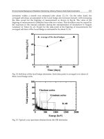
with increasing sample size in both sampling designs. In Fig. 4 is shown the relationship
between bias and sample size of Shannon’s diversity estimator in systematic and random
sampling designs.


Fig. 4. The relationship between bias and sample size of Shannon’s diversity estimator using
point sampling method in systematic and random sampling designs (from Ramezani et al.,
2010).
-6
-5
-4
-3
-2
-1
0

0 100 200 300 400
Bias (%)
Sample size
Systematic design
Random design

Environmental Monitoring
212
In line intersect sampling, similar to point sampling, both RMSE and bias of Shannon’s
estimator tended to decrease with increasing sample size and line length. The longer line
transect (here 150 m) resulted in lower RMSE and bias than shorter one (here 37.5 m), for a
given sample size. We found a small and negative bias for the estimator in both point and
the LIS methods. The magnitude of bias tended to decrease both with increasing sample size
and line transects length. Straight line configuration resulted in lower RMSE and bias than
other configurations.
3.2 Total edge length
In point sampling, the magnitude of RMSE of estimator is highly related to buffer width, for
a given sample size and a wide buffer resulted in lower RMSE than narrow one. The edge
length estimator had bias since parts of buffer close to the map border were outside the
map. Bias of estimator tended to increase with increasing buffer width whereas it was
independent on sample size. To eliminate or reduce the bias of estimator three corrected
methods were suggested which have been discussed in detilas in Ramezani et al. (2010).
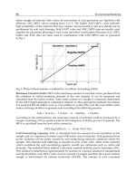
In LIS, the magnitude of RMSE of estimator is dependent on the length of the line transect,
for a given sample size and the longer transect resulted in lower RMSE than short one.
Furthermore, straight line configuration resulted in lower RMSE compared to other
configurations (e.g., L and square shape). In Fig. 5 is shown the relationship between
relative RMSE and sampling line lengths of total edge length estimator.


Fig. 5. Relative RMSE of total edge length estimator for different sampling line lengths and

configurations of line intersect sampling, for a given sample size (from Ramezani and Holm,
2011c).
3.3 Contagion
Point based contagion (i.e., Eq. 7) is a distance–dependent function that delivers a contagion
value that decreased with increasing point distance. The rate of decrease of the contagion
value was faster in a fragmented landscape compared to a more homogenous landscape.
Examples of such landscapes are shown in Fig. 6. The contagion estimator was biased even
20
30
40
50
60
70
80
90
25 75 125 175
RMSE (%)
Sampling line length per configuration (m)
straight line
L - shape
Y - shape
Triangle shape
Square shape
Landscape Environmental Monitoring:
Sample Based Versus Complete Mapping Approaches in Aerial Photographs
213
if its component (i.e., ( )
ij
p
d ) was estimated without bias. The sources of bias discussed in

details in Ramezani and Holm (2011b).




Fig. 6. Example of two landscapes with different degree of fragmentation and their
corresponding contagion function (Eq. 7). Top: a high fragmented landscape (four land
cover class and nineteen patches) with large rate of decrease of the contagion function.
Bottom: a homogenous landscape (three land cover class and three patches) with a small
rate of decrease in the contagion function.
In line intersect sampling, both RMSE and bias of the contagion estimator (Eq.8) tended to
decrease with increasing sample size and line transects length. Straight line configuration
resulted in lower RMSE and bias than other configurations. We found a small and negative
bias for the contagion estimator despite its components (i.e.,
ˆ
i
j
E
and
ˆ
t
E
) can be estimated
without bias. The relative RMSE and bias of the contagion estimator through line intersect
sampling (LIS) method (Eq.8) is shown in Fig. 7. Note that the two contagion estimators
differ as they are based on different equations (i.e., Eqs.7 and 8).
A comparison was also made for variability in terms of range and mean in sample based
estimates of Shannon’s diversity, edge length and contagion metrics for sample sizes 16 and
100. In Table 1 is provided an example for line intersects sampling method, systematic
sampling design, straight line configuration and line length 37.5 m.

0.8
0.8
0.9
0.9
0.9
0.9
0 100 200 300
Contagion
Point distance (m)
0
0.2
0.4
0.6
0.8
1
0 100 200 300
Contagion
Point distance (m)

Environmental Monitoring
214


Fig. 7. Relative RMSE (top) and bias (bottom) of contagion estimator (Eq. 8) for different
sampling line lengths and configurations, a sample 49 and systematic sampling design

Landsca
p
e metrics

Sam
p
le size
16

100
Shannon’ diversit
y
0.398
(
0.019-0.747
)
0.423
(
0.026-0.784
)

Conta
g
ion
a
0.188
(
0.006-0.478
)
0.407
(
0.226-0.758
)

Total ed
g
e len
g
th
(
m ha
-1
)
92.2
(
12.2-197.6
)
92.1
(
10.5-194.6
)

a
according to Eq.8
Table 1. Variability (mean) in sample based estimates of Shannon’s diversity, edge length and
contagion in fifty random landscapes (NILS plots) in Sweden for sample sizes 16 and 100. Data
collected using line intersects sampling method, systematic sampling design, straight line
configuration and 37.5 m length of sampling lines. Ranges are given in parentheses.
3.4 Time study (cost needed for data collection)
A time study was conducted on non-delineated aerial photos from NILS employing an
experienced photo interpreter. The results of the time study for Shannon’s diversity and
total edge length are summarized in Tables 2 and 3.
15
30

45
60
75
25 75 125 175
RMSE (%)
Sampling line length per configuration (m)
Straight line
L shape
Y shape
Triangle shape
square shape
-80
-65
-50
-35
-20
25 75 125 175
Bias (%)
Sampling line length per configuration (m)

45

35

25

15

5
Square shape

0


-10

-20

-30

-40
Landscape Environmental Monitoring:
Sample Based Versus Complete Mapping Approaches in Aerial Photographs
215

Method Time needed (h)
Complete mapping 3.5
Point sampling (number of points)
9 0.4
100 0.8
225 1.9
400 3.3
Table 2. Average time consumption of data collection on five NILS plots for point sampling
and complete mapping for deriving the Shannon’s index (from Ramezani et al. (2010))

Sampling method Time needed (min)
Edge length estimator Shannon’ s diversity estimator
Point sampling 25
a
28.3
LIS 18.3

b
60
b

a
(buffer 40 (m))
b
(line 150 (m))
Table 3. Average time needed for point and line intersect sampling (LIS) methods for
deriving Shannon’s diversity and total edge length. For sample size 100 (number of point
and lines)
The time needed to collect data was highly related to landscape complexity and the
classification system applied. We also found that in a coarse classification system the time
needed was less than in a more detailed system. This issue becomes more serious in
complete mapping approaches where all potential polygons should be delineated.
Furthermore, time was also dependent on sampling method the chosen. With a point
sampling method less time was needed for estimating Shannon’s diversity compared with
other metrics. With line intersect sampling; it was more time efficient to use edge-related
metrics. For a given sample size, the time depended on the length of line transect (in LIS)
and the buffer width (in point sampling). With the former method it is indicated that the
time is independent on line configuration in the aerial photo.
4. Discussion
This study addresses the potential of sampling data for estimating some landscape metrics
in remote sensing data (aerial photo). Sample based approach appears to be a very
promising alternative to complete mapping approach both in terms of time needed (cost)
and data quality (Kleinn and Traub, 2003; Corona et al., 2004; Esseen et al., 2006). However,
some metrics may not be estimated from sample data regardless of chosen sampling method
since currently used landscape metrics are defined based on mapped data. To describe
landscape patterns accurately, a set of landscape metrics is needed since all aspect of
landscape composition and configuration cannot be captured through a single metric. On

the other hand, all metrics cannot be extracted using a single sampling method. Thus, in a
sample based approach a combination of different sampling methods is needed, for
instance, a combination of point and line intersect sampling. In such combined design, the

Environmental Monitoring
216
start, mid and end points of line transects can be treated as grid of points which is preferred
for estimating area proportions of different land cover classes within a landscape and thus
Shannon’s diversity. It would also be effective in terms of cost if several metrics could
simultaneously be derived from a single sampling method.
From a statistical point of view unbiasedness is a desirable property of an estimator. In
sample based assessment of landscape metrics, attributes (metrics components) such as
the number, size, and edge length of patches must unbiasedly be estimated (Traub and
Kleinn, 1999) if an unbiased estimate is needed. However, this is a necessary but not
sufficient conditions (Ramezani, 2010). For instance, in the case of Shannon’ diversity,
there is still bias despite its component i.e., area proportions of land cover classes can be
estimated without bias through both point and line intersect sampling methods
(Ramezani et al., 2010; Ramezani and Holm, 2011c). The bias is due to non–linear
transformation, which also generally is the case for other metrics with non–linear
expression such as contagion. Bias of selected metric estimators is very small if the sample
size is large and the magnitude of bias depends jointly on type of selected metric, the
sampling method, and the complexity of the landscape structure. To achieve an acceptable
precision in a complex landscape there is a need for a larger sample size compared to the
homogenous landscape.
The landscape metrics used in this study are based on a patch-mosaic model where sharp
borders are assumed between patches. In such procedure, as noted by Gustafson (1998) the
patch definition is subjective and depends on criterion such as the smallest unit that will be
mapped (minimum mapping units, MMU). This becomes more challenging in a highly
fragmented landscape where smaller patches than predefined MMU are neglected. Even
though these patches constitute a small proportion (area) of the landscape, they contribute

significantly to the overall diversity of that landscape; including biodiversity where other
type organisms may occupy these patches habitats. However, in sample based approach
which can be conducted in non–delineated aerial photos, there is no need to predefine
minimum patch size and even very small patches can be included in the monitoring system.
Furthermore, point sampling appears to be in consistent with gradient based model of
landscape (McGarigal and Cushman, 2005) where landscape properties change gradually
and continuously in space and where no subjective sharp border need to be assumed
between patches.
Polygon delineation errors are common in manual mapping process. It can be assumed that
this error can be eliminated when sampling methods are used for estimating some
landscape metrics. As a result, obtained information and subsequent analysis is more
reliable than for traditional manual polygon delineation. As an example, for estimating the
metrics Shannon’s diversity and contagion using point sampling, no mapped data are
needed and assessment is only concentrated on sampling locations. This is also true for the
LIS, for instance, the total length estimation of linear features within a landscape is to be
based on simply counting the interactions between lines transect and a potential patch
border. Consequently, assessment is conducted along line transect which, thus, considerable
reduce the polygon delineation error.
It is clear, however, that a sample based approach cannot compete with a complete mapping
approach, in particular when high quality mapped data is available. With the mapping
approach a suite of metrics can be calculated for patch, class, and landscape levels whereas
in sample based approach a limited number of metrics on landscape level can often be
estimated.
Landscape Environmental Monitoring:
Sample Based Versus Complete Mapping Approaches in Aerial Photographs
217
5. Conclusion
A sample based approach can be used complementary to complete mapping approach, and
adds a number of advantages, including 1) the possibility to extract metrics at low cost 2)
applicable in case of lacking categorical map of entire landscape 3) the possibility in some

case to obtain more reliable information and 4) the possibility of estimating some metrics
from ongoing field-based inventory such as national forest inventories (NFI). In some cases,
there is a need to slightly redefine currently used landscape metrics or develop new metrics
to meet sample data. There is obviously plenty of room for further studies into this topic
since sample based assessment of landscape metrics is a new approach in landscape
ecological surveys.
6. References
Blaschke, T., (2004). Object-based contextual image classification built on image
segmentation: IEEE Transactions on Geoscience and Remote Sensing, p. 113-119.
Bunce, R.G.H., Metzger, M.J., Jongman, R.H.G., Brandt, J., de Blust, G., and Elena-Rossello,
R., et al., (2008). A standardized procedure for surveillance and monitoring
European habitats and provision of spatial data: landscape Ecology, v. 23, p. 11-25.
Cochran, G., (1977). Sampling techniques: New York, Wiley, xvi, 428 p.
Corona, P., Chirici, G., and Travaglini, D., (2004). Forest ecotone survey by line intersect
sampling: Canadian Journal of Forest Research-Revue Canadienne De Recherche
Forestiere, v. 34, p. 1776-1783.
Esseen, P.A., Jansson, K.U., and Nilsson, M., (2006). Forest edge quantification by line
intersect sampling in aerial photographs: Forest Ecology and Management, v. 230,
p. 32-42.
Fischer, J., and Lindenmayer, D.B., (2007). Landscape modification and habitat
fragmentation: a synthesis: Global Ecology and Biogeography, v. 16, p. 265-280.
Gregoire, T.G., and Valentine, H.T., (2008). Sampling Strategies for Natural Resources and the
Environment Boca Raton, Fla. London, Chapman & Hall/CRC.
Gustafson, J.E., (1998). Quantifying landscape spatial pattern: What is the state of the art?:
Ecosystems, v. 1, p. 143-156.
Hanski, I., (2005). Landscape fragmentation, biodiversity loss and the societal response - The
longterm consequences of our use of natural resources may be surprising and
unpleasant: Embo Reports, v. 6, p. 388-392.
Jansson, K.U., Nilsson, M., and Esseen, P A., (2011). Length and classification of natural and
created forest edges in boreal landscapes throughout northern Sweden: Forest

Ecology and Management.v.262,P.461-469
Kleinn, C., and Traub, B., (2003). Describing landscape pattern by sampling methods, in
Corona, P., Köhl, M., and Marchetti, M., eds., Advances in forest inventory for
sustainable forest management and biodiversity monitoring., Volume 76, p. 175-189.
Li, H., and Reynolds, J., (1993). A new contagion index to quantify spatial patterns of
landscapes: Landscape Ecology, v. 8, p. 155-162.
Matérn, B., (1964). A method of estimating the total length of roads by means of line survey:
Studia forestalia Suecica, v. 18, p. 68-70.
McGarigal, K., and Cushman, S.A., (2005). The gradient concept of landscape structure, in
Wiens, J., and Moss, M., eds., Issues and perspectives in landscape ecology: Cambrideg,
Cambrideg University press.

Environmental Monitoring
218
McGarigal, K., and Marks, E.J., (1995). FRAGSTATS: Spatial pattern analysis program for
quantifying landscape pattern. General Technical Report 351. U.S. Department of
Agriculture, Forest Service, Pacific Northwest Research Station.
Morgan, J., Gergel, S., and Coops, N., (2010). Aerial Photography: A Rapidly Evolving Tool
for Ecological Management: BioScience, v. 60, p. 47-59.
NIJOS, (2001). Norwegian 3Q Monitoring Program: Norwegian institute of land inventory.
O’Neill, R.V., Krumme, J.R., Gardner, H.R., Sugihara, G., Jackson, B., DeAngelist, D.L.,
Milne, B.T., Turner, M., Zygmunt, B., Christensen, S.W., Dale, V.H., and Graham,
L.R., (1988). Indices of landscape pattern: Landscape Ecology v. 1, p. 153-162.
Raj, D., (1968). Sampling theory: New York, McGraw-Hill, 302pp. p.
Ramezani, H., (2010). Deriving landscape metrics from sample data (PhD thesis): Umeå,
Swedish University of Agricultural Sciences (SLU).
Ramezani, H., and Holm, S., (2011a). A distance dependent contagion functions for vector-
based data: Environmental and Ecological Statistics (accepted).
—, (2011b). Estimating a distance dependent contagion function using point sample data (in
review).

—, (2011c). Sample based estimation of landscape metrics: accuracy of line intersect
sampling for estimating edge density and Shannon’s diversity . Environmental and
Ecological Statistics, v. 18, p. 109-130.
Ramezani, H., Holm, S., Allard, A., and Ståhl, G., (2010). Monitoring landscape metrics by
point sampling: accuracy in estimating Shannon’s diversity and edge density:
Environmental Monitoring and Assessment v. 164, p. 403-421.
Ries, L., Fletcher, R.J., Battin, J., and Sisk, T.D., (2004). Ecological responses to habitat edges:
Mechanisms, models, and variability explained: Annual Review of Ecology
Evolution and Systematics, v. 35, p. 491-522.
Riitters, K.H., O'Neill, R.V., Hunsaker, C.T., Wickham, J.D., Yankee, D.H., Timmins, S.P.,
Jones, K.B., and Jackson, B.L., (1995). A factor-analysis of landscape pattern and
structure metrics: Landscape Ecology, v. 10, p. 23-39.
Saura, S., and Martinez-Millan, J., (2001). Sensitivity of landscape pattern metrics to map
spatial extent: Photogrammetric Engineering and Remote Sensing, v. 67, p. 1027-
1036.
Ståhl, G., Allard, A., Esseen, P A., Glimskär, A., Ringvall, A., Svensson, J., Sture Sundquist,
S., Christensen, P., Gallegos Torell , Å., Högström, M., Lagerqvist, K., Marklund, L.,
Nilsson, B., and Inghe, O., (2011). National Inventory of Landscapes in Sweden
(NILS) - Scope, design, and experiences from establishing a multi-scale biodiversity
monitoring system: Environmental Monitoring and Assessment v. 173, p. 579-595.
Takács, G., and Molnár, Z., (2009) National biodiversity monitoring system XI. Habitat
mapping (2nd modified ed., p. 54). Ministry of Environment and Water, Budapest.
Traub, B., and Kleinn, C., (1999). Measuring fragmentation and structural diversity:
Forstwissenschaftliches Centralblatt, v. 118, p. 39-50.
Wickham, J.D., Riitters, K.H., ONeill, R.V., Jones, K.B., and Wade, T.G., (1996). Landscape
'contagion' in raster and vector environments: International Journal of
Geographical Information Systems, v. 10, p. 891-899.
Wulder, M.A., White, J.C., Hay, G.J., and Castilla, G., (2008). Towards automated
segmentation of forest inventory polygons on high spatial resolution satellite
imagery: Forestry Chronicle, v. 84, p. 221-230.

14
Real-Time Monitoring of Volatile
Organic Compounds in Hazardous Sites
Gianfranco Manes
1
, Giovanni Collodi
1
, Rosanna Fusco
2
,
Leonardo Gelpi
2
, Antonio Manes
3
and Davide Di Palma
3
1
Centre for Technology for Environment Quality & Safety, University of Florence,
2
eni SpA,
3
Netsens Srl,
Italy
1. Introduction
Volatile Organic Compounds (VOCs) are largely used in many industries as solvents or
chemical intermediates. Unfortunately, they include some components, present in the
atmosphere, that can represent a risk factor for human health. They are also present as a
contaminant or a by-product in many processes, i.e. in combustion gas stacks and
groundwater clean-up systems.
Benzene, in particular, shows a high toxicity resulting in a Time-Weighted Average

(TWA) limit of 0.5 ppm, as compared, for instance, with TWA for gasoline, in the range of
300 ppm.
Detection of VOCs at sub-ppm levels is, thus, of paramount importance for human safety
and industrial hygiene in hazardous environments.
The commonly used field-portable instruments for VOC detection are the hand-held
Photo-Ionisation Detectors (PIDs), sometime using pre-filter tubes for specific gas detection.
PIDs are accurate to sub-ppm, measurements are fast, in the range of one or two minutes
and, thus, compatible with on-field operation. However, they require skilled personnel and
cannot provide continuous monitoring.
Wireless connected hand-held PID Detectors start being available on the market, thus
overcoming some of the previously described limitations, but suffering for the limited
battery life and relatively high cost.
The paper describes the implementation and on-field results of an end-to-end distributed
monitoring system integrating VOC detectors, capable of performing real-time analysis of
gas concentration in hazardous sites at unprecedented time/space scale.
The system consists of a Wireless Sensor Network (WSN) infrastructure, whose nodes are
equipped with distributed meteo-climatic sensors and gas detectors, of TCP/IP over GPRS
Gateways forwarding data via Internet to a remote server and of a user interface which
provides data rendering in various formats and access to data.
The paper provides a survey of the VOC detector technologies of interest, of the state-of-the-
art of the fixed and area wireless technologies available for Gas detection in hazardous areas
and a detailed description of the WSN based monitoring system.

Environmental Monitoring

220
2. Regulatory requirements for oil&gas industry
The oil&gas sector is characterised by a high complexity in terms of processes, materials and
final products. Consequently, activities related to the oil&gas industry need to be effectively
controlled to minimize their impact on the environmental matrices (air, water and soil) and

to avoid any potential risks for human health.
Environmental issues related to the oil&gas sector are also strictly dependent on the specific
activities performed. In particular, petrochemical and refining sectors are involved in the
production of waste materials, such as water and toxic sludge, and atmospheric pollutant
emissions, including many VOCs potentially harmful both to the environment and to
human health. All these environmental issues are considered areas of high human and
environmental risk and therefore subject to stringent international and local environmental
regulations.
During the last decade the EU has fixed several Thematic Strategies to improve the
management and control on Air Pollution, Soil Protection, Prevention and Recycling of
Waste as a follow-up to the Sixth Community Environment Action Programme (Council of
22
nd
July 2002). In particular, the EU set objectives and regulations on the industrial sector to
protect human health and the environment, objectives can be met only with further
reductions in emissions arising from industrial activities. The final act of this process was
the publication, on 24
th
November 2010, of the new Directive 75/2010 (IED) on industrial
emissions (integrated pollution prevention and control) which recasts together six directives
on industrial emissions (IPPC, LCP, VOC, TiOxide).
Based on the principle of the polluter pays and also on the pollution prevention one, industrial
owners should manage their activities in order to protect the environment as a whole, in
compliance to the IPPC integrated approach. Furthermore, in accordance with the Århus
Convention on access to information and public participation, operators should both
improve and promote tools and procedures, such as adopting environmental management
system (ISO 14001), increasing the accountability and transparency of the monitoring and
reporting data process and contributing to public awareness of environmental issues, and
support for the decisions taken.
In order to ensure the prevention and control of pollution, each installation should operate

only if it holds a permit, which should include all the measures necessary to achieve a high
level of protection of the environment as a whole, and to ensure that the installation is
operated in accordance with the general principles governing the basic obligations of the
operator. The permit should also include emission limit values for polluting substances or
technical measures and monitoring requirements; all conditions should be set on the basis of
Best Available Techniques (BAT)
1
applied on each specific installation.
On the other hand, the European Union has issued, in 2008, Directive No 2008/50/EC
concerning ambient air quality and cleaner air for Europe.
In order to protect human health and mostly urban environment, the directive addresses the
following key points:

1
In the IPPC Directive, BAT are defined as “the most effective technologies available for achieving a
high level of environmental protection concerned in an economically feasible and technical view of the
costs and benefits”. Currently BAT is identified on the basis of an exchange of information organized by
the European Commission that occurs between the Member States, industry and non-governmental
organisations

Real-Time Monitoring of Volatile Organic Compounds in Hazardous Sites

221
 It’s very important to prevent and reduce pollutant emissions at source, implementing
the best effective reduction measures, both technological and on management.
Emissions of air pollutant should be reduced by each member state according to World
Health Organisation guidelines.
 The directive establishes the need of a strong monitoring system and the reciprocal
exchange of information and data from networks and individual stations measuring
ambient air pollution in order to incorporate the latest health and scientific

developments and the experience of the Community.
 Each Member State should ensure consistency and representativeness of the
information collected on air pollution; standardised measurement techniques and
common criteria for the number and location of measuring stations are defined.
 For assessing air quality, information and data collected from fixed measurement
stations may be integrated with data from alternative techniques, such as modelling or
indicative measurements. The use of measurement methods other than standardised
methods allows improving data monitoring and interpretation in some critical areas
(such as, for instance, industrial sites) in an economical and feasible way.
Alternative measurement methods may provide indicative results that could be less
accurate than those made with the reference method. Indicative measurement techniques
based on the use of automatic sensors, mobile laboratories, portable analysers and manual
methods of measurement, such as diffusive sampling techniques, are very interesting due to
the relatively low cost and simplicity of operation compared with instrumental and
operative costs of fixed measuring stations.
3. Volatile Organic Compounds
Volatile Organic Compounds are defined as all compounds containing organic carbon
characterized by low vapour pressure at ambient temperature. They are present in the
atmosphere mainly in the gas phase.
The number of volatile organic compounds observed in the atmosphere, both in urban and
remote areas, is extremely high and includes, in addition to hydrocarbons (compounds
containing only carbon and hydrogen), also oxygen species such as ketones, aldehydes,
alcohols, acids and esters. Natural emissions of VOCs include the direct emissions from
vegetation and the degradation of organic matter; anthropogenic emissions are mainly
caused by the incomplete combustion of hydrocarbons, the evaporation of solvents and
fuels, and processing industries. On a global scale, natural and anthropogenic emissions of
VOCs are of the same order of magnitude.
A lot of volatile organic compounds are highly toxic; this makes them extremely dangerous
to human health. In addition, many compounds react with nitrogen oxides and other
substances, contributing to the formation of ozone in the lower atmosphere, with impact on

climate change and pollution issues (i.e. photochemical smog). Finally, some substances are
characterized by a very low odour threshold, resulting in complaints from population and
community living around industrial sites.
4. VOC classification
There are many classification systems, based on chemical characteristics, or based on the
impact on the environment and human health. The term VOC covers several groups of

Environmental Monitoring

222
organic substances with different chemical and physical characteristics. VOC compounds
include in fact compounds containing only atoms of carbon and hydrogen (which include
for example aromatic compounds such as benzene). One type of classification used in many
states is defined by German regulations (TA Luft - Technical Instructions on Air Quality
Control): it identifies three classes of VOCs based on their impact and it defines appropriate
prevention and control.
The three classes are:
 extremely hazardous to health – such as benzene, vinyl-chloride and 1,2 dichloroethane
 class A Compounds – that may cause significant harm to the environment (e.g.
acetaldehyde, aniline, benzyl chloride)
 class B Compounds – that have lower environmental impact.
Benzene (C6H6) is a volatile organic compound belonging to the family of hydrocarbons
and characterized by a monocyclic aromatic structure. It is a natural constituent of
petroleum, and it is present in gasoline by virtue of its anti-knock properties (it contributes
to increase octane number).




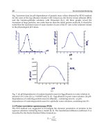
Fig. 1. VOC emission distribution in Italy

In the chemical industry, benzene is a solvent widely used, especially as an intermediate for
the synthesis of other products (ethylbenzene, cumene, cyclohexane, etc.) in turn used for
the production of plastics, resins, paints, tires, detergents etc.
Benzene exposure is very dangerous to human health; it is classified as a human carcinogen,
due to the high toxicity. Among VOCs, benzene is the only compound for which the
European directive on air quality has set a limit to 5 g/m
3
(about 1.5 ppb), with no margin
of tolerance. At work, the TLV-TWA limit is set at 0.5 ppm for prolonged exposure of 8
hours per day and 2.5 ppm for exposures not exceeding 15 minutes (for reference TLW-
TWA for gasoline is in the range of 300 ppm).
Benzene emissions related to petroleum activities are about 5% of total emissions, while for
the non-methane VOCs the chemical industry appears to be more involved than refining
sector.
The graphs in Fig. 1 (2008 VOC and Benzene emission distribution in Italy - data from
ISPRA Database) show that motor vehicles are the main pollution sources for benzene,
while painting is the main source for non-methane VOCs.

Real-Time Monitoring of Volatile Organic Compounds in Hazardous Sites

223
Main VOC sources in petroleum industry
Oil installations, petrochemical plants and refineries are industrial sites that manage several
raw materials (crude oil, natural gas, chemical intermediates, etc.), thus having great impact
on the environment. Industrial processes may generate VOC emissions to the atmosphere,
so prevention and control is becoming a very important issue in the petroleum industry.
The main quantity of VOC releases are due to diffuse and fugitive emission sources. The
main sources of VOCs from refineries and petrochemicals are fugitive emission from piping,
vents, flares, air blowing, waste water system, storage tanks and handling activities, loading
and unloading systems.

Fugitive emissions from piping
Fugitive emissions are defined as emissions of pollutants (gases and dust) in the atmosphere
resulting from losses such as pumps, valves, flanges, drains, compressors, sampling points,
open ended lines, agitators. The loss of process fluids affects all plant equipment; although
the amount emitted from single components may be individually small, the cumulative
emissions of the plant can be considerable in some cases.
Fugitive emissions can be considered as the main source of VOCs in the refinery. The
application of Best Available Techniques requires industrial facilities to define a Leak
Detection and Repair programme (LDAR), which allows the monitoring at defined
frequency of the leaks from plant’s component, thus providing a swift repair of leaker.
A standard method (EPA 21) is available to define the monitoring criteria. In addition, it is
possible to calculate fugitive emissions based on average literature data, but this approach
does not provide evidence of improvements and does not allow for leaker repair. For this
reason, on-site monitoring is mandatory.
Handling and storage tanks
VOC emissions from storage tanks are due to evaporative loss of the hydrocarbon liquid
stored. There are two main types of tanks, fixed roof and floating (internal or external) roof
tanks. In the first case, evaporation losses occur mainly from vents and fittings. In floating
roof tanks, where the roof is in direct contact with the liquid, emissions may occur from the
seals, especially during changes of liquid level.
Emissions depend on the type of product stored and the vapour pressure of the product:
higher vapour pressure tends to generate higher VOC emissions.
The emissions are generally estimated by calculation software that takes into account
numerous factors such as construction types (type of the roof, seals, colour, etc.), number of
loading and unloading cycles, etc.
It is possible to perform monitoring with analytical instrumentation, as long as the
requirements of intrinsically safe regulations (ATEX) are met.
During loading, i.e. product stored on vessels, VOC emissions may occur in the vapour
phase.
Waste Water Treatment Plants

VOC emissions from Waste Water Treatment Plants are due to evaporation of more volatile
compounds from tanks, ponds and sewerage system drains.
Because of contamination of treated water, this type of plant is a major source of odorous
emissions, thus causing the need for careful monitoring and control. VOCs are emitted also
during air stripping in flotation units and in the biotreaters. Emissions of VOCs and other
pollutants into the atmosphere from the treatment ponds and basins can be significantly

Environmental Monitoring

224
limited by implementing systems of coverage (almost all industrial sites have this
requirement from local authority).
Flare systems
VOC emissions are due to an incomplete combustion of flare gas. However, this type of
source does not represent a major cause of VOC emissions.
From a first analysis of the major sources, it is clear that VOC emissions come from
widespread areas inside the industrial site. The individual emission sources may have small
or large impact, but it is important to consider the overall impact of all sources combined.
Often a regular monitoring at the source may be ineffective, and sometimes the use of
methods of monitoring network in the areas close the critical area could be of great help to
combat the phenomenon and to achieve a significant reduction of emissions in an
economically feasible way.
VOC monitoring systems
Common VOC concentration measurement methods include colorimetric tubes, Infrared
Detectors, Photo Ionisation Detectors (PIDs) and Flame Ionisation Detectors (FIDs),
portable/transportable Gas Chromatograph (GC) and sampling followed by laboratory
analysis. Deployable sensors are of particular relevance, as they are capable to provide on-
site monitoring.
Sampling and laboratory analysis
The main sampling technologies for subsequent laboratory analysis are based on the use of

active and passive samplers. In the first case, sampling is done by exposing a trap in the site
under investigation connected with a pump capable of sucking a steady flow of air. The trap
is usually made of absorbent material, e.g. charcoal. The exposure time may vary from a
few tens of minutes to hours. The sample is then analysed in the laboratory with gas
chromatography techniques (GC).
Passive samplers instead use the diffusive properties of substances dispersed in the
atmosphere. They are generally exposed to ambient air for even longer periods (days,
weeks), and they are protected in order to prevent damage and contamination caused by
weather phenomena (wind, rain). The pollutants are captured at different rates because each
of them has different diffusive properties. Sample is then desorbed and analysed in the
laboratory (GC). The sampler can be treated with appropriate reagents, in order to obtain
selectivity only on a few compound families.
Various passive sampling devices are commercially available. One of the most popular is
the sampler Radiello, characterized by radially distributed operation and a better sensitivity
due to increased diffusive surface.
The difference between the two types of samplers is linked to the range of compounds they
are able to detect; passive sampler are not useful to detect many VOCs (olefins, compounds
with less than 5 atoms of carbon, etc.) because they tend not to remain adherent to the
passive diffusion sampler, due to prolonged exposure to the atmosphere. The use of one or
another depends on the family of VOCs under study.
The main advantage of this sampling technology is the low cost of materials and resources,
giving the opportunity to create very dense monitoring networks in an economical feasible
way. The disadvantage is the impossibility to continuously collect real-time data, so they are
not suitable for emergency management and early warning, but they may be useful for air
characterization of an hazardous industrial site, in terms of average concentrations and

Real-Time Monitoring of Volatile Organic Compounds in Hazardous Sites

225
emission source profiles. Another important application is the use in monitoring networks

for checking compliance with the TWA for toxic component (e.g. Benzene).
On-field monitoring
On-field monitoring technologies allow obtaining real-time concentration of pollutants close
to a specific source or along the perimeter of the industrial establishment, enabling to
manage specific emergency situations in real-time.
The equipment usually yields a response in terms of quantitative concentration levels of
VOCs in the atmosphere; in some cases it is even possible to get a specification of the
components in the air.
Below an overview of the main methods used on-site, especially at industrial sites, is carried
out.
VOC fixed analysers
The use of automatic VOC GC analysers able to collect air samples at regular intervals and
analyse them is particularly common when performing monitoring campaigns using fixed
stations or a mobile laboratory.
Mobile laboratories (as well as transferable measuring stations) usually combine the
advantages of automated measurement methods with the mobility and flexibility.
Many commercially available VOC analysers can be used to perform the task. Unlike active
and passive samplers, in this case air sampled is pumped through a sampling probe and is
sent directly to the instrument, to run GC analysis by using several detection technologies
(photo ionization, flame ionization, thermal conductivity, etc.). The measurement interval is
in the range of tens of minutes.
This methodology allows quick answers as well as concentrations for individual compounds
to be achieved; however, it does not allow simultaneous monitoring over an industrial site
grid, due to the high costs of devices (ten thousand Euros) and operation/ maintenance cost
and complexity; furthermore, to cover all the families of compounds of interest - BTEX, C1-
C6, sulphur, etc. – more than one analyser is needed.
VOC portable analysers
Portable VOC analysers are instruments of limited size and weight, easily transportable by
an operator in the plant and able to provide real-time analysis of gas concentration in
hazardous sites.

They are usually equipped with battery life in the range 8-12 hours and allow the storage of
data acquired in a time-programmable internal logger. The main application in industry is
the detection of gas leaks, leaks from piping, releases in proximity of storage tanks,
monitoring of loading and unloading areas, etc.
Based on the sensor technology, they can be classified in the main following typologies.
a. PID - Photo Ionization Detectors. These detectors are equipped with a lamp emitting
ultraviolet light. The emitted light ionizes targeted VOCs in the air sample so they can be
detected and reported as a concentration. Depending on the features of the lamp (there
are many on the market able to ionize VOCs depending on ionisation potential), a
portable PID can detect a wide range of VOC substances. The analyser is not selective but
generally provides a cumulative figure of VOCs; however, knowing emission profiles or
mixture composition (in the case of measures directly at the source, such as for fugitive
emissions from the plant components), concentration values can be calculated for each
substance by applying the response factors. It is usually possible to attach a pre-filter tube
to allow detection and selective measurement of a single VOC component (eg. Benzene).