Expert Systems for Human Materials and Automation Part 12 pptx

Expert System Based Network Testing

321
where the cut-off y
α
is found by equalizing the Kolmogorov cdf K
η
(y) and 1-α:

1
n
Pr( nD
y
)K(
y
)1
y
K(1 )
−
αηα α η
≤= =−α⇒ =−α (5)
Otherwise the null-hypothesis should be accepted at the significance level of α.
Actually, the significance is mostly tested by calculating the (
two-tail [12]) p-value (which
represents the probability of obtaining the test statistic values equal to or greater than the
actual ones), by using the theoretical
K
η
(y) cdf of the test statistic to find the area under the
curve (for continuous variables) in the direction of the alternative (with respect to

H
0
)
hypothesis, i.e. by means of a look-up table or integral calculus, while in the case of discrete
variables, simply by summing the probabilities of events occurring in accordance with the
alternative hypothesis at and beyond the observed test statistic value. So, if it comes out that:

n
p1K(nD)
η
=− <α (6)
then the null hypothesis is again to be rejected, at the presumed significance level α,
otherwise (if the p-value is greater than the threshold α), the null hypothesis is not to be
rejected and the tested difference is not statistically significant.
3.3.2 Identifying stationary intervals
While the main applications of the one-sample K-S test are testing goodness of fit with
normal and uniform distributions, the two-sample K-S test is widely used for nonparametric
comparing of two samples, since it is sensitive to differences in both location and shape of
the empirical cdfs of two samples, so it is the most important theoretical tool for detecting
change-points.
Let us now consider the test for the series
12 m
, , ,
ξξ ξ
of the first sample, and
12 n
, , ,
η
ηη of
the second, where the two series are independent. Furthermore, let

m
ˆ
F(x)
ξ
and
n
ˆ
G(
y
)
η
be the
corresponding empirical cdfs. Then the K-S statistics is:

m,n m n
x
ˆ
ˆ
DF(x)G(
y
)
sup
ξη
=− (7)
The limit distribution theorem states that:

m,n
m,n
mn
PDzK(z),0z

mn
lim
ζ
⎛⎞
<= <<∞
⎜⎟
⎜⎟
+
⎝⎠
→∞
(8)
where again
K
ζ
(z) is the Kolmogorov cdf.
3.3.3 Estimation of the (normal) distribution parameters
Let us consider a normally distributed random variable
2
N(m, )
ξ
∈σ, where:

()
()
2
2
xm
2
1
px e

2
−
−
σ
ξ
=
πσ
(9)
Its cdf
()
x
ξ
Φ can be expressed as the standard normal cdf
()
xΦ [12] of the ξ-related zero-
mean normal random variable, normalized to its standard deviation
σ:

Expert Systems for Human, Materials and Automation

322

()
()
2
2
2
xm
um
v

x
2
2
1xm1
xPr(x) e du edv
22
ξ
−
−
σ
−
−
σ
−∞ −∞
−
⎛⎞
Φ=ξ≤= =Φ =
⎜⎟
σ
πσ πσ
⎝⎠
∫∫
(10)
Normal cdf has no lower limit, however, since the congestion window can never be negative,
here we must consider a truncated normal cdf. In practice, when the congestion window
process gets in its stationary state, the lower limit is hardly 0. Therefore, for the reasons of
generality, here we consider a truncated normal cdf with lower limit
l, where l 0≥ .
Now we estimate the parameters m, σ and l, starting from:

2
lm
v
2
lm 1 lm
Pr( l) 1 1 e dv Q
2
−
σ
−
−∞
−−
⎛⎞ ⎛⎞
ξ> = −Φ = − =
⎜⎟ ⎜⎟
σσ
π
⎝⎠ ⎝⎠
∫
(11)
where:
lm
Q
−
⎛⎞
⎜⎟
σ
⎝⎠
is the Gaussian
tail function [12].

The conditional expected value of
ξ, just on the segment (l,
+∝
) is:

()
2
2
um
2
l
1
E( / l) u e du
lm
2Q
−
+∝
−
σ
ξξ> = ⋅
−
⎛⎞
πσ⋅
⎜⎟
σ
⎝⎠
∫
(12)
By substituting:
um

v, du dv
−
==σ⋅
σ
into (12.), we obtain:

()
2
22
2
2
v
2
lm
vv
22
lm lm
v
2
lm
1lm
2
11
E( / l) v m e dv
lm
2
Q
1m1
vedv edv
lm lm

22
QQ
1
vedvm
lm
2
Q
1
em
lm
2
Q
+∝
−
−
σ
+∝ +∝
−−
−−
σσ
+∝
−
−
σ
−
⎛⎞
−
⎜⎟
σ
⎝⎠

ξξ> = σ⋅+ =
−
⎛⎞
π
⎜⎟
σ
⎝⎠
σ
=+=
−−
⎛⎞ ⎛⎞
ππ
⎜⎟ ⎜⎟
σσ
⎝⎠ ⎝⎠
σ
=+=
−
⎛⎞
π
⎜⎟
σ
⎝⎠
σ
=+
−
⎛⎞
π
⎜⎟
σ

⎝⎠
∫
∫∫
∫
(13)
Now, if we pre-assign a certain value
γ to the above used tail function Q(·), then the
corresponding argument (and so
m) is determined by the inverse function Q
-1
(γ):

()
1
lm
QmlQ
−
−
⎛⎞
=
γ
⇒ =−σ⋅
γ
⎜⎟
σ
⎝⎠
(14)

Expert System Based Network Testing

323
so that (13.) can now be rewritten as:

()
2
1
1
Q
2
1
mE(/ l) e
2
−
⎡
⎤
−γ
⎣
⎦
σ
=ξξ>−⋅
γ
π
(15)
Substituting
m from (14.) into (15.) results with the following formula for σ:

()
()
2
1

1
Q
1
2
lE(/ l)
1
Qe
2
−
⎡
⎤
−γ
⎣
⎦
−
−
ξξ
>
σ=
γ−
πγ
(16)
Finally, substituting the above expression for
σ into (14.), we obtain the expression for m:

()
()
()
()
2

1
2
1
1
Q
1
2
1
Q
1
2
1
QE(/l)le
2
m
1
Qe
2
−
−
⎡
⎤
−γ
⎣
⎦
−
⎡⎤
−γ
⎣⎦
−

γ⋅ γ ξ ξ> −
π
=
γ⋅ γ −
π
(17)
So it came out that, after developing formulas (16.) and (17.), we expressed the mean
m and the
variance
σ
2
of the Gaussian random variable ξ, by the mean E( / l)
ξξ
> of the truncated cdf,
the truncation cut-off and the tabled inverse
()
1
Q
−
γ
of the Gaussian tail function, for the
assumed value
γ. As these relations hold among the corresponding estimates, too, in order to
estimate
ˆ
m and
ˆ
σ , we need to first estimate
ˆ
E( / l)

ξξ
> and
ˆ
γ
from the sample data:

()
()
q
ii i
i1
r
ii
i1
Nl
ˆ
E( / l)
Nl
=
=
ξξ
>
ξξ> =
ξ>
∑
∑
(18)

s
ii

i1
1
ˆ
M( l)
n
=
γ
=
ξ
≤
∑
(19)
where
N
i
and M
i
denote the number of occurrences (frequency) of particular samples being
larger and smaller-or-equal than
l, respectively, and r,s ≤ n.
So once we have estimated
ˆ
E( / l)
ξξ
> and
ˆ
γ
by (18.) and (19.), we can then calculate the
estimates
ˆ

σ and
ˆ
m by means of (16.) and (17.), which completes the estimate of the pdf (9.).
3.3.4 Results of the analysis
Initially, the network traffic was characterized with respect to packet delay variation and
packet loss – that were, expectedly, considered as significant influencers on the congestion
window. Accordingly, in many tests, for mutually very different network conditions and
between various end-points, significant packet delay variation was noticed, Fig. 14.
However, the expected impact of the packet delay variation [7], [13] on packet loss (and so
on congestion, i.e. to its window size), has not been noticed as significant, Fig. 15a, 15b.
Still, some sporadic bursts of packet losses were noticed, which can be explained as a
consequence of grouping of the packets coming from various connections. Once the buffer
of the router, using drop-tail queuing algorithm, gets in overflow state due to heavy

Expert Systems for Human, Materials and Automation

324
incoming traffic, the most of or the whole burst might be dropped. This introduces
correlation between consecutive packet losses, so that they, too (as packets themselves),
occur in bursts. Consequently, the packet loss rate alone does not sufficiently characterize
the error performance. (Essentially, “packet-burst-error-rate” would be needed, too,
especially for applications sensitive to long bursts of losses [7], [9] [10], [13]).


Fig. 14. Typical packet delay variation within a test LAN segment


Fig. 15a. Typical time-diagram of correlated packet jitter and loss measurements

Fig. 15b. Typical histogram of correlated packet jitter and loss measurements
With this respect, one of our observations (coming out from the expert analysis tools we
referenced in Section 2) was that, in some instances, congestion window values show strong
correlation among various connections. Very likely, this was a consequence of the above
mentioned bursty nature of packet losses, as each packet, dropped from a particular
connection, likely causes the congestion window of that very connection to be
simultaneously reduced [7], [8], [10].
In the conducted real-life analyses of the congestion process stationarity, the congestion
window values that were calculated from the TCP PDU stream, captured by protocol
analyzers, were considered as a sequence of quasi-stationary series with constant cdf that

Expert System Based Network Testing

325
changes only at frontiers between the successive intervals [12]. In order to identify these
intervals by successive two-sample K-S tests (as explained above), the empirical cdfs within
two neighbouring time windows of rising lengths were compared, sliding them along the
data samples, to finally combine the two data samples into a single test series, once the
distributions matched.
Typical results (where “typical” refers to traffic levels, network utilization and throughput
for a particular network configuration) of our statistical analysis for 10000 samples of actual
stationary congestion window sizes, sorted in classes with the resolution of 20, are
presented in Table 1 and as histogram, on Fig. 16, visually indicating compliance with the
(truncated) normal cdf, having the sample mean within the class of 110 to 130. Accordingly,
as the TCP-stable intervals were identified, numerous one-sample K-S tests were conducted
and obtained the p-values in the range from 0.414 to 0.489, which provided solid indication
for accepting (with
α=1%) the null-hypothesis that, during stationary intervals, the statistical
distribution of congestion window was (truncated) normal.

Pr(x
i
-20 <x < x
i
) 278 310 624 928 2094 2452 1684 911 478 157 63 21
x
i

30 50 70 90 110 130 150 170 190 210 230 250
Table 1. Typical values of stationary congestion window size

0
400
800
1200
1600
2000
2400
30 70 110 150 190 230
Window size
F
requency o
f
occurence

Fig. 16. Typical histogram of the congestion window
As per our model, the next step was to estimate typical values of the congestion window
distribution parameters. So, firstly, by means of (19.),
ˆ
γ

was estimated as one minus the
sum of frequencies of all samples belonging to the lowest value class (so e.g., in the typical
case, presented by Table 1 and Fig. 16
,
ˆ
γ
=1-278/10000=0.9722 was taken, which determined
the value
()
1
Q
−
γ
=-1.915 that was accordingly selected from the look-up table). Then the
value of
l=30 was chosen for the truncation cut-off and, from (18.), the mean
ˆ
E( / l)
ξξ
> =117.83 of the truncated distribution was calculated, excluding the samples from
the lowest class and their belonging frequencies, from this calculation.
Finally, based on (16.) and (17.), the estimates for the distribution mean and variance of the
exemplar typical data presented above, were obtained as:
ˆ
m =114.92 and
ˆ
σ =44.35.
4. Conclusion
It has become widely accepted that network managers’ understanding how tool selection
changes with the progress through the management process, is critical to being efficient and

Expert Systems for Human, Materials and Automation

326
effective. Among various state-of-the-art network management tools and solutions that have
been briefly presented in this chapter, as ranging from simple media testers, through
distributed systems, to protocol analyzers, specifically, expert analysis based
troubleshooting was focused as a means to effectively isolate and analyze network and
system problems. With this respect, an illustrating example of real-life testing of the TCP
congestion window process is presented, where the tests were conducted on a major
network with live traffic, by means of hardware and expert-system-based distributed
protocol analysis and applying the appropriate additional model that was developed for
statistical analysis of captured data.
Specifically, it was shown that the distribution of TCP congestion window size, during
stationary intervals of the protocol behaviour that was identified prior to estimation of the
cdf, can be considered as close to the normal one, whose parameters were estimated
experimentally, following the theoretical model.
In some instances, it was found out that the congestion window values show strong
correlation among various connections, as a consequence of intermittent bursty nature of
packet losses.
The proposed test model can be extended to include the analysis of TCP performance in
various communications networks, thus confirming that network troubleshooting which
integrates capabilities of expert analysis and classical statistical protocol analysis tools, is the
best choice whenever achievable and affordable.
5. References
[1] Comer, D. E., “Internetworking with TCP/IP, Volume 1; Principles, Protocols, and
Architecture (Fifth Edition), Prentice Hall, NJ, 2005
[2] Burns, K., „TCP/IP Analysis and Troubleshooting Toolkit“, Wiley Publishing Inc.,
Indianapolis, Indiana, 2003
[3] Oppenheimer, P. „Top-Down Network Design - Second Edition“, Cisco Press, 2004

[4] Agilent Technologies, “Network Analyzer Technical Overview”, 5988-4231EN, 2004
[5] Lipovac, V., Batos, V., Nemsic, B., “Testing TCP Traffic Congestion by Distributed
Protocol Analysis and Statistical Modelling, Promet - Traffic and Transportation,
vol. 21, issue 4, pp. 259-268, 2009
[6]Agilent Technologies, “Network Troubleshooting Center Technical Overview”, 5988-
8548EN, 2005
[7] A. Kumar,”Comparative Performance Analysis of Versions of TCP”,
IEEE/ACM
Transactions on Networking, Aug. 1998
[8] M. Mathis, J. Semke, J. Mahdavi and T. J. Ott, “The Macroscopic Behavior of the TCP
Congestion Avoidance Algorithm.” Computer Communication Review, vol. 27, no.
3, July 1997
[9] K. Chen, Y. Xue, and K. Nahrstedt, “On setting TCP’s Congestion Window Limit in
Mobile ad hoc Networks”, Proc. IEEE International Conf. on Communications,
Anchorage, May 2003
[10] S. Floyd and K. Fall,” Promoting the Use of End-to-End Congestion Control in the
Internet”, IEEE/ACM Trans. on Networking, vol. 7, issue 4, pp. 458 – 472, Aug. 1999
[11] H. Balakrishnan, H. Rahul, and S. Seshan, "An Integrated Congestion Management
Architecture for Internet Hosts", Proc. ACM SIGCOMM, Sep. 1999
[12] M. Kendall, A. Stewart, “The Advanced Theory of Statistics”
, Charles Griffin London, 1966.
[13] T. Elteto, S. Molnar, “On the distribution of round-trip delays in TCP /IP networks”,
International Conference on Local Computer Network
, 1999
0
An Expert System Based Approach for Diagnosis
of Occurr ences in Power Generating Units
Jacqueline G. Rolim and Miguel Moreto
Power Systems Group
Department of Electrical Engineering

Federal University of Santa Catarina, Florianópolis
Brazil
1. Introduction
Nowadays power generation utilities use complex information management system, as new
monitoring and protection equipment are being installed or upgraded in power plants.
Usually these devices can be configured and accessed remotely, thus, companies that
own several stations can monitor their operation from a central office. This monitoring
information is crucial in order to evaluate the power plant operation under normal and
abnormal situations. Specially in abnormal cases, like fault disturbances and generator forced
shutdown, the monitoring system data are used to evaluate the cause and origin of such
disturbance.
As the data can be accessed remotely, in general the analysis is performed at a specific
department of the utility. The engineers at this department spend, on a daily basis,
a substantial amount of time collecting and analyzing the data recorded during the
occurrences, some of them severe and others resulting from normal operation procedures.
Example of a severe occurrence is the forced shutdown of a loaded generator due to a
fault (short-circuit). Concerning normal occurrences, examples are the energization and
de-enegization procedures and maintenance tests.
The main data used to analyze occurrences are disturbance records generated by Digital Fault
Recorders (DFRs) and the sequence of events (SOE) generated by the supervisory control
and data acquisition (SCADA) system. Usually this information is accessible through distinct
systems, which complicates the analyst’s work due to data spreading. The analyst’s task is to
verify the information generated at the power stations and to evaluate whether an important
occurrence has occurred. In this case, it is also needed to identify the cause of the disturbance
and to evaluate whether the generators protection systems operated as expected. Although
this investigation is usually performed off line, it has become common in case of severe
contingencies to contact the DFR specialist to ask for his advice before returning the generator
to operation. Thus the importance to perform the analysis as quickly as possible (Moreto et al.,
2009).
The excess of data that needs to be analyzed every day is a problem faced in most analysis

centers. It is of fundamental importance to reduce the time spent in disturbance analysis
as more and more data become available to the analyst as the power system grows and
technology improves (Allen et al., 2005). In practice, engineers can’t verify all the occurrences
17
2 Will-be-set-by-IN-TECH
because of the number of records generated. It should be pointed out that a significant
percentage of these disturbance records are generated during normal situations. This way,
the development of a tool to help the analysts in their task is important and subject of several
studies. Using such a tool, the severe occurrences can be analyzed in first place and an
automated analysis result leading to a probable cause of the disturbance would greatly reduce
the time spent by the analyst and improve the quality of the analysis. The remaining records
corresponding to normal situations can be archived without human intervention.
To obtain a disturbance analysis result, specialized knowledge is necessary. Interpretation of
the operative procedures of distinct power units, familiarity with the protection systems and
their expected actions are just a few skills that the analyst should dominate. Thus, this task is
suited for application of expert systems. The focus of this chapter is on the application of a set
of expert systems to automated the DFR data analysis task using also the SOE.
The DFRs are devices that record sampled waveforms of voltage and current signals,
besides the status of relays and other digital quantities related to the generator circuit. The
DFR triggers and the data is recorded when a measured or calculated value exceeds a
previously set trigger level or when the status of one or more digital inputs changes. Thus,
when a disturbance is detected a register containing pre-disturbance and post-disturbance
information is created in the DFR’s memory, (McArthur et al., 2004).
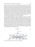
Fig. 1 shows the typical quantities monitored by a DFR. The currents on the high voltage side
of the step-up transformer (I
tf
A,B,C
), the generator terminal voltage (V
A,B,C
), the loading current

(I
A,B,C
), the neutral current/voltage (I
N
, V
N
) in addition to the field voltage and current (V
f
,
I
f
) lead to a total of 13 analog quantities per generation unit that should be verified at each
occurrence.
Fig. 1. Typical quantities monitored by DFRs in a power generation unit.
Several papers have been published in technical journals and conferences proposing and
testing schemes to automate the disturbance analysis task. However, the majority are
designed for fault diagnosis in transmission systems and for power quality studies, not
considering the characteristics of generation systems.
Davidson et al. (Davidson et al., 2006) describe the application of a multi-agent system to the
automatic fault diagnosis of a real transmission system. Some agents, based on expert systems
and model based reasoning, collect and use information from the SCADA system and from
DFRs.
328
Expert Systems for Human, Materials and Automation
An Expert System Based Approach for Diagnosis of Occurrences in Power Generating Units 3
Another paper (Luo & Kezunovic, 2005) proposed an expert system (ES) that makes use of
data from DFRs and sequence of events of digital protection relays to analyze the disturbance
and evaluate the protection performance. Expert systems are also employed in PQ studies as
in Styvaktakis (Styvaktakis et al., 2002). In this paper the disturbance signal is segmented into
stationary parts that are used to obtain the input data for the ES.

When applied to automated disturbance analysis of power systems, computational
intelligence techniques are normally used in conjunction with techniques for feature
extraction. The most common ones are the Fourier Transform (Chantler et al., 2000), Kalman
Filters (Barros & Perez, 2006) and the Wavelet Transform (Gaing, 2004).
In this chapter we propose a scheme to automatically detect and classify disturbances in
power stations. Two sources of information are used: disturbance records and sequence of
events. The first objective of this scheme is to discriminate the DFR data that do not need
further analysis from the ones resulting from serious disturbances. To do this the phasor
type of disturbance record is used. The SOE is used in the scheme to complement the result
obtained by the DFR data. Examples of incidents that do not require further analysis are:
DFR data resulting from a voltage trigger during normal energization or de-energization of
a generator; a protection trigger during maintenance tests of relays while the generator is
off-line; or a trigger coming from another DFR without any evidence of fault on the monitored
signals. The second objective is to classify the disturbance, using the waveform record,
providing a diagnosis to help the analysts with their task.
The proposed methodology has been developed with collaboration from a power generation
utility and a DFR manufacturer. The module which analyses the phasor record was validated
using hundreds of DFR records generated during real occurrences in a power plant over a
period of four months while the waveform record module was tested with simulated records
and a real fault record.
Section 2 of this chapter presents a brief description of the sources of data used: Digital Fault
Recorders and the SCADA system (responsible for generating the SOE). In Section 3 an overall
view of the proposed scheme is shown. Sections 4 and 5 describe the two main modules
proposed to diagnosing the disturbances that use phasor and waveform records. Some results
and comments about the performance of the system are discussed in Section 6. Finally, some
general conclusions are stated in Section 7.
2. Data sources
Currently most power utilities have communication networks that allow remote monitoring
and control of the system. These networks make possible to access disturbance records and
supervisory data in a centralized form. Next subsections will describe these data (disturbance

records and sequence of events), which are used by the proposed scheme to automatically
classify disturbances.
2.1 Digital fault recorders
Digital fault recorders are responsible for generating oscillographic data files. An
oscillography can be viewed as a series of snapshots taken from a set of measurements (like
generator terminal voltages and currents) over a certain period of time. Usually these records
are stored in COMTRADE format (IEEE standard C37.111-1999)(IEE, 1999), when the DFR is
triggered by one of the following situations:
• The magnitude of a monitored signal reaches a previously defined threshold level.
329
An Expert System Based Approach for Diagnosis of Occurrences in Power Generating Units
4 Will-be-set-by-IN-TECH
• The rate of change of a monitored signal exceeds its limit.
• The magnitude of a calculated quantity (active, reactive and apparent power, harmonic
components, frequency, RMS values of voltage and currents, etc.) reaches the threshold
level.
• The rate of change of a calculated quantity for instance, active power, exceeds its preset
limit.
• The state of the DFR digital inputs change.
When the DFR triggers by some of the above situations, all digital and analog signals
are stored in its memory, including the pre-fault, fault and post-fault intervals. Because
the thresholds (also called triggers) are set at aiming to detect every fault, DFRs may
also be triggered during normal situations. Examples of these situations are energization
and de-energization of the machine and tests in protective relays while the generator is
disconnected.
One of the main advantages of modern DFRs is their ability to synchronize their time
stamp with the global position system (GPS) time base. Thus, in addition to synchronized
waveforms, these devices are able to calculate and store a sequence of phasors of the electrical
quantities before, during and after the disturbance. In general, one phasor is stored for each
fundamental frequency cycle. Because of this lower sampling rate, a phasor record, also called

“long duration record” may store several minutes of data, while the waveform record, called
“short duration record” only records for a few seconds.
The approach described in this chapter uses the long duration record to pre-classify the
disturbance and the waveform record to analyze the occurrences tagged as “important”. The
main reason for this choice of using firstly the phasor record is that in large generators the
transient period of disturbance signals can be considerably long (dozens of seconds or even
minutes). Short duration records usually do not cover the entire occurrence in these cases.
This is particularly true in voltage signals, as in Fig. 2. The two signals depicted were recorded
during the same disturbance, although they do not share the same time axis scale in this
picture. The zero instant of Fig. 2(b) is located approximately at 175 seconds on Fig. 2(a).
As can be seen in Fig. 2(a), the transient lasts for approximately 20 seconds, several times
longer than the duration of a typical waveform record (usually 4 to 6 seconds). This is clear
in the waveform record shown in Fig. 2(b). In this case, using the waveform record, it is
not possible to know whether the voltage will stabilize at a peak value of 0.5pu or decreases
further to zero.
2.2 Supervisory system
The supervisory system is responsible, among other things, for registering the sequence of
events in the utility’s database. The SOE is a series of messages recorded every time the state of
a digital input monitored by a Remote Terminal Unit (RTU) changes. The states monitored by
RTUs are generally auxiliary contacts of protective devices, circuit breakers (CB) and switches.
Typically, the following information is associated with each event stored in a SOE file:
• The time stamp and date of the event, usually with a degree of accuracy to within
milliseconds and synchronized with GPS
• An indication of the substation or power plant where the event was recorded
• An indication of the circuit or equipment related to the event
• A unique tag associated with the digital input that originates the event
330
Expert Systems for Human, Materials and Automation
An Expert System Based Approach for Diagnosis of Occurrences in Power Generating Units 5
(a) Phasor record

(b) Waveform record
Fig. 2. A disturbance in phasor and waveform record.
• A description of the event.
The listing bellow shows an example of three SOE messages.
Time stamp Stat. Date Eq. Description
19:13:58.088 UTCH Jun25 GT04 Reverse power relay 32G change to trip
19:13:58.104 UTCH Jun25 GT04 Generator lockout relay change to trip
19:13:58.137 UTCH Jun25 GT04 Main GT04 circuit breaker change to open
3. The proposed scheme
In the proposed scheme the first data to be processed is the phasor data recorded by the DFR.
This first module is detailed in (Moreto & Rolim, 2011). It is composed of an expert system
reasoning over the characteristics of the symmetrical components calculated using phasor
records divided into pre- and post-disturbance segments. Regardless of the DFR analysis
conclusion, the SOE from SCADA system is analyzed by a second expert system. Finally the
results of both analysis (DFR and SOE) are correlated in order to achieve the final conclusion.
The phasor record analysis can be interpreted as a filter where the serious disturbances (like
those resulting from short-circuits) are separated from the other situations, thus, fulfilling
the first objective of this work. These serious cases are then submitted to the second step
of the proposed scheme where the waveform record is used because of its higher sampling
rate. The goal is to detect if a short-circuit occurred and where (in the generator terminals
or in the nearby power grid) and classify it according to its type like phase-to-graund fault,
phase-phase fault and so on. This step is derived from the second objective stated at the
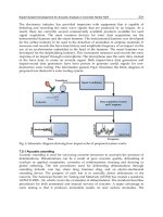
introduction. The overall structure of the proposed scheme is depicted by Figure 3.
331
An Expert System Based Approach for Diagnosis of Occurrences in Power Generating Units
6 Will-be-set-by-IN-TECH
Fig. 3. Structure of the proposed scheme.
The phasor record analysis and waveform record analysis are described in the next sections.
4. Phasor record analysis
The phasor analysis is started when a new disturbance record is available at the analysis

center. The phasor record along with the SOE are then analyzed by the proposed scheme.
The disturbance record and SOE data are read from the DFR and SCADA databases available
at the utilite’s office. Only the SOE recorded during the disturbance record time lapse is used.
Fig. 4 shows the structure of the proposed scheme. The disturbance record is firstly
preprocessed and segmented into pre- and post-disturbance parts. For each of these parts
the mean values are calculated composing the feature set used by the decision making expert
system.
Fig. 4. Structure of the proposed phasor analysis scheme.
The decision making process is made by three expert systems: ESOSC uses the features
calculated from the disturbance record to achieve a result concerning the DFR data; ESSOE
uses the sequence of events to obtain a complementary result and ESUNI correlates the results
332
Expert Systems for Human, Materials and Automation
An Expert System Based Approach for Diagnosis of Occurrences in Power Generating Units 7
from both expert systems. All the messages and conclusions achieved during the decision
making process are included in the phasor record analysis report.
The following subsections give an overview of the functional blocks of Fig. 4. A detailed
description of each block can be found in (Moreto & Rolim, 2011).
4.1 Segmentation and feature extraction
The segmentation and feature extraction process is represented by the block diagram in
Fig. 5 where indexes ABC and 012 denote the three electrical phases and three symmetrical
components (zero, positive and negative) respectively. The operator
(
|
.
|
)
is the absolute value
and
(.) represents a vector quantity.

Initial
calculation
3 power:j
P, Q, S
Segmentation
Feature
set

V
A
,

V
B
,

V
C

I
A
,

I
B
,

I
C





V
0



,




V
1



,




V
2








I
0



,




I
1



,




I
2



Fig. 5. Segmentation and feature extraction.
The recorded quantities are initially normalized to per unit (pu) values followed by the
calculation of the symmetrical components (Grainger & Stevenson, 1994) and complex power.

The segmentation process is applied to these calculated quantities in order perform a feature
extraction in each segment. The signals are split into parts before and after the transient.
In (Moreto & Rolim, 2008), the authors propose a detection index that is suitable to segment
phasor records that contain slower disturbances as observed in large power generators. This
index is calculated using Equation 1.
di
(n)=σ
Δ
(n)=
1
Δ −1
n+Δ
∑
i=n
(|

y(i)
|
−μ
Δ
)
2
(1)
Where n is the sample index,
|

y(i)
|
is the absolute value of the considered phasor quantity at
sample i, Δ is the window width, σ

Δ
is the standard deviation calculated over this window
and μ
Δ
is the mean value of the data window. In this chapter, the chosen Δ was 480 samples
(8 seconds).
When di
(n) exceeds a certain threshold δ,pointn belongs to a disturbance segment.
Consequently the first point where di
(n) > δ indicates the beginning of a disturbance interval
which ends after the last point where di
(n) > δ.
Fig. 6 presents an example of the segmentation process. The magnitude of the voltage phasor
record is segmented according to the gray bar. The calculated detection index is also shown
in the picture.
The mean value of the samples before and after the detected disturbance interval are stored in
the ESOSC facts data base.
4.2 ESOSC: Expert system for oscillographic analysis
This expert system is responsible for analyzing the data provided by the segmentation
procedure. Based on the pre- and post-disturbance data, ESOSC can classify the long term
oscillographic record in several categories.
ESOSC is represented by the diagram in Fig. 7. It is composed of 19 rules that will be described
in the following paragraphs.
333
An Expert System Based Approach for Diagnosis of Occurrences in Power Generating Units
8 Will-be-set-by-IN-TECH
Transf.
tag9
tag3
tag8

Kalman
Filter
tag4
Segments
identification
tag6
tag7
Segments
intervals
Indexes
tag5
Windowing
tag10
tag11




V
1



di
( n)
Fig. 6. Example of data segmentation and proposed detection index.
Fig. 7. ESOSC representation.
The ESOSC implementation is based on the CLIPS expert system shell with the facts being
created using CLIPS’ template objects. Each input fact contains three slots:
• Name: String with the processed quantity, such as I

0
, I
1
, I
2
, V
0
, V
1
, V
2
or P.
• PreValue: Mean value of the named quantity calculated over the pre-disturbance segment.
• PostValue: Mean value of the named quantity calculated over the post-disturbance
segment.
The ESOSC knowledge base is composed of two sets of rules. The set called Characteristics
identification rules uses the input facts as premises. According to the pre-disturbance and
post-disturbance values of each quantity, these rules create a new type of fact called
Characteristic fact which stores information about the characteristic identified in each quantity.
334
Expert Systems for Human, Materials and Automation
An Expert System Based Approach for Diagnosis of Occurrences in Power Generating Units 9
Table 1 shows the premises of each characteristics identification rule and the type characteristic
fact obtained (conclusion of the rule).
Each row of Table 1 corresponds to a rule. Some of these rules have a third premise about the
difference between the pre- and post-disturbance values of the quantity being evaluated.
Rule conclusion Pre [pu] Post [pu] Additional premise
Step-up from 0 < 0.05 > 0.05
Step-down to 0 > 0.05 < 0.05
Step-up > 0.05 > 0.05 (Post −Pre) ≥ 0.1pu

Step-down
> 0.05 > 0.05 (Pre −Post) ≥ 0.1pu
No variation
abs(Pre − Post) ≤ 0.1pu
Table 1. ESOSC: Premises and conclusions of characteristics identification rules
Depending on the values of the pre- and post-disturbance segments of a quantity one of the
rules in Table 1 is fired and a new characteristic fact is created. These facts are composed by the
following information slots:
• Name: String with the processed quantity, such as I0, I1, I2, V0, V1, V2 or P.
• Type: A string indicating the characteristic type. The values can be: Step-up from 0,
Step-down to 0, Step-up, Step-down and No variation.
• Value: The value associated with each characteristic. Normally the difference between the
pre and post-segments mean values. In the case of the No variation rule,thisvalueisthe
post-disturbance mean value.
Another set of rules was created to reason about the Charateristic facts. These rules correlate
the characteristics identified in different quantities for example, between positive sequence
voltages and currents. They also provide a conclusion about the disturbance generating a
Result fact. Table 2 shows the premises of each rule of this set which is called Characteristic
relation rules. The logical operators used to associate multiple premises are also indicated.
The rules in Table 2 conclude about the occurrence based on the disturbance record. In
some cases the oscillographic record is not enough to obtain a definitive conclusion (Moreto
& Rolim, 2011) and the SOE can be used to complement the result. The SOE analysis is
performed by the Expert System for SOE analysis (ESSOE).
4.3 ESSOE: Expert system for SOE analysis
ESSOE has two objectives: the first is to complement the ESOSC analysis (when it is
inconclusive) and the second is to provide an independent analysis, which is confronted with
the ESOSC.
Prior to the execution of the ESSOE, the sequence of events recorded during the oscillography
time lapse is selected. This selection is then classified and stored in a structured way as shown
in Fig. 8.

The events which refer to the generation unit under analysis are picked up from the SCADA
database and classified according to the four classes of Fig. 8:
• Protection Relays: The tripping events of protective relays are in this class. For each event
the data read are time stamp of the event (date and hour with millisecond precision), state
of the event (operated or normal), a code indicating the function of the relay according to
the ANSI classification and a description of the event. Usually, when the protection device
returns to its normal state another event is generated.
335
An Expert System Based Approach for Diagnosis of Occurrences in Power Generating Units
10 Will-be-set-by-IN-TECH
Rule Quantity
Characteristic type Characteristic value
Energization
and

V
+
Step-up from 0 > 0.9pu
or

I
+
Step-up from 0
I
+
No variation < 0.05pu
De-energization and

V
+

Step-down to 0 or
step-down
> 0.8pu
or

I
+
No variation < 0.05pu
P
No variation < 0.1pu
Isolated unit
and

V
+
No variation > 0.9pu
I
+
No variation < 0.05pu
Synchronism
and

V
+
No variation > 0.9pu
I
+
Step-up from 0
Normal
operation

and

V
+
No variation > 0.9pu
I
+
No variation > 0.05pu
Out of service V
+
No variation < 0.05pu
Forced
shutdown
and

V
+
Step-down to 0
I
+
Step-down to 0
P
Step-down to 0
Load
increment
and

V
+
No variation > 0.9pu

or

I
+
Step-up
P
Step-up
Load
decrement
and

V
+
No variation > 0.9pu
or

I
+
Step-down
P
Step-down
Table 2. ESOSC: Premises and conclusions of characteristics relation rules
Generation Unit
Protection Relays
Auxiliary Relays
Alarms
Circuit Breaker operation
Time stamp: {year/month/day hour:min:sec:msec}
State: {operated, normal}
Function code: {51G, 87G, }

Description: {Overcurrent relay }
Time stamp: {year/month/day hour:min:sec:msec}
State: {open, close}
Designator: {CB1, CB2, }
Description: {Main circuit breaker }
Type: {manual command, protection command}
Same fields as protection relays
Same fields as protection relays
Fig. 8. Structure of sequence of events data.
• Auxiliary Relays: This class is used to represent the auxiliary relays, such as lockout relay
(86), circuit breaker opening relay (94) and any other auxiliary device. The information
fields are the same as the protection relays class.
• Alarms: All the events that are only informative (they do not represent any protective
action) are grouped in this class.
336
Expert Systems for Human, Materials and Automation
An Expert System Based Approach for Diagnosis of Occurrences in Power Generating Units 11
• Circuit Breaker operation: This represents the events of opening and closing Circuit
Breakers (CB).
Among these classes each event is classified according to its function for instance, overcurrent
relay (ANSI 51), lockout relay (ANSI 86), main circuit breaker, manual opening of the circuit
breaker and several other functions. The classification of the events is carried out performing
a previous configuration of the system where the user informs the associations of SCADA
monitored events with the classes.
Fig. 9 shows a representation of the sequence of event analysis that is based on the ESSOE
whose input facts are the classified events and their status read from SOE database.
Input
facts
Inference
Engine

facts
Result
classification
Event
Name
Class
Type
State
SOE
rulebase
ESSOE
Fig. 9. ESSOE representation.
The knowledge base is formed by a set of rules obtained from the protection scheme of
every generation unit with the collaboration of protection specialists. It is necessary to
know which protective devices trip the circuit breakers, which ones are the auxiliary relays
and their actions, the energization and de-energization procedures of the unit and other
relevant characteristics or procedures associated with each generation unit. From these
studies it is possible to write several rules. The ESSOE has 8 rules for the following
situations: de-energization, reverse power de-energization, isolated unit de-energization, protection
testing (maintenance), generator lockout, synchronization of unit, forced shutdown and the no
events. (Moreto & Rolim, 2011).
The SOE analysis and oscillographic analysis should be correlated in order to obtain a final
conclusion about the occurrence (Moreto & Rolim, 2011). This is the objective of the Expert
System for generation Unit analysis (ESUNI).
4.4 ESUNI: Expert System for Unit analysis
The ESUNI is responsible for correlating the results from oscillograph (ESOSC) and sequence
of events (ESSOE) analysis providing a diagnosis about the generation unit. It consists of
an expert system with a set of simple rules that compares each result. These rules, listed in
Table 3, represent a set of possible final results from the phasor record and sequence of events
analyses (Moreto & Rolim, 2011).

A “no result” is obtained when none of the Table 3 rules is satisfied. The most common causes
of “no result” conclusion are:
• Failures in the data collection system, such as missing events in the SOE
• Synchronization failure between the oscillographic records and the SOE
• Spurious events in SOE due to noise at RTU inputs
• Wrong connections of current or voltage transformers with the DFR
When the conclusion is “no result” or “fault”, a subsequent analysis is needed, using the
waveform record in order to detect and classify possible faults.
337
An Expert System Based Approach for Diagnosis of Occurrences in Power Generating Units
12 Will-be-set-by-IN-TECH
ESUNI conclusion ESOSC ESSOE
Normal operation
Normal operation No events
Load increment No events
Load decrement No events
Out of service Out of service No events
Reverse power de-energization De-energization De-energization with 32G
Normal de-energization De-energization De-energization
Energization
Energization Generator lock-out
Energization Synchronism
Protection system tests Out of service Protection testing
Isolated unit operation Isolated unit No events
Synchronism
Synchronism Synchronism
Isolated unit Synchronism
Normal operation Synchronism
Fault or forced shutdown Forced shutdown Forced shutdown
Table 3. ESUNI rule set.

5. Waveform record analysis
The structure of the waveform record analysis scheme is composed by the following
processing blocks that are executed in sequence (Fig. 10): Data acquisition; data segmentation;
data feature extraction; and decision making (expert system based).
Fig. 10. Processing blocks of the waveform analysis scheme.
Data acquisition is the process of reading and interpreting the data stored in DFR records.
These data are the sampled waveforms of voltages and currents acquired at the generator
terminals. The segmentation block is responsible for detecting transients in the acquired data,
resulting in a set of pre-fault, fault and post-fault segments. An Extended Complex Kalman
Filter (ECKF) is used for this purpose (Nishiyama, 1997). For each detected segment a feature
extraction is performed and those features will be used as inputs to the decision making
process. Parameters of the signal estimated by the ECKF and also by linear Kalman Filters
(KF) are used to calculate the input features of the expert system.
The occurrence analysis based on the DFR waveform records is also performed by an expert
system. The input facts are the calculated features and the output fact is the type of
disturbance. Development of the rule set was made based on several simulations of a power
generating unit bay composed a hydraulic turbine, a synchronous machine, a speed regulator,
a voltage regulator and a step-up transformer. In the simulated system this unit is connected
to an slack bus which represents a bulk power system.
The processing blocks of Fig. 10 will be discussed in detail in the following subsections.
5.1 Data segmentation
Segmentation consists of splitting a disturbance record that is not stationary into a series of
segments that can be considered stationary (Bollen & Gu, 2006). Through a segmentation
process, traditional tools like Fourier analysis can be applied to each segment without the
338
Expert Systems for Human, Materials and Automation
An Expert System Based Approach for Diagnosis of Occurrences in Power Generating Units 13
errors that would occur when such tools are employed in non-stationary signals. An example
of segmentation is shown in Fig. 11.
Fig. 11. Exemple of waveform record segmentation.

Several signal processing tools can be employed in the segmentation process. The most
common ones are the Short Time Fourier Transform (STFT) (Gu & Bollen, 2000), the Wavelet
Transform (Silva et al., 2006; Ukil & Zivanovic, 2007) and adaptive filters like Kalman Filters
(Bollen & Gu, 2006; Styvaktakis et al., 2002). The segmentation schemes proposed in the
literature are not appropriate for power generation units, because they have not been designed
for segmenting slow transients like the example of Fig. 2(b). To overcome this limitation a
new segmentation scheme is proposed in this chapter. This scheme is based on an extended
complex Kalman filter (ECKF). Before the explanation of the signal model used and the
segmentation algorithm, a brief introdution to Kalman filters is presented.
5.1.1 Kalman filters
The Kalman filter (KF) is a recursive and efficient estimation process that minimizes the mean
square error of a signal model based on measured values. The process uses a observation
variable obtained from the measurements (DFR data) to estimate the state variables. In its
basic formulation, the relation between the states and the measurements and the relation
between the actual states and previous ones are assumed to be linear. This implies that the
model to be estimated can be written as state variables where all Matrix elements are constants
(Bollen & Gu, 2006):
State equations: x
k+1
= Φ
k
x
k
+ w
k
(2)
Observation equations: y
k
= H
k

x
k
+ v
k
(3)
where x
k
is the state vector at instant k; Φ
k
is the state transition matrix that provides the
relation between instants k and k
+ 1andH
k
is the observation matrix that relates the states
with the measurements y
k
. w
k
and v
k
are vectors representing the noise of the model and the
measurements respectively. It is assumed that both are white noise, non correlated, with zero
mean and covariance matrix Q
k
= E

w
k
w
T

k

and R
k
= E

v
k
v
T
k

where E is the expected
value operation.
The recursive calculation of the Kalman filter starts from an initial estimation of the state
vector ˆx
0
and the error covariance matrix
ˆ
P
0
. With these values the Kalman gain K
k
is
calculated for sample k:
K
k
=
ˆ
P

k−1
H
∗T
k

H
k
ˆ
P
k−1
H
∗T
k
+ R

−1
(4)
where the operations denoted by
∗
e
T
are the complex conjugate and transposition,
respectively. R is the covariance of the measurement noise, assumed constant and acts as
a speed adjustment parameter of the filter.
339
An Expert System Based Approach for Diagnosis of Occurrences in Power Generating Units
14 Will-be-set-by-IN-TECH
With the updated gain, the covariance matrix is also updated,
ˆ
P

k
=
ˆ
P
k−1
(
I −K
k
H
k
)
(5)
as well for state vector, using the new measurement y
k
to correct it:
ˆx
k
= ˆx
k−1
+ K
k
(
y
k
− H
k
ˆx
k−1
)
(6)

The term between parenthesis in Equation 6 is called innovation or residual. I is the identity
matrix.
Finally a projection of the states and covariance matrix is calculated:
x
k+1
= Φ
k
x
k
(7)
ˆ
P
k+1
= Φ
k
ˆ
P
k
Φ
∗T
k
(8)
With the projected values, the k index is incremented and a new iteration begins with the
application of Equation 4. The process continues until k
= N,whereN is the total number of
samples.
If the relations of the state equations and observation equations are non-linear, the extended
Kalman filter (EKF) is more adequate. In EKF the matrix operations of Equations 2 and 3 are
replaced by nonlinear functions:
x

k+1
= φ
k
(
x
k
)
+
w
k
(9)
y
k
= h
k
(
x
k
)
+
v
k
(10)
To apply the EKF, the non-linear model (Equations 9) and the output equation (Equation 10)
are linearized using the first term of the Taylor series. As a result, Equations 4, 5, 6 and 8
become (Girgis & Hwang, 1984):
Φ
k
=
∂φ

k
(
x
k
)
∂x
k




x
k
=ˆx
k
(11)
H
k
=
∂h
k
(
x
k
)
∂x
k





x
k
=ˆx
k−1
(12)
5.1.2 Signal model
In this chapter the parameters of the signal model are estimated by a extended Kalman filter.
The proposed model, expressed in Equations 13 to 15 is a complex sinusoid with a damping
coefficient:
y
k
= z
k
+ v
k
(13)
where:
z
k
= e
λt
k
A
1
e
j
(
ω
1

t
k
+ϕ
i
)
(14)
ω
1
= 2π f
1
, t
k
= kΔt (15)
The term A
1
represents the sinusoid magnitude, ϕ
i
the phase angle and f
1
the system’s
fundamental frequency (usually 50Hz or 60Hz). The exponential damping coefficient is given
by λ,andΔt is the sampling period.
340
Expert Systems for Human, Materials and Automation
An Expert System Based Approach for Diagnosis of Occurrences in Power Generating Units 15
This model can be written in state variable form (Nishiyama, 1997):

x
k+1
(1)

x
k+1
(2)

=

10
0 x
k
(1)

x
k
(1)
x
k
(2)

(16)
y
k
=

01


x
k
(1)
x

k
(2)

+ v
k
(17)
where:
x
k
(1)=e
λΔt+jω
1
Δt
(18)
x
k
(2)=A
1
e
λkΔt+j
(
ω
1
kΔt+ϕ
1
)
= z
k
(19)
As the model is non-linear, the equations of the EKF have to be used. It should be pointed out

that the measured signals are complex quantities, obtained from the three phase components
using the αβ transform as in (Dash et al., 1999; Hase, 2007).
With the estimated states it is possible to estimate of the fundamental frequency (
ˆ
f
1k
),
exponential damping coefficient (
ˆ
λ
k
), fundamental component magnitude (
ˆ
A
1k
)andphase
angle (
ˆ
ϕ
1k
) using the following relations:
ˆ
f
1k
=
ω
1k
2π
=
1

2πΔt
Imag
(
ln
(
ˆ
x
k
(1)
))
(20)
ˆ
λ
k
=
1
Δt
Real
(
ln
(
ˆ
x
k
(1)
))
(21)
ˆ
A
1k

=
|
ˆ
x
k
(2)
|
(22)
ˆ
ϕ
1k
= Imag

ˆ
x
k
(2)
|
ˆ
x
k
(2)
|
ˆ
x
k
(1)
k

(23)

5.1.3 Segmentation algor ithm
The overall scheme of the proposed segmentation algorithm is shown in Fig. 12.
Transf.
Kalman
Filter
Segments
identification
Segments
indexes
Indexes
Windowing
y
ka
y
kb
y
kc
y
k
ˆ
λ
k
σ
λk
> limiar
limiar
Δ
idx
αβ
std

(
ˆ
λ
k
)=σ
λk
Δ
std
Fig. 12. Proposed segmentation scheme.
Each block in Fig. 12 is described in the following paragraphs:
5.1.3.1 ① Complex signal calculation
The measured complex signal y
k
is obtained from the three phase measurements contained in
the disturbance record (y
ka
, y
kb
and y
kc
)usingtheαβ transform (Hase, 2007) of Equations 24
and 25.
341
An Expert System Based Approach for Diagnosis of Occurrences in Power Generating Units
16 Will-be-set-by-IN-TECH

y
kα
y
kβ


=

2
3

1
−
1
2
−
1
2
0
√
3
2
−
√
3
2

⎡
⎣
y
ka
y
kb
y
kc

⎤
⎦
(24)
y
k
= y
kα
+ jy
kβ
(25)
5.1.3.2 ②Kalman filter calculation
The extended complex Kalman filter is applied to y
k
and the parameter
ˆ
λ
k
is estimated. This
signal is used to segment the disturbance record.
5.1.3.3 ③Detection index calculation
The signal
ˆ
λ
k
is submitted to a windowing procedure where at each window of length Δ
std
the standard deviation is calculated. The result of the sliding windows calculations is the
detection index σ
λk
, similar to the detection index applied for the phasor record segmentation.

5.1.3.4 ④Threshold comparison
A new segment is identified as the period when the detection index exceeds a given threshold.
Thus, the threshold detection gives the beginning and the ending of the segments.
5.1.3.5 ⑤Segments identification
The segments identified at the previous step are analyzed in such a way that those considered
close enough are grouped in a single segment. The parameter Δ
idx
correspond to the
minimum time interval between two consecutive segments. The time instants of the beginning
and ending of each segment are used to calculate the features that will be used by the expert
system.
5.2 Feature extracti on
The process of feature extraction is based on the fundamental frequency phasors of each
monitored quantity, obtained through a set of linear Kalman filters. The signal model
used is the number 1 of (Kennedy et al., 2003). From these calculated phasor parameters,
the symmetrical components are calculated. Finally, a mean value of each symmetrical
component magnitude is calculated in each segment. This process is depicted in Fig. 13.
The inputs are the voltages (V
A
, V
B
and V
C
)andcurrents(I
A
, I
B
and I
C
) at the terminals of

the generator and the neutral current at the high side of the unit’s step-up transformer (I
nHS
).
These quantities are usually monitored by the DFRs at power stations.
5.3 Decision making
An expert system is the core of the waveform analysis. This tool is suitable to this application,
due to its ability to represent the knowledge applied by the specialist to solve the problem.
The facts knowledge base of this expert system is composed of facts containing the calculated
quantities stated in the previous subsection for each segment identified. The fields that
compose these facts are described in Table 4.
The fields “Disturb.” and “Classific.” are used during the reasoning process to store the results
of the analysis. That is, their content shows the classification of each disturbance segment.
By defining the facts structure, the rule base can be described. These rules can be grouped in
sets to facilitate the explanation process, but they coexist simultaneously at the expert system
knowledge base. The defined sets are:
342
Expert Systems for Human, Materials and Automation
An Expert System Based Approach for Diagnosis of Occurrences in Power Generating Units 17
Fig. 13. Feature extraction process.
Field or slot Description
Num Number of the segments
V0m Mean value of the zero sequence voltage modulus
V1m Mean value of the positive sequence voltage modulus
V2m Mean value of the negative sequence voltage modulus
I0m Mean value of the zero sequence current modulus
I1m Mean value of the positive sequence current modulus
I2m Mean value of the negative sequence current modulus
InATm Mean value of the high side neutral current modulus
CexpVm
Mean value of the damping coeficient

ˆ
λ
k
ModV12m
Mean value of

V1 −

V2 modulus
Disturb. Type of identified disturbance
Classific. Classification of the disturbance
Table 4. Fact contents of the waveform analysis expert system.
• Fault detection rules.
• Classification of normal situations rules.
• Fault classification rules.
Each rule set is described below.
5.3.1 Fault detection rules
The objective of this set of rules is to determine if a segment shows characteristics of a short
circuit (balanced or unbalanced) or represents a normal operative situation. These rules are
343
An Expert System Based Approach for Diagnosis of Occurrences in Power Generating Units
18 Will-be-set-by-IN-TECH
mainly based on the values of negative sequence voltages and currents, which indicate an
imbalance between the three phases.
The conclusion of the rules is the fulfillment of the field “Disturb.” with a corresponding code.
When rule-based expert systems are build in CLIPS platform, this modification is equivalent
to the redefinition of the fact in the knowledge base.
Table 5 summarizes de fault detection rules. The symbol
⇐ is used to denote a field
modification within in the fact. The premises column shows the thresholds used to detect

each type of disturbance and also the logical operators “and” and “or”.
Rule conclusion Action Premises
Normal operation Disturb.⇐“normal”
V2m < 0.1pu and
I2m
< 0.07pu and
I1m
< 1.1pu
Unbalanced fault Disturb.⇐“unbalanced”
V2m > 0.1pu or
I2m
> 0.07pu
Balanced fault Disturb.⇐“balanced”
V2m < 0.1pu or
I2m
< 0.07pu and
I1m
> 1.1pu
Table 5. Premises of fault detection rules.
5.3.2 Classificati on of normal sit uation rules
These rules are responsible for classifying the segment were “normal” operative situation
have been detected in, for instance: de-energization, normal operation, generator unloaded,
generator shutdown and so on. The rules for classifying normal situations are presented in
Table 6.
Rule conclusion Action Premises
Normal operation with
load
Classifi.⇐“normal load”
V1m > 0.9pu and
I1m

> 0.05pu and
Disturb. = “normal”
Normal operation
without load
Classifi.⇐“normal no load”
V1m > 0.9pu and
I1m
< 0.05pu and
Disturb. = “normal”
Shutdown Classifi.⇐“shutdown”
V1m < 0.1pu and
I1m
< 0.05pu and
Disturb. = “normal”
De-energization Classifi.⇐“De-energization”
0.1 <V1m< 0.9pu and
I1m
< 0.05pu and
CexpVm
< −0.2 and
Disturb. = “normal”
Table 6. Premises and actions of the rules to classify normal situations.
In this rule set, the premises are based on the positive sequence values, but they will not fire if
an acceptable imbalance or overload situation is detected as a Disturb. = “normal” condition is
needed. The classified operative conditions are: normal operation with load (nominal voltage
and current), normal operation without load (nominal voltage and no current), generator
shutdown (no voltages and currents) and de-enegization (voltage at intermediate levels with
exponential decrease and no current).
344
Expert Systems for Human, Materials and Automation

An Expert System Based Approach for Diagnosis of Occurrences in Power Generating Units 19
5.3.3 Fault classification rules
These rules a used to classify those cases when an imbalance condition is detected. Their
premised are based on the relations between the symmetrical components values obtained by
short circuit analysis theory (Grainger & Stevenson, 1994). These relations are stated below
for two phase faults.

I1 ≈−

I2 (26)

V1 ≈

V2 (27)

V0 ≈

I0 ≈ 0 (28)
Concerning two phase to ground faults, the relations are the following:

I1 ≈−

I2 −

I0 (29)

V1 ≈

V2 ≈


V0 (30)
And for single phase to ground:

I1 ≈

I2 ≈

I0 (31)

V1 ≈

V2 +

V0 ⇒−

V1 +

V2 +

V0 ≈ 0 (32)
The relations mentioned are valid in the faulted point of the system. If a fault occurs in the
nearby system (like in the power plant substation), they will be influenced by the distance to
the fault and by the connections of the power transformer. Most of the step-up transformers
employed in generation units have Δ-Y configuration. This way, a single phase to ground fault
at the transformer high voltage side is “seen” as a two phase fault at the generator terminals.
In order to discriminate ground faults and phase faults at the transformer high voltage side
the neutral current I
nHS
is used. The presence of this current indicates a ground fault in the
high voltage side. Table 7 shows the set of rules used to classify the disturbances.

The classification of each segment, along with the messages generated by each rule, are stored
sequentially (using the same order of the segments) in the waveform analysis report. In the
event of a fault, the analysis conclusion is its classification otherwise it is the normal operation
classification. The expert engineer can then check the report where all the information needed
is condensed, which result in less time spent and an improvement of the quality of the
analysis.
6. Results
The approach explained in the previous section, has been tested using real data from a coal
fired thermal power plant in Brazil. This power plant has four 24 MVA turbogenerators. The
DFR monitors the terminal voltages and load currents from the four turbogenerators (G1 to
G4).
The scheme is implemented as a standalone application written in python language. The
expert systems have been implemented in CLIPS and interfaced with the routines in python.
Some results of phasor and waveform record automatic analyses are presented in the
following subsections.
345
An Expert System Based Approach for Diagnosis of Occurrences in Power Generating Units