Heat and Mass Transfer Modeling and Simulation Part 6 pptx
Bạn đang xem bản rút gọn của tài liệu. Xem và tải ngay bản đầy đủ của tài liệu tại đây (802.46 KB, 20 trang )
Process Intensification of Steam Reforming for Hydrogen Production
91
Optimum conditions of the reactor were obtained. Hydrogen yield reached
0.2 mol/(h·g
cat
) under condition of T
r
=260 ℃, W/M=1.3 and WGHV=0.2 h
-1
, which can
provide hydrogen for 10.2W PEMFC with a hydrogen utilization of 80% and an fuel
cell efficiency of 60%. A 3-D model coupling with parallel reaction kinetics was
obtained by data fitting to describe its performance. Furthermore, gradually
increased catalyst activity in the reaction channel can be used to further reduce the
cold spot effect; Hydrogen content at reactor outlet increased by about 8.5%
compared with catalyst uniform distribution condition; while outlet CO content
reduced to less than 0.13%.
2.
Cold spray technology was successfully used to catalytic coatings fabrication for fuel
reforming reaction and all the powers were effectively deposited onto the substrates.
Components of the coatings were approximately identical to the initial powders.
Performance of the coating was influenced by impact velocity and broken character of
the particles especially for the NiO/Al
2
O
3
and CuO/ZnO/Al
2
O
3
catalytic coatings.
For the Cu coating, carbon deposition is serious which resulted in nonstable activity
in methanol steam reforming compared with Cu-Al
2
O
3
coating. At condition of inlet
temperature 265
℃, W/M of 1.3, space velocity of 162h
-1
, H
2
content in the products
for CuO/ZnO/Al
2
O
3
catalytic coating reaches 52.3%, whereas CO content is only
0.60%. Methane primary steam reforming on cold sprayed NiO/Al
2
O
3
coating also
indicated a superior character to kernel catalyst in packed bed reactor as its high
output.
3.
Through interrupted distribution of catalytic surface, at same conditions methanol
conversion could be improved although the temperature in reaction channel became
uneven. So in micro-reactors which utilize coating catalyst, this interrupted distribution
of surface can improve the efficiency of catalyst and thus reduce loading and cost of
reforming catalyst. The optimal activity distribution was that the activity should be low
at inlet, along with the reactor channel, the activity gradually increased. This kind of
activity distribution can also be used to decrease the cold spot temperature difference in
the reactor. The 3-D simulation results of MSR for hydrogen production in self-
designed plate micro reactor showed that micro-reactors can maintain a high hydrogen
molar fraction and methanol conversion at high reactant flow rate. It is also reasonable
to integrate all reaction units in fuel reforming system in one channel to mach up
PEMFC for CO requirement.
Therefore, through the adoption of both micro-scale reactors and coating catalyst, heat and
mass transfer in the reaction channel for hydrogen production by fuel reforming can be
enhanced resulting in the improvement of reactor performance. Nowadays, research of
process intensification by the above methods becomes more and more, and it is beneficial
for the development of hydrogen production through hydrocarbon fuel reforming
technology. All the endeavors will promote the application of hydrogen energy. We look
forward to the day of hydrogen economy coming soon.
7. Acknowledgements
The authors acknowledge the support of National Natural Science Foundation of China
(50906104) and project No.CDJZR10140010 supported by Fundamental Research Funds for
the Central Universities.
Heat and Mass Transfer – Modeling and Simulation
92
8. Nomenclature
C
molar concentration, kmol/m
3
P
mixed gas pressure, Pa
p
C
Isobaric specific heat capacity,
J/(mol·K)
mixed gas viscosity coefficient,
kg/(m·s)
D
effective diffusion coefficient, m
2
/s or
thickness, mm; or catal
y
st and catal
y
tic
coating distribution types
T , T
r
mixed gas temperature and
reaction temperature, K or
℃
mixed gas density, kg/m
3
L
Channel length or channel
subsection length, mm
V , v
mixed gas velocity, m/s
M
molar mass, kg/mol
Y
, F
component molar fraction, %
m
mass fraction, %
V
mixed gas velocity, m/s or rate of inlet
liquid flow, ml/min
S
selectivity, %
q
,
q
heat of reaction, W/m
2
S/M,
W/M
water methanol ratio
R
, r ,
a
reaction rate, mol/(g
cat
h) E
a
activation energy, kJ/mol
'
r
reaction rate, kmol/(m
2
s)
h
height of channel, mm or specific
enthalphy, J/kg
R
universal gas constant, kJ/(molK) H height of channel, mm
H
0
standard enthalpy of formation, J/kg
X
conversion, %
k
reaction rate constant, mol/(kg
cat
s) WHSV liquid space velocity, h
-1
K
reaction equilibrium constant
0
k ,
'
0
k
frequency factor, mol/(kg
cat
s)
a, b thickness, mm
up,
down
mark of up and down channel
n
number of interruption or activity
exponential doubling number
W/F
ratio of mole flow rate and catalyst
weight, g·h/mol
Subscript:
0, in inlet parameters out outlet parameters
1, 2
mark of channel or catalyst coating
subsection
s=1~5
reactants and products of CH
3
OH,
H
2
O, H
2
, CO, CO
2
i
mark of channel or catalyst coating
subsection
(CH
3
OH) represent of methanol parameter
w reaction channel wall (CO
2
) represent of CO
2
parameter
cat. represent of catalyst parameter (H
2
) represent of H
2
parameter
(F) molar fraction (H
2
O) represent of H
2
O parameter
WGS water gas shift reaction (CO) represent of CO parameter
SR steam reforming reaction O
2
represent of O
2
parameter
DE methanol decomposition
△
variable difference
RWGS reverse water gas shift reaction (X) represent of conversion
Process Intensification of Steam Reforming for Hydrogen Production
93
9. References
[1] Carl-Jochen Winter. (2009). Hydrogen energy — Abundant, efficient, clean: A debate
over the energy-system-of-change.
International Journal of Hydrogen Energy, Vol. 34,
No. 14, Supplement 1, (July 2009), pp. (S1-S52), 0360-3199
[2] Anand S. Joshi, Ibrahim Dincer, Bale V. Reddy. (2010). Exergetic assessment of solar
hydrogen production methods.
International Journal of Hydrogen Energy, Vol. 35, No.
10, (May 2010), pp. (4901-4908), 0360-3199
[3] Jianlong Wang, Wei Wan. (2009). Experimental design methods for fermentative
hydrogen production: A review.
International Journal of Hydrogen Energy, Vol. 34,
No. 1, (January 2009), pp. (235-244), 0360-3199
[4] Michael G. Beaver, Hugo S. Caram, Shivaji Sircar. (2010). Sorption enhanced reaction
process for direct production of fuel-cell grade hydrogen by low temperature
catalytic steam–methane reforming.
Journal of Power Sources, Vol. 195, No. 7, 2,
(April 2010), pp. (1998-2002), 0378-7753
[5] Guangming Zeng, Ye Tian, Yongdan Li. (2010). Thermodynamic analysis of hydrogen
production for fuel cell via oxidative steam reforming of propane.
International
Journal of Hydrogen Energy
, Vol. 35, No. 13, (July 2010), pp. (6726-6737), 0360-3199
[6] Stefan Martin, Antje Wörner. (2011). On-board reforming of biodiesel and bioethanol for
high temperature PEM fuel cells: Comparison of autothermal reforming and steam
reforming.
Journal of Power Sources, Vol. 196, No. 6, 15, (March 2011), pp. (3163-
3171), 0378-7753
[7] Feng Wang, Dingwen Zhang, Shiwei Zheng, Bo Qi. (2010). Characteristic of cold sprayed
catalytic coating for hydrogen production through fuel reforming.
International
Journal of Hydrogen Energy
, Vol. 35, No. 15, (August 2010), pp. (8206-8215), 0360-
3199
[8] M. H. Akbari, A. H. Sharafian Ardakani, M. Andisheh Tadbir. (2011). A microreactor
modeling, analysis and optimization for methane autothermal reforming in fuel cell
applications.
Chemical Engineering Journal, Vol. 166, No. 3, 1 (February 2011), pp.
(1116-1125), 1385-8947
[9] Akira Nishimura, Nobuyuki Komatsu, Go Mitsui, Masafumi Hirota, Eric Hu. (2009). CO
2
reforming into fuel using TiO
2
photocatalyst and gas separation membrane.
Catalysis Today, Vol. 148, No. 3-4, 30 (November 2009), pp. (341-349), 0920-5861
[10] Feng Wang, Longjian Li, Bo Qi, Wenzhi Cui, Mingdao Xin, Qinghua Chen, Lianfeng
Deng. (2008). Methanol steam reforming for hydrogen production in a minireactor.
Journal of Xi ’An J iao Tong University
, Vol. 42, No. 4, (April 2008), pp. (341-349), 509-
514, 0253-987X
[11] Feng Wang, Jing Zhou, Zilong An, Xinjing Zhou. (2011). Characteristic of Cu-based
catalytic coating for methanol steam reforming prepared by cold spray.
Advanced
Materials Research
, Vol. 156-157, (2011), pp. (68-73), 1022-6680
[12] H. Purnama, T. Ressler, R. E. Jentoft, H. Soerijanto, R. Schlögl, R. Schomäcker. (2004).
CO Formation / Selectivity for Steam Reforming of Methanol with a Commercial
CuO/ZnO/Al
2
O
3
Catalyst. Applied Catalysis A: General, Vol. 259, No.1, 8, (March
2004), pp. (83-94), 0926-860X
[13] Yongtaek Choi, Harvey G Stenger. (2003). Water Gas Shift Reaction Kinetics and
Reactor Modeling for Fuel Cell Grade Hydrogen.
Journal of Power Sources, Vol. 124,
No. 2, (November 2003), pp. (432-439), 0378-7753
Heat and Mass Transfer – Modeling and Simulation
94
[14] Y. H. Wang, J. L. Zhu, J. C. Zhang, L.F. Song, J. Y. Hu, S. L. Ong, W. J. Ng. (2006).
Selective Oxidation of CO in Hydrogen-rich Mixtures and Kinetics Investigation on
Platinum-gold Supported on Zinc Oxide Catalyst.
Journal of Power Sources, Vol. 155,
No. 2, (April 2006), pp. (440-446), 0378-7753
5
Heat and Mass Transfer in External
Boundary Layer Flows Using Nanofluids
Catalin Popa, Guillaume Polidori, Ahlem Arfaoui and Stéphane Fohanno
Université de Reims Champagne-Ardenne, GRESPI/Thermomécanique (EA4301)
Moulin de la Housse, BP1039, 51687 Reims cedex 2,
France
1. Introduction
The application of additives to base liquids in the sole aim to increase the heat transfer
coefficient is considered as an interesting mean for thermal systems. Nanofluids, prepared
by dispersing nanometer-sized solid particles in a base-fluid (liquid), have been extensively
studied for more than a decade due to the observation of an interesting increase in thermal
conductivity compared to that of the base-fluid (Xuan & Roetzel, 2000; Xuan & Li, 2000).
Initially, research works devoted to nanofluids were mainly focussed on the way to increase
the thermal conductivity by modifying the particle volume fraction, the particle size/shape
or the base-fluid (Murshed et al., 2005; Wang & Mujumdar, 2007). Using nanofluids strongly
influences the boundary layer thickness by modifying the viscosity of the resulting mixture
leading to variations in the mass transfer in the vicinity of walls in external boundary-layer
flows. Then, research works on convective heat transfer, with nanofluids as working fluids,
have been carried out in order to test their potential for applications related to industrial
heat exchangers. It is now well known that in forced convection (Maïga et al. 2005) as well as
in mixed convection, using nanofluids can produce a considerable enhancement of the heat
transfer coefficient that increases with the increasing nanoparticle volume fraction. As
concerns natural convection, the fewer results published in the literature (Khanafer et al.
2003; Polidori et al., 2007; Popa et al., 2010; Putra et al. 2003) lead to more mixed conclusions.
For example, recent works by Polidori et al. (2007) and Popa et al. (2010) have led to
numerical results showing that the use of Newtonian nanofluids for the purpose of heat
transfer enhancement in natural convection was not obvious, as such enhancement is
dependent not only on nanofluids effective thermal conductivities but on their viscosities as
well. This means that an exact determination of the heat transfer parameters is not
warranted as long as the question of the choice of an adequate and realistic effective
viscosity model is not resolved (Polidori et al. 2007, Keblinski et al. 2008). It is worth
mentioning that this viewpoint is also confirmed in a recent work (Ben Mansour et al., 2007)
for forced convection, in which the authors indicated that the assessment of the heat transfer
enhancement potential of a nanofluid is difficult and closely dependent on the way the
nanofluid properties are modelled. Therefore, the aim of this paper is to present theoretical
models fully describing the natural and forced convective heat and mass transfer regimes
for nanofluids flowing in semi-infinite geometries, i.e. external boundary layer flows along
Heat and Mass Transfer – Modeling and Simulation
96
flat plates. In order to reach this goal, the integral formalism is extended to nanofluids. This
work is the continuation of previous studies carried out to develop free and forced
convection theories of external boundary layer flows by using the integral formalism
(Polidori et al., 1999; Polidori et al., 2000; Polidori & Padet, 2002; Polidori et al., 2003; Varga
et al., 2004) as well as to investigate convective heat and mass transfer properties of
nanofluids (Fohanno et al., 2010; Nguyen et al., 2009; Polidori et al., 2007; Popa et al., 2010)
where both viscosity and conductivity analytical models have been used and compared
with experimental data. The Brownian motion has also been taken into account.
Nevertheless these studies focused mainly heat transfer. Free and forced convection theories
have been developed both in the laminar and turbulent regimes and applied to conventional
fluids such as water and air. Application of the integral formalism to nanofluids has been
recently proposed in the case of laminar free convection (Polidori et al., 2007; Popa et al.
2010).
In order to develop these models, nanofluids will be considered flowing in the laminar
regime over a semi-infinite flat plate suddenly heated with arbitrary heat flux densities. The
laminar flow regime in forced and natural convection is investigated for Prandtl numbers
representative of nanofluids. The nanofluids considered for this study, at ambient
temperature, are water-alumina and water-CuO suspensions composed of solid alumina
nanoparticles with diameter of 47 nm (
p
=3880 kg/m
3
) and solid copper oxide nanoparticles
with diameter of 29 nm (
p
= 6500 kg/m
3
) with water as base-fluid. The thermophysical
properties of the nanofluids are obtained by using empirical models based on experimental
data for computing viscosity and thermal conductivity of water-alumina and water-CuO
suspensions, and based on a macroscopic modelling for the other properties. The influence
of the particle volume fraction is investigated in the range 0%≤≤5%.
The chapter is organized as follows. First, the development of the integral formalism
(Karman Pohlhausen approach) for both types of convection (free and forced) in the laminar
regime is provided in Section 2. Then, Section 3 details a presentation of nanofluids.
A particular attention is paid on the modelling of nanofluid thermophysical properties and
their limitations. Section 4 is devoted to the application of the theoretical models to the
study of external boundary-layer natural and forced convection flows for the two types of
nanofluids. Results are presented for particle volume fractions up to 5%. Results on the flow
dynamics are first provided in terms of velocity profiles, streamlines and boundary layer
thickness. Heat transfer characteristics are then presented by means of wall temperature
distribution and convective heat transfer coefficients.
2. Mathematical formulation
2.1 Natural convection
Consider laminar free convection along a vertical plate initially located in a quiescent fluid
under a uniform heat flux density thermal condition. Denote U and V respectively the
velocity components in the streamwise x and crosswise y directions. Assuming constant
fluid properties and negligible viscous dissipation (Boussinesq’s approximations) the
continuity, boundary-layer momentum and energy equations are:
Continuity equation:
+
=0 (1)
Heat and Mass Transfer in External Boundary Layer Flows Using Nanofluids
97
Momentum equation:
+
=
−
+
(2)
Energy equation:
+
=
(3)
Using the Karman-Pohlhausen integral method (Kakaç and Yener, 1995 ; Padet, 1997),
physically polynomial profiles of fourth order are assumed for flow velocity and
temperature across the corresponding hydrodynamic and thermal boundary layers (see
Figure 1). The major advantage in using such a method is that the resulting equations are
solved anatically.
Fig. 1. Schematization of external boundary layer flows in forced convection (left) and free
convection (right)
The method of analysis assumes that the velocity and temperature distributions have
temporal similarity (Polidori et al., 2000) meaning that the ratio between the temperature
and the velocity layers depends only upon the Prandtl number.
∆=
(4)
Thus, combining relation (4), the Fourier’s law and adequate boundary conditions leads to
the following U-velocity and temperature polynomial distributions depending mainly
upon the dynamical parameter:
Heat and Mass Transfer – Modeling and Simulation
98
=
∆
−
+3
−3
+
(5)
Θ=−
=
∆
−
+2
−2
+1 (6)
Where =
≤1,
=
≤1, β is the volumetric coefficient of thermal expansion, k is the
thermal conductivity of the fluid, is the fluid kinematic viscosity, and
w
is the heat flux
density.
With the correlation (4), the integral forms of the boundary-layer momentum and energy
conservation equations become :
=
Θ
−
(7)
Θ
=−
(8)
The analytical resolution of the system (Eq. 7 and Eq. 8) leads to the knowledge of the
boundary layer ratio (Polidori et al., 2000) and on the other hand gives the steady
evolution of the asymptotical solution.
Thus, introducing the parameter =ln
, the evolution of the ratio (Pr) is found to be
suitable whatever Pr > 0.6 and satisfactorily approached with the following relation :
∆= 1.576×10
−4.227×10
+4.282×10
−0.1961+0.901 (9)
The asymptotical limit of the dynamical boundary layer thickness is analytically expressed
as :
δ
=Ω
(10)
where
Ω=
∆
9∆−5
(11)
The best way to understand how the mass transfer occurs and how the boundary layer is
feeded with fluid is to access the paths following by the fluid from the streamline patterns.
For this purpose, let introduce a stream function (x,y) such that
= and
=
with the condition (x,0) = 0 so that the continuity equation (1) is identically satisfied. The
analytical resolution leads to the following steady state solution :
Ψ
,,→∞
=
∆
−
+
−Ω
+
(12)
Θ
=
−
=
∆
9∆−5
(13)
Newton’s law:
h=
(14)
Heat and Mass Transfer in External Boundary Layer Flows Using Nanofluids
99
2.2 Forced convection
The schematization of the forced convection physical problem is seen in Figure 1. The
mathematical approach is based on the energy semi-integral equation resolution within the
thermal boundary layer, by using the Karman-Pohlhausen method applied to both velocity
and temperature flow fields.
Θ
=−
(15)
The determination of the ratio (steady relative thickness of both thermal and dynamical
boundary layers) is made from the resolution of the steady form of the energy equation
(Padet, 1997) from which it is shown that this parameter appears to be only fluid Prandtl
number dependent. The resulting equation in the Prandtl number range covering the main
usual fluids, namely Pr > 0.6, is written as :
∆
−
∆
+
∆
−
=0
(16)
Using the 4
th
order Pohlhausen method with convenient velocity and thermal boundary
conditions leads to the following velocity and temperature profiles :
=
−2
+2
(17)
Θ=Θ
−
+2
−2
+1
(18)
These profiles are directly used to define dynamical parameters qualifying both heat and
mass transfer, such as the dynamical boundary layer thickness
and the thermal flow
rate
defined as follows :
=
(19)
=
Θ
(20)
In such a case, the convective heat transfer coefficient is expressed as :
ℎ
=
=
(21)
3. Thermophysical properties of nanofluids
The thermophysical properties of the nanofluids, namely the density, volume expansion
coefficient and heat capacity have been computed using classical relations developed for a
two-phase mixture (Pak and Cho, 1998 ; Xuan and Roetzel, 2000 ; Zhou and Ni, 2008):
=
1−
+
(22)
=
1−
+
(23)
=
1−
+
(24)
Heat and Mass Transfer – Modeling and Simulation
100
It is worth noting that for a given nanofluid, simultaneous measurements of conductivity
and viscosity are missing. In the present study, on the basis of statistical nanomechanics, the
dynamic viscosity is obtained from the relationship proposed by Maïga et al. 2005, 2006 for
water-Al
2
O
3
nanofluid (Eq. 25):
=
123
+7.3+1
(25)
and Nguyen et al., 2007 for water-CuO nanofluid (Eq. 26), and derived from experimental
data:
=
0.009
+0.051
−0.319+1.475
(26)
Most recently, Mintsa et al. 2009 proposed the following correlation based on experimental
data for the water-Al
2
O
3
nanofluid (Eq. 27)
=
1.72+1.0
(27)
and for the water-CuO nanofluid (Eq. 28):
=
1.74+0.99
(28)
Volume
fraction
c
p
k
%
.
.
1
.
0 998.2 4182 1.002E-03 2.060E-04 0.600
1 1053.22 3971.61 1.218E-03 2.040E-04 0.604
2 1108.24 3782.11 1.115E-03 2.020E-04 0.615
3 1163.25 3610.54 1.222E-03 2.000E-04 0.625
4 1218.27 3454.46 1.594E-03 1.980E-04 0.636
5 1273.29 3311.87 2.285E-03 1.960E-04 0.646
Table 1. Thermophysical properties of CuO / water nanofluid
Volume
fraction
c
p
k
%
.
.
1
.
0 998.2 4182 1.002E-03 2.060E-04 0.600
1 1027.02 4053.21 1.087E-03 2.042E-04 0.610
2 1055.84 3931.45 1.198E-03 2.024E-04 0.621
3 1084.65 3816.16 1.332E-03 2.005E-04 0.631
4 1113.47 3706.84 1.492E-03 1.987E-04 0.641
5 1142.29 3603.03 1.676E-03 1.969E-04 0.652
Table 2. Thermophysical properties of Alumina / water nanofluid
Heat and Mass Transfer in External Boundary Layer Flows Using Nanofluids
101
4. Results
To ensure laminar conditions for both the forced convection and the free convection
problems, the imposed initial conditions have been respectively
= 100
⁄
for the
heat flux density in free convection and
= 1000
⁄
; =1
⁄
for the heat flux
density and external flow in forced convection.
4.1 Natural convection velocity
First, to analyse how the mass transfer occurs using nanofluids in thermal convection
regimes, we have focused the following parameters:
- Velocity boundary layer thickness,
- Velocity profiles within the boundary layer,
- Streamline patterns,
Because nanofluids are mainly used in hydrodynamics to enhance the heat transfer and
because in free convection the thermal and dynamical problems and conditions are coupled
together, we have also focused :
- Temperature profiles in the thermal boundary layer,
- Heat transfer coefficient at wall,
- Thermal flow rate.
In figures 2 and 3 are presented the steady velocity boundary layer thickness along the wall,
for the two tested nanofluids (Alumina/water and CuO/Water), in the range of Newtonian
behaviour nanofluid (Fohano et al., 2010), namely for small values of particle volume
fraction < 5%.
Fig. 2. Velocity boundary layer for CuO / water nanofluid
Heat and Mass Transfer – Modeling and Simulation
102
Fig. 3. Velocity boundary layer for Alumina / water nanofluid
Because varying the particle volume fraction highly influences the viscosity of the mixture,
one can clearly see the resulting variation in thickness of the viscous boundary layer.
Whatever the nanofluid is, an augmentation of the particle volume fraction value induces a
higher thickness of the velocity boundary layer. Nevertheless, this phenomenon is more
pronounced for the CuO/water nanofluid than for the alumina/water mixture, because the
variation reaches respectively 22% and 16% at = 5% in comparison with the reference case
(base fluid only).
The velocity profiles within the velocity boundary layer are drawn in Figures 4 and 5 at a
given x=0.1m abscissa, in the same range of particle volume fraction less than 5%.
One observes similar trends whatever the nanofluid is :
- Flattening of the velocity profiles with the increase of the particle volume fraction,
- Modification in space of the location of the maximum velocity, following the evolution
of the boundary layer thickness,
- Presence of a singular point, at the intersection of the profiles.
Focusing the volumetric flow rate leads to introduce a new parameter, called defined as
follows:
ε=
−1∗100 (29)
Heat and Mass Transfer in External Boundary Layer Flows Using Nanofluids
103
Fig. 4. Velocity profiles at x = 0.1 m abscissa for CuO / water nanofluid
Fig. 5. Velocity profiles at x = 0.1 m abscissa for Alumina / water nanofluid
Table 3 summarizes the evolution of this parameter with the particle volume fraction, for
both nanofluids. It clearly appears that the volumetric flow rate is no dependent,
traducing conservation trend for the flow rate. Indeed, the volumetric flow rate for the
mixture is close to that of the base fluid, not exceeding a 1% value. The boundary layer ratio
is also mentioned in Table 3.
Heat and Mass Transfer – Modeling and Simulation
104
CuO/ water nanofluid Alumina / water nanofluid
Volume
fraction
(%)
Pr
Pr
0 6.984 0.653 0.00% 6.984 0.653 0.00%
1 8.006 0.643 -0.11% 7.222 0.650 0.00%
2 6.860 0.654 0.34% 7.586 0.647 0.44%
3 7.058 0.652 0.70% 8.058 0.643 0.51%
4 8.662 0.638 0.83% 8.623 0.638 0.55%
5 11.709 0.621 0.10% 9.267 0.634 0.59%
Table 3. Nanofluids properties in natural convection
To complete this dynamical analysis, the streamline patterns are plotted in Figures 6 and 7
versus the y-direction. These streamline patterns are plotted for two particle volume
fractions (2% and 5 %) and are compared to a base fluid (0%). The observed phenomena are
similar for both nanofluids (CuO/water and Alumina/water).
The conclusion extracted from Figures 6 and 7 are that the mass flow has an intense upward
motion close to the wall (y=0) while the viscous layer is mainly fed with fluid coming from
the crosswise direction from the wall.
Fig. 6. Streamline patterns within the dynamic boundary layer for CuO / water nanofluid
Heat and Mass Transfer in External Boundary Layer Flows Using Nanofluids
105
Fig. 7. Streamline patterns within the dynamic boundary layer for Alumina / water nanofluid
To make the analysis of such convection problems more complete, and because free
convection induces the coupling of thermal and dynamical features of the flow, we present
in Figures 8 and 9, the temperature profiles within the thermal boundary layers at a given
abscissa (x = 0.1m).
Fig. 8. Temperature profiles at x = 0.1 m abscissa for CuO / water nanofluid
Heat and Mass Transfer – Modeling and Simulation
106
Fig. 9. Temperature profiles at x = 0.1 m abscissa for Alumina / water nanofluid
There are no major differences between the temperature profiles for the two nanofluids. The
common trend is that the increase of the particle volume fraction leads to increase the
temperature at wall and within the thermal boundary layer whose thickness also increases
compared to that of the base fluid.
The resolution of a heat transfer problem between a fluid and a wall often requires the
knowledge of the heat transfer coefficient, called “h”, which depends as the flow dynamic
features as on the thermal properties of both fluid and wall. Due to Newton’s law, “h” is
seen to evolve as 1/
w
.
Figures 10 and 11 highlight the evolution of the convective exchange coefficient “h”. It is
clearly seen that increasing the particle volume fraction leads to a degradation in the heat
Fig. 10. Heat transfer coefficient at wall for CuO / water nanofluid
Heat and Mass Transfer in External Boundary Layer Flows Using Nanofluids
107
transfer enhancement. This result appears to be consistent with that from a previous
published work (Putra et al., 2003) in which the authors mentioned that, unlike conduction
or forced convection, a systematic and definite deterioration in free convective heat transfer
has been found while using nanofluids. This apparent paradoxical behaviour when
increasing the particle volume fraction can be explained as follows. Adding solid
nanoparticles is expected to increase the thermal conductivity, thus resulting in higher heat
transfer.
However, an augmentation of the particle volume fraction also increases the mixture
viscosity. For the natural convection flow of this study, it appears that the effect of increased
viscosity is dominant over the increase of thermal conductivity.
Fig. 11. Heat transfer coefficient at the wall for Alumina / water nanofluid
4.2 Forced convection
We consider now the external boundary layer flow past a semi-infinite flat plate in a thermal
equilibrium state, as defined in Figure 1. The flow is laminar and assumed to be
incompressible. Its thermal properties are considered as constant. A uniform heat flux
density whose value is 1000 W/m² is applied at the upper surface of the plate. The velocity
of the free external stream is 1 m/s.
Like the natural convection problem, we first focuse the dynamical features of the two
nanofluid flows and finally consider the heat transfer characteristics, varying the particle
volume fraction.
In figures 12 and 13 are presented the steady velocity boundary layer thickness along the
wall, for the two tested nanofluids (CuO/Water andAlumina/water), in the range of
Newtonian behaviour, namely for small values of particle volume fraction < 5%.
Because the viscosity of the mixture increases with the particle volume fraction, it is seen
that the thickness of the boundary layer increases. This phenomenon is similar to that
observed with the free convection case. Moreover, this increase in thickness is also found to
be more important with the CuO/water nanofluid.
Heat and Mass Transfer – Modeling and Simulation
108
Fig. 12. Velocity boundary layer for CuO / water nanofluid
Fig. 13. Velocity boundary layer for Alumina / water nanofluid
Heat and Mass Transfer in External Boundary Layer Flows Using Nanofluids
109
Consequently, the velocity profiles drawn in Figures 14 and 15 seem to follow this trend
with respect to the volumetric flow rate conservation law. It is the reason why in the
neighborhood of the wall, the velocity decreases with the particle volume fraction. This
diminution is also more pronounced for the CuO/water nanofluid.
Fig. 14. Velocity profiles at x = 0.1 m abscissa for CuO / water nanofluid
Fig. 15. Velocity profiles at x = 0.1 m abscissa for Alumina / water nanofluid
Heat and Mass Transfer – Modeling and Simulation
110
The temperature profiles have been drawn for the two nanofluids at a given abscissa within
the thermal boundary layer thickness. Globally, the temperature is seen to increase in the
boundary layer when the particle volume fraction increases as shown in Figures 16 and 17.
Fig. 16. Temperature profiles at x = 0.1 m abscissa for CuO / water nanofluid
Fig. 17. Temperature profiles at x = 0.1 m abscissa for Alumina / water nanofluid
From both velocity and thermal parameters, we have chosen to access the thermal flow rate
defined in Eq. 20.