Heat Transfer Engineering Applications Part 11 docx

Unsteady Heat Conduction Phenomena in Internal
Combustion Engine Chamber and Exhaust Manifold Surfaces

289

2
2
i
TT
t
x










(8)
where i=1,…,Nc with Nc the total number of engine cycles during a transient event of
engine speed and/or load change. Additionally, x is in this case the distance from the wall
surface, α=k
w
/ρ
w
c
w
is the wall thermal diffusivity, with ρ

w
the density and c
w
the specific
heat capacity.
Following the steps used in the classic heat conduction Fourier analysis as presented in
(Mavropoulos et al., 2008, 2009), the following expression is reached for the calculation of
instantaneous heat flux on the combustion chamber surfaces during the transient engine
operation


 
w
,i
w,i w m,i
x0
i
N
w n,i n,i n,i i n,i n,i i
n1
Tk
q(t) k T T
x
kABcos(nt)BAsin(nt)


 





   










(9)
where δ is the distance from the wall surface of the in-depth thermocouple. Additionally,
T
m,i
is the time averaged value of wall surface temperature T
w,i
, A
n,i
and B
n,i
are the Fourier
coefficients all of them for the i-th cycle, n is the harmonic number, N is the total number of
harmonics, and ω
i
(in rad/s) is the angular frequency of temperature variation in the i-th
cycle, which for a four-stroke engine is half the engine angular speed. In the developed
model, there is the possibility for the total number of harmonics N to be changed from cycle
to cycle in case such a demand is raised by the form of temperature variation in any

particular cycle.
3. Categories of unsteady heat conduction phenomena
Phenomena related to unsteady heat conduction in Internal Combustion Engines are often
characterized in literature with the general term “thermal transients”. In reality these
phenomena belong to different categories considering their development in time. As a result
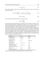
and for systematic reasons a basic distribution is proposed for them as it appears in Fig. 1.

0 50 100 150 200 250 300
Time (sec)
40
60
80
100
120
140
160
180
200
220
Temperature (C)
LISTER LV1
Speed Change: 1440-2125 rpm
Load Change: 32-73%
0 120 240 360 480 600 720
Crank Angle (deg)
0
2
4
6
8

10
12
14
Sur
f
ace Temperature above min. value (deg)
LISTER LV1
Load: 40%
TDC

Fig. 1. Categories of engine unsteady heat conduction phenomena.

Heat Transfer – Engineering Applications

290
As observed any unsteady engine heat transfer phenomenon belongs in either of the
following two basic categories:

Short-term response ones, which are caused by the fluctuations of gas pressure and
temperature during an engine cycle. These are otherwise called cyclic engine heat
transfer phenomena and are developing during a time period in the order of
milliseconds. Phenomena in this category are the result of the physical and chemical
processes developing during the period of an engine cycle. They are finally leading to
the development of temperature and heat flux oscillations in the surface layers of
combustion chamber components. It is noted here that phenomena in this category
should not normally mentioned as “transient” since they are mainly related with
“steady state” engine operation. However their presence during transient engine
operation is as equally important and this is considered in the present work. In addition
the oscillating values of heat conduction variables around the surfaces of combustion
chamber present a “transient” distribution in space since they are gradually faded out

until a distance of a few mm below the surface of each component.

Long-term response ones, resulting from the large time scale non-periodic variations of
engine speed and/or load. As a result, thermal phenomena of this category have a time
“period” in the order of several hundreds of seconds and are presented only during the
transient engine operation.
Each case of long-term response thermal transient can be further separated in two different
phases (Figs 1 and 2). The first of them involves the period from the start of variation until
the instant in which all thermodynamic (combustion gas pressure and temperature, gas
mixture composition etc.) and functional variables (engine torque, speed) reach their final
state of equilibrium. This period lasts a few seconds (usually 3-20) depending on the type of
engine and also on the kind of transient variation under consideration. This first phase of
thermal transient is named as “thermodynamic”.

Thermodynamic phase
time
Start of
transient
A few sec
(depending on governor
and external order)
Several min
Speed, load, cylinder
pressure, temperature in
the final steady state value
Construction
temperatures and heat
fluxes in their final steady
state value
End of

transient
…
Structural Phase

Fig. 2. Phases of long term response thermal transient event.
The upcoming second phase of the transient thermal variation is named as “structural” and
its duration could in some cases overcome the 300 sec until all combustion chamber
components have reached their temperatures corresponding to the final steady state. In the
end of this second phase all variables related with heat conduction in the combustion
chamber (temperatures, heat fluxes) and all heat transfer parameters of the fluids
surrounding the combustion chamber (water, oil etc.) have reached their values
corresponding to the final state of engine transient variation.
Unsteady Heat Conduction Phenomena in Internal
Combustion Engine Chamber and Exhaust Manifold Surfaces

291
Specific examples from the above thermal transient variations are provided in the upcoming
sections.
4. Test engine and experimental measuring installation
4.1 Description of the test engine
A series of experiments concerning unsteady engine heat transfer was conducted by the
author on a single cylinder, Lister LV1, direct injection, diesel engine. The technical data
of the engine are given in Table 1. This is a naturally aspirated, air-cooled, four-stroke
engine, with a bowl-in-piston combustion chamber. All the combustion chamber
components (head, piston, liner etc.) are made from aluminum. The normal speed range is
1000-3000 rpm. The engine is equipped with a PLN fuel injection system. A three-hole
injector nozzle (each hole having a diameter of 0.25 mm) is located in the middle of the
combustion chamber head. The engine is permanently coupled to a Heenan & Froude
hydraulic dynamometer.

Engine type Single cylinder, 4-stroke, air-cooled, DI
Bore/Stroke 85.73 mm/82.55 mm
Connecting rod length 148.59 mm
Compression ratio 18:1
Speed range 1000-3000 rpm
Cylinder dead volume 28.03 cm
3

Maximum power 6.7kW @ 3000 rpm
Maximum torque 25.0 Nm @ 2000 rpm
Inlet valve opening/ closing 15
o
CA before TDC /41
o
CA after BDC
Exhaust valve opening /closing 41
o
CA before BDC /15
o
CA after TDC
Inlet / Exhaust valve diameter 34.5mm / 31.5mm
Fuel pump Bryce-Berger with variable-speed mechanical governor
Injector Bryce- Berger
Injector nozzle opening pressure 190 bar
Static injection timing 28
o
CA before TDC
Specific fuel consumption 259 g/kWh (full load @ 2000 rpm)
Table 1. Engine basic design data of Lister LV1 diesel engine.
The engine experimental test bed was accompanied with the following general purpose

equipment:

Rotary displacement air-flow meter for engine air flow rate measurement

Tank and flow-meter for diesel fuel consumption rate measurement

Mechanical rpm indicator for approximate engine speed readings

Hydraulic brake water pressure manometer, and

Hydraulic brake water temperature thermometer.
4.2 Experimental measuring installation
4.2.1 General
A detailed description of the experimental installation that was used in the present
investigation can be found in previous publications of the author (Mavropoulos et al., 2008,

Heat Transfer – Engineering Applications

292
2009; Mavropoulos, 2011). For that reason, only a brief description will be provided in the
following.
The whole measuring installation was developed by the author in the ICEL Laboratory of
NTUA and was specially designed for addressing internal combustion engine thermal
transient variations (both short- and long-term ones). As a result, its configuration is based
on the separation of the acquired engine signals into two main categories:

Long-term response ones, where the signal presents a non-periodic variation (or
remains essentially steady) over a large number of engine cycles, and

Short-term response ones, where the corresponding signal period is one engine cycle.

To increase the accuracy of measurements, the two signal categories are recorded separately
via two independent data acquisition systems, appropriately configured for each one of
them. For the application in transient engine heat transfer measurements, the two systems
are appropriately synchronized on a common time reference.
4.2.2 Long-term response installation
The long term response set-up comprises ‘OMEGA’ J- and K-type fine thermocouples (14 in
total), installed at various positions in the cylinder head and liner in order to record the
corresponding metal temperatures. Nine of those were installed on various positions and in
different depths inside the metal volume on the cylinder head and they are denoted as
“TH#j” (j=1,…9) in Fig. 3 (a and b). Thermocouples of the same type were also used for
measuring the mean temperatures of the exhaust gas, cooling air inlet, and engine
lubricating oil.
The extensions of all thermocouple wires were connected to an appropriate data acquisition
system for recording. A software code was written in order to accomplish this task.
4.2.3 Short-term response installation
The short-term response installation is in general the most important as far as the periodic
thermal phenomena inside the engine operating cycle are concerned. In general, it presents
the greater difficulty during the set-up and also during the running stage of the
experiments. It comprises the following components:
4.2.3.1 Transducers and heat flux probes
The following transducers were used to record the high-frequency signals during the engine
cycle:

“Tektronix” TDC marker (magnetic pick-up) and electronic ‘rpm’ counter and
indicator.

“Kistler” 6001 miniature piezoelectric transducer for measuring the cylinder pressure,
flush mounted to the cylinder head. Its output signal is connected to a “Kistler” 5007
charge amplifier.


Four heat flux probes installed in the engine cylinder head and the exhaust manifold,
for measuring the heat flux losses at the respective positions. The exact locations of
these probes (HT#1 to 4) and of the piezoelectric transducer (PR#1), are shown in the
layout graph of Fig. 3a and also in the image of Fig. 3b.
The prototype heat flux sensors were designed and manufactured by the author at the
Internal Combustion Engine Laboratory (ICEL) of (NTUA). Additional details and technical
data about them can be found in (Mavropoulos et al., 2008, 2009). They are customized
Unsteady Heat Conduction Phenomena in Internal
Combustion Engine Chamber and Exhaust Manifold Surfaces

293
especially for this application as shown in the images of Fig. 4 where it is presented the
whole instantaneous heat flux measurement system module created and used for the
present investigation. They belong in two different types as described below:

Heat flux sensors (HT#1-3 in Fig. 3a and 3b) installed on the cylinder head, consisting of
a fast response, K-type, flat ribbon, ”eroding” thermocouple, which was custom
designed and manufactured for the needs of the present experimental installation, in
combination with a common K-type, in-depth thermocouple. Each of the fast response
thermocouples was afterwards fixed inside a corresponding compression fitting,
together with the in-depth one that is placed at a distance of 6 mm apart, inside the
metal volume. The final result is shown in Fig. 4.

Inlet
Manifold
Exhaust
Manifold
Injector Hole
HT#1
HT#2

PR#1
HT#4
HT#3
TH#2,
TH#3,
TH#4
TH#1
TH#5,
TH#6
TH#7,
TH#8
TH#9


(a) (b)
Fig. 3. Graphical layout (a), and image (b), of the engine cylinder head instrumented with
the surface heat flux sensors, the piezoelectric pressure transducer and the “long-term”
response thermocouples at selected locations.

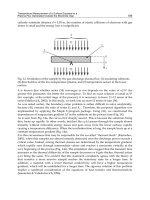
The heat flux sensor installed in the exhaust manifold (HT#4 in Fig. 3a and 3b) has the
same configuration, except that the fast response thermocouple used is a J-type,
“coaxial” one. It is accompanied with a common J-type, in-depth thermocouple, located
inside the compression fitting at a distance of 6 mm behind it. The sensor was flush-
mounted on the exhaust manifold at a distance of 100 mm (when considered in a
straight line) from the exhaust valve.

Heat Transfer – Engineering Applications

294
The heat flux sensors developed in this way displayed a satisfactory level of reliability and

durability, necessary for this application. Also, special care was given to minimize distortion
of thermal field in each position caused by the presence of the sensor. Before being placed to
their final position in the cylinder head and exhaust manifold, all heat flux sensors were
extensively tested and calibrated through a long series of experiments conducted in
different engines, under motoring and firing operating conditions.


Fig. 4. Instantaneous heat flux measurement system module used in the cylinder head and
exhaust manifold wall.
4.2.3.2 Signal pre-amplification and data acquisition system
In order to obtain a clear thermocouple signal when acquiring fast response temperature
and heat flux data, the author had introduced the technique of an initial pre-amplification
stage. This independent pre-amplification stage is applied on the sensor signal before the
latter enters the data acquisition system. The need for such an operation emanates from the
fact that this kind of measurements combines the low voltage level of a thermocouple signal
output with an unusual high frequency. As a result, its direct acquisition using a common
multi-channel data acquisition system creates a great percentage of uncertainty and in some
cases it becomes even impossible. The introduction of pre-amplification stage solves the
previous problems with only a small contribution to signal noise. For recording the fast
response signals during the transient engine operation, the frequency used was in the range
of 4500-6000 ksamples/sec/channel, which resulted in a corresponding signal resolution in
the range of 1-2 deg CA dependent on the instantaneous engine speed.
The prototype preamplifier and signal display device (Fig. 4) was designed and constructed
in the NTUA-ICEL laboratory, using commercially available independent thermocouple
amplifier modules for the J- and K-type thermocouples, respectively. Ten of the above
amplifiers were installed on a common chassis together with necessary selectors and
Unsteady Heat Conduction Phenomena in Internal
Combustion Engine Chamber and Exhaust Manifold Surfaces

295

displays, forming a flexible device that can route the independent heat flux sensor signals
either in the input of an oscilloscope for display and observation, or in the data acquisition
system for recording and storage as it is displayed in Fig. 4. Additional details for the pre-
amplifier can be found in (Mavropoulos et al., 2008, 2009, Mavropoulos, 2011). After the
development of this device by the author, similar devices specialized in fast response heat
flux signal amplification have also become commercially available.
The output signals from the thermocouple pre-amplifier unit, together with the magnetic
TDC pick-up and piezoelectric transducer signals are connected to the input of a high-speed
data acquisition system for recording. Additional details concerning the data acquisition
system are provided in (Mavropoulos, 2011).
5. Presentation and discussion of the simulated and experimental results
5.1 Simulation process and experimental test cases considered
The theoretical investigation of phenomena related to the unsteady heat conduction in
combustion chamber components was based on the application of the simulation model for
engine performance and structural analysis developed by the author. The structural
representation of each component is based on the 3-dimensional FEM analysis code
developed especially for the simulation of thermal phenomena in engine combustion
chamber. For the application of boundary conditions in the various surfaces of each
component, a series of detailed physical models is used. As an example, for the boundary
conditions in the gas side of combustion chamber a thermodynamic simulation model of
engine cycle operation is used in the degree crank angle basis. A brief reference of the
previous models was provided in subsections 2.2 and 2.3. Additional details are available in
previous publications (Rakopoulos & Mavropoulos, 1996, 1999).
Like any other classic FEM code, the thermal analysis program developed consists of the
following three main stages: (a) preprocessing calculations; (b) main thermal analysis; and
(c) postprocessing of the results. An example of these phases of solution is provided in Fig. 5
(a-e) applied in an actual piston and liner geometry of a four stroke diesel engine. For each
of the components a 3-dimensional representation (Fig. 5a) is first created in a relevant CAD
system. In the next step the component is analysed in a series of appropriate 3d finite
elements (Fig. 5b) and the necessary boundary conditions are applied in all surfaces. Then,

during the main analysis the thermal field in each component is solved and this process
could follow several solution cycles until an acceptable convergence in boundary conditions
is achieved. It should be mentioned in this point that due to the complex nature of this
application each combustion chamber component is not independent but it is in contact with
others (for example the piston with its rings and liner etc.). This way the final solution is
achieved when the heat balance equation between all components involved is satisfied.
More details are provided in (Rakopoulos & Mavropoulos, 1998, 1999).
For the postprocessing step one option is a 3d representation of the thermal field variables
(Fig. 5c and 5d). In alternative, a section view (Fig. 5e) is used to describe the thermal field in
the internal areas of the structure in detail. This way the comparison with measured
temperatures in specific points of the component (numbers in parentheses in Fig. 5e) is also
available which is used for the validation of the simulated results.
For the needs of the present investigation several characteristic actual engine transient
events were selected to demonstrate the results of the unsteady heat conduction simulation
model both in the long-term and in the short-term time scale. All of them are performed in

Heat Transfer – Engineering Applications

296
the test engine and the experimental installation described in section 4. For the long-term
scale the following two variations are examined:

A load increment (“variation 1”) from an initial steady state of 2130 rpm engine speed
and 40% of full load to a final one of 2020 rpm speed and 65% of full load.


Fig. 5. Application of the simulation model for engine performance and structural analysis.
A 3d engine piston geometry representation (a), its element mesh (b) and results of thermal
field variables in three (c and d) and two dimensional representations (e).


A speed increment (“variation 2”) from an initial steady state of 1080 rpm engine speed
and 10% of full load to a final one of 2125 rpm speed and 40% of full load.
For the short-term scale the next two transient events are respectively considered:

A change from 20-32% of full load (“variation 3”). During this change, engine speed
remained essentially constant at 1440 rpm. Characteristic feature in this variation was
the slow pace by which the load was imposed (in 10 sec, approximately). For this
transient variation, a total of 357 consecutive engine cycles were acquired in a 30 sec
period via the “short-term response” system signals. For the “long-term response” data
acquisition system, the corresponding figures for this transient variation raised in 3417
consecutive engine cycles during a time period of 285 sec.

Following the previous one, a change from 32-73% of full engine load (“variation 4”)
with a simultaneous increase in engine speed from 1440 to 2125 rpm. In this variation,
the load change was imposed rapidly in an approximate period of 2 sec. This was
accomplished on purpose trying to imitate in the “real engine” the theoretical ramp
variation of engine speed and load. For this transient variation and the “short-term
response” system, 695 engine cycles were acquired in a period of 40 sec. The
Unsteady Heat Conduction Phenomena in Internal
Combustion Engine Chamber and Exhaust Manifold Surfaces

297
corresponding figures for the “long-term response” signals raised in 5035 engine cycles
in a time period of 285 sec.
For all the above transient variations, the initial and final steady state signals were
additionally recorded from both the short- and long-term response installations. Selective
results from the simulation performed and the experiments conducted concerning the
previous four variation cases are presented in the upcoming sections.
5.2 Results concerning long-term heat transfer phenomena in combustion chamber
Before proceeding with the application of the model to transient engine operation cases, it

was first necessary to calibrate the thermostructural submodel under steady state
conditions, especially for the verification of the application of boundary conditions as
described in 2.3. Several typical transient variations (events) of the engine in hand were then
examined which involve increment or reduction of load and/or speed. Results concerning
variation of engine performance variables under each transient event are not presented at
the present work due to space limitations. They are available in existing publications of the
author (Mavropoulos et al., 2009; Rakopoulos et al., 1998; Rakopoulos & Mavropoulos,
2009).
The Finite Element thermostructural model was then applied for the cylinder head of the
Lister-LV1, air-cooled DI diesel engine for which relevant experimental data are available.
For the needs of the present application a mesh of about 50000 tetrahedral elements was
developed, allowing a satisfactory degree of resolution for the most sensitive points of the
construction like the valve bridge area. For the early calculation stages it was found
convenient to utilize a coarser mesh, which helps on the initial application of boundary
conditions furnishing significant computer time economy. The final finer mesh can then be
applied giving the maximum possible accuracy on the final result.
In Fig. 6a the experimental temperature values taken from three of the cylinder head
thermocouples (TH#2-TH#4) during the load increment variation “1”, are compared with
the corresponding calculated ones at the same positions. The calculated curves follow
satisfactorily the experimental ones throughout the progress of the transient event. The
steepest slope between the different curves included in Fig. 6a is observed on the
corresponding ones of thermocouple TH#2 (Fig. 3) placed at the valve bridge area, while the
most moderate one is observed for thermocouple TH#4 placed at the outer surface of the
cylinder head. As expected, the valve bridge is one of the most sensitive areas of the
cylinder head suffering from thermal distortion caused by these sharp temperature
gradients during a transient event (thermal shock). Many cases of damages in the above area
have been reported in the literature, a fact which also confirms the results of the present
calculations.
Similar observations can be made for the cylinder head temperatures in the case of the speed
increment variation “2” presented in Fig. 6b. Again the coincidence between calculated and

experimental temperature profiles is very good. Temperature levels for all positions present
now smaller differences between the initial and final steady state; the steepest temperature
gradient is again observed in the valve bridge area. The initial drop in the temperature value
of thermocouple TH#4 is due to the increase in engine speed for the first few seconds of the
variation which causes a corresponding increase in the air velocity through the fins and so
in the heat transfer coefficient given by eqs (5) to (7) with a simultaneous decrease in air
temperature. From the results presented in Fig. 6 it is concluded that the developed model

Heat Transfer – Engineering Applications

298
manages to simulate satisfactorily the long-term response unsteady heat transfer
phenomena as they are developed in the engine under consideration.

0 50 100 150 200 250 300
Time (sec)
80
90
100
110
120
130
140
150
160
Temperature (deg C)
TH#2 (calculated)
TH#2 (experimental)
TH#3 (calculated)
TH#3 (experimental)

TH#4 (calculated)
TH#4 (experimental)
Load increment: 40% -65%

0 50 100 150 200 250 300
Time (sec)
60
70
80
90
100
110
120
130
140
Temperature (deg C)
TH#2 (calculated)
TH#2 (experimental)
TH#3 (calculated)
TH#3 (experimental)
TH#4 (calculated)
TH#4 (experimental)
Speed increment:
1080 rpm - 2125 rpm

(a) (b)
Fig. 6. Comparison between calculated and experimental temperature profiles vs. time for
three of the cylinder head thermocouples, during the load increment variation “1” (a) and
the speed increment variation “2” (b).
Figs 7 (a and b) present the results of temperature distributions at the whole cylinder head

area in the form of isothermal charts, as they were calculated for the initial and final steady
state of transient variation “1”. Numbers inside squares denote experimental temperature
values recorded from thermocouples. A significant degree of agreement is observed
between the simulated temperature results and the corresponding measured values which
confirms for the validity of the developed model. Similar charts could be drawn for any of
the variations examined and at any specific moment of time during a transient event. They
are presenting in a clear way the local temperature distinctions in the various parts of the
construction, thus they are revealing the mechanism of heat dissipation through the
structure. The observed temperature differences between the inlet and the exhaust valve
side of the cylinder head (exceeding 150
o
C for the full load case) are characteristic for air-
cooled diesel engines, where construction leaves only small metallic common areas between
the inlet and the exhaust side of head. Corresponding results reported in the literature
confirm the above observation (Perez-Blanco, 2004; Wu et al., 2008).
5.3 Results concerning short-term heat transfer phenomena in combustion chamber
During the experiments conducted, the heat flux sensors HT#2 and HT#3 (installed on the
cylinder head) were not able to operate adequately over most of the full spectrum of
measurements taken. The reasons for this failure are described in detail in (Mavropoulos et
al., 2008). Therefore, in this work the short-term results for the cylinder head will be
presented only from sensor HT#1 together with the ones for the exhaust manifold from
sensor HT#4.
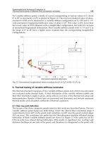
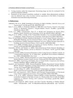
In Figs 8 and 9 are presented the time histories for several of the most important engine
performance and heat transfer variables during the first 2 sec from the beginning of the
transient event for variations “3” and “4”, respectively, which are examined in the present
study. The number of cycles in the first 2 sec of each variation is different as it was expected.
Unsteady Heat Conduction Phenomena in Internal
Combustion Engine Chamber and Exhaust Manifold Surfaces

299

148
126
102
93
137
115
107
113

(a)


50 C
60 C
70 C
80 C
90 C
100 C
110 C
120 C
130 C
140 C
150 C
160 C
170 C
180 C
190 C
200 C
210 C
220 C

230 C
240 C



175
148
115
105
162
138
126
136

(b)
Fig. 7. Cylinder head temperature distributions, in deg. C, at the initial (a) and final (b) state
of the load increment variation “1”. Numbers in “squares” denote experimental temperature
values taken from thermocouples.
The temporal response of cylinder pressure is presented for the two variations in Figs 8a
and 9a, respectively. For variation “3”, an increase of 1-1.5 bar is observed in the peak
pressure during the first 3 cycles of the event. Variation in peak cylinder pressure
becomes marginal after this moment, presents a slight fluctuation and reaches its final
value almost 3 sec after initiation of the variation. For variation “4”, the case is highly
different from the previous one. Pressure changes rapidly and during the first four engine
cycles after the beginning of the transient its peak value is increased linearly from 60 to 80
bar approximately. The 80 bar peak value is maintained afterwards almost constant for a
period of slightly higher than 1 sec, when after approximately the 15th engine cycle it
starts to decline in a slower pace to its final level of 70 bar which corresponds to the final
steady state. The total time period the peak pressure demanded to settle in its final steady
state value for this variation was evaluated to 5 sec. For both variations “3” and “4”, the

time instant after which peak pressure is settled to its final steady state value marks the
end of the first phase of the thermal transient variation that was named as the
“thermodynamic” one. As a result at the end of this phase, the combustion gas has
reached its final steady state. The upcoming second phase of the transient thermal
variation named as the “structural” one is expected to last much longer until all
combustion chamber components have reached their temperatures corresponding to the
final steady state. Additional details about these phases were provided by the author in
(Rakopoulos and Mavropoulos, 1999, 2009). It is in general accepted that the duration of
each period is primarily dependent on the respective duration and also on the magnitude

Heat Transfer – Engineering Applications

300
of speed and/or load change during each specific event. For the present case, the duration
of “thermodynamic” phase is 3 sec for variation “3” and 5 sec for variation “4”,
respectively.
The time histories for the variation of measured wall surface temperature at the position of
sensor HT#1 on cylinder head for the two transient events are presented in Figs 8b and 9b.
In the same Figs they are observed the corresponding wall temperature variations for
depths 1.0-3.0 mm below cylinder head surface inside the metal volume. The last variations
were calculated using the modified one dimensional wall heat conduction model as
described in 2.4. It is observed that wall surface temperature, as being a structural variable,
continues to rise after 2 sec from the beginning of each transient event. However, this
increase in surface temperature refers to its “long-term scale” variation and it is linear in the
case of the moderate load increase of variation “3” (Fig. 8b), or exponential in the case of the
ramp speed and load increase of variation “4” (Fig. 9b). By analysing the whole range of
both experimental measurements it was concluded that the total duration of structural
phase of the transient is estimated at 200 sec for variation “3”, whereas it exceeds 300 sec in
the case of variation “4”. Similar values have been calculated theoretically by the author in
the past using the simulation model for structural thermal field (Rakopoulos and

Mavropoulos, 1999).
Of special importance are the results of measurements presented in Figs 8b and 9b related
to the “short-term scale” that is with reference to the instantaneous cyclic surface
temperatures. In the moderate load increase of variation “3”, the amplitude of
temperature oscillations remains essentially constant during the first 2 sec (and also
during the rest of the event). On the contrary, in the case of the sudden ramp speed and
load increase of variation “4”, a gradual increase is observed in the amplitude of
temperature oscillations during the first four cycles after the beginning of the transient
following the corresponding increase of cylinder pressure in Fig. 9a. However, in the case
of wall surface temperature (x=0.0), its peak values are presented rather unstable and
amplitudes are far beyond the normal ones expected in the case of an aluminum
combustion chamber surface. It is characteristic that the maximum amplitude of
temperature oscillations as presented in Fig. 9b was 31 deg, which is inside the area of
values observed in the case of ceramic materials in insulated engines (Rakopoulos and
Mavropoulos, 1998). These extreme values of temperature oscillations is a clear indication
of abnormal combustion, which occurs in the beginning of variation “4” and it likely lasts
only for about 1.5 sec or the first 21 cycles after the beginning of the transient. After this
period, surface temperature in the combustion chamber returns to its normal fluctuation
and its amplitude is reduced to the value corresponding to the final steady state after
approximately the 50th cycle from the beginning of the transient.
To obtain further insight into the mechanism of heat transfer during a transient operation, it
is useful to examine the temporal development of temperature in the internal layers of
cylinder wall up to a distance of a few mm below the surface. The results for the transient
temperatures during variations “3” and “4” are presented in Figs 8b and 9b for values of
depth x varying from 1.0-3.0 mm below the surface of the cylinder head. In Fig. 8b it is
observed that for transient variation “3” there is no essential difference between the
different engine cycles in each depth during the development of transient event. As
expected the amplitude of temperature oscillations is highly reduced in the internal layers of
Unsteady Heat Conduction Phenomena in Internal
Combustion Engine Chamber and Exhaust Manifold Surfaces

301
cylinder head volume and for x=3.0 mm below the combustion chamber surface practically
there exists no temperature oscillation. On the other hand during transient variation “4” in
Fig. 9b, the abnormal combustion indicated previously causes the development of a heat
wave penetrating quickly in the internal layers of cylinder head. It is remarkable that during
the first 20 cycles from the beginning of the event, temperature swings of 0.7 deg can be
sensed even in a depth of x=3.0 mm below the surface of combustion chamber. The instant
velocity of this penetration during the transient event “4” can also be estimated from the
results presented in Fig. 9b. From the analysis of the results it was observed that the peak
temperature in the depth of x=3.0 mm below the surface appears at an angle of 720 deg. As a
consequence, during an approximate “time period” of 360 deg the thermal wave penetrates
3.0 mm inside the metallic volume of cylinder head. After the 20th cycle the temperature
oscillations start to reduce and after a few more engine cycles are vanished in the depth of
3.0 mm below surface.
Following the above analysis for surface temperature, heat flux time histories for the point
of measurement (HT#1) in the cylinder head and the two variations examined, are
presented in Figs 8c and 9c. Heat flux histories are highly influenced by gas pressure and
surface temperature variations, and their patterns are in general similar with them. In the
case of variation “3”, a mild increase in peak cylinder heat flux is observed during the first
four cycles of the event and this is due to the similar increase observed in cylinder
pressure during the same period. There is a marginal increase in peak values afterwards
due to surface temperature increase and the final steady state peak value is reached after
the 50th cycle, approximately. In variation “4”, the heat flux is rather unstable following
the pattern of surface temperatures. Due to the combustion instabilities described
previously, measured peak heat flux values raised to almost three times higher than the
ones observed during the normal engine operation, the highest of them reaching the value
9000 kW/m
2
corresponding to the same cycles in which the extreme surface temperature

values have occurred. Peak heat flux is reduced afterwards at a slower pace to its final
steady-state value, which is reached after the 200th cycle from the beginning of the event.
A similar form of instantaneous heat flux variation during the first cycles of the warm-up
period for a spark ignited engine was presented by the authors of (Wang & Stone, 2008).
5.4 Unsteady heat conduction phenomena in the engine gas exchange system
Phenomena related with the unsteady heat transfer in the inlet and exhaust engine
manifolds are of special interest. In particular during the last years these phenomena have
drawn special attention due to their importance in issues related with pollutant emissions
during transient engine operation and especially the combustion instability which occurs in
the case of an engine cold-starting event.
The variation of surface temperature and heat flux in the engine exhaust manifold follows in
general the same trends as in the cylinder head. In this case, since the point of temperature
and heat flux measurement was placed 100 mm downstream the exhaust valve (Figs 3 and
4), the corresponding phenomena are significantly faded out (Figs 10 and 11).
Increase of the amplitude of temperature oscillations is again obvious for variation “4” (Fig.
11a). However, there are no extreme amplitudes present in this case, as they have been
absorbed due to the transfer of heat to the cylinder and manifold walls along the 100 mm
distance from the exhaust valve to the point of measurement.

Heat Transfer – Engineering Applications

302
0.0 0.2 0.4 0.6 0.8 1.0 1.2 1.4 1.6 1.8 2.0
Time (sec)
0
500
1000
1500
2000
2500

3000
Heat Flux (kW/m
2
)

(c)

0.0 0.2 0.4 0.6 0.8 1.0 1.2 1.4 1.6 1.8 2.0
Time (sec)
200
210
220
230
240
250
260
270
Wall Tempe
r
atu
r
e (C)
Cylinder Head
x=0.0 mm
x=1.0 mm
x=2.0 mm
x=3.0 mm

(b)

0.0 0.2 0.4 0.6 0.8 1.0 1.2 1.4 1.6 1.8 2.0
Time (sec)
01234567891011121314151617181920212223
Cycle No (-)
0
10
20
30
40
50
60
70
Cylinder Pressure (bar)
LISTER LV1
Speed Change: ct (1440 rpm)
Load Change: 20-32%

(a)

Fig. 8. Time histories of cylinder pressure (a), wall temperature for cylinder head on surface
x=0.0 and three different depths inside the metal volume (b) and heat flux variation for
cylinder head (c), for the first 2 sec of transient variation “3”.
Unsteady Heat Conduction Phenomena in Internal
Combustion Engine Chamber and Exhaust Manifold Surfaces

303
0.0 0.2 0.4 0.6 0.8 1.0 1.2 1.4 1.6 1.8 2.0
Time (sec)
0
1000

2000
3000
4000
5000
6000
7000
8000
9000
10000
Heat Flux (kW/m
2
)

(c)

0.0 0.2 0.4 0.6 0.8 1.0 1.2 1.4 1.6 1.8 2.0
Time (sec)
210
220
230
240
250
260
270
280
290
300
Wall Tempe
r
atu

r
e (C)
Cylinder Head
x=0.0 mm
x=1.0 mm
x=2.0 mm
x=3.0 mm

(b)

0.0 0.2 0.4 0.6 0.8 1.0 1.2 1.4 1.6 1.8 2.0
Time (sec)
0 1 2 3 4 5 6 7 8 9 10 11 12 13 14 15 16 17 18 19 20 21 22 23 24 25 26 27 28
Cycle No (-)
0
10
20
30
40
50
60
70
80
90
Cylinder Pressure (bar)
LISTER LV1
Speed Change: 1440-2125 rpm
Load Change: 32-73%

(a)

Fig. 9. Time histories of cylinder pressure (a), wall temperature for cylinder head on surface
x=0.0 and three different depths inside the metal volume (b) and heat flux variation for
cylinder head (c), for the first 2 sec of transient variation “4”.

Heat Transfer – Engineering Applications

304
0.0 0.2 0.4 0.6 0.8 1.0 1.2 1.4 1.6 1.8 2.0
Time (sec)
0
50
100
150
200
250
300
Heat Flux (kW/m
2
)

(b)

0.0 0.2 0.4 0.6 0.8 1.0 1.2 1.4 1.6 1.8 2.0
Time (sec)
0 1 2 3 4 5 6 7 8 9 1011121314151617181920212223
Cycle No (-)
106
107
108

109
110
111
112
Wall Tempe
r
atu
r
e (C)
Exhaust Manifold
LISTER LV1
Speed Change: ct (1440 rpm)
Load Change: 20-32%

(a)

Fig. 10. Time histories of exhaust manifold wall surface temperature (a) and heat flux (b) at
the position of sensor HT#4 for the first 2 sec of transient variation “3”.
The corresponding results for heat flux time histories in the point of measurement on the
exhaust manifold are presented in Figs 10b and 11b. In the case of variation “3”, the
moderate load increase is reflected as a marginal increase in exhaust manifold heat flux (a
difference cannot be observed in time history of Fig. 10b). In the case of ramp variation “4”
on the other hand, it is observed in Fig 11b a sudden increase in the amplitude of exhaust
manifold heat flux, which starts 4 cycles after the beginning of the transient. In this case,
there is no gradual increase of heat flux amplitude during the first four cycles, as it was the
case for cylinder pressure and also cylinder head surface temperature and heat flux. Like the
case of exhaust manifold surface temperature, this result is due to the heat transfer to
combustion chamber and exhaust manifold walls until the point of measurement. It is
observed that during the first 20 cycles of variation “4” the heat losses to exhaust manifold
walls are increased beyond their normal level, due to increased engine speed and

consequently gas velocity inside the exhaust manifold. The latter is the primary factor
influencing heat losses in the exhaust manifold, as shown in (Mavropoulos et al., 2008). The
Unsteady Heat Conduction Phenomena in Internal
Combustion Engine Chamber and Exhaust Manifold Surfaces

305
increased level of heat losses during the gas exchange period of each cycle for the first 20
cycles is the reason for the appearance of negative heat fluxes in the results of Fig. 11b. Such
a case is quite remarkable and could not appear in the position of measurement during
steady state operation. Heat flux becomes negative (that is heat is transferred from manifold
wall to the gas) for a short period of engine cycle after TDC. This coincides with the period
during which combustion gas temperature at the distance of 100 mm downstream the
exhaust valve inside the manifold reaches its minimum value. The combination of
instantaneous exhaust gas temperature with gas velocity at the point of measurement is the
reason for the final result concerning the time history of heat flux in the exhaust manifold.

0.0 0.2 0.4 0.6 0.8 1.0 1.2 1.4 1.6 1.8 2.0
Time (sec)
-400
-200
0
200
400
600
800
Heat Flux (kW/m
2
)

(b)

0.0 0.2 0.4 0.6 0.8 1.0 1.2 1.4 1.6 1.8 2.0
Time (sec)
012345678910111213141516171819202122232425262728
Cycle No (-)
115
120
125
130
135
140
145
Wall Tempe
r
atu
r
e (C)
Exhaust Manifold
LISTER LV1
Speed Change: 1440-2125 rpm
Load Change: 32-73%

(a)
Fig. 11. Time histories of exhaust manifold wall surface temperature (a) and heat flux (b) at
the position of sensor HT#4 for the first 2 sec of transient variation “4”.
6. Conclusion
A theoretical simulation model accompanied with a comprehensive experimental procedure
was developed for the analysis of unsteady heat transfer phenomena which occur in the
combustion chamber and exhaust manifold surfaces of a DI diesel engine. The results of the

Heat Transfer – Engineering Applications

306
study clearly reveal the influence of transient engine heat transfer phenomena both in the
engine structural integrity as well as in its performance aspects. The main findings from the
analysis results of the present investigation can be summarized as follows:

Thermal phenomena related to unsteady heat transfer in internal combustion engines
can be categorized as long- or short-term response ones in relation to the time period of
their development. Each long-term response variation is further separated to a
“thermodynamic” and a “structural” phase.

Calculated temperature profiles from the Finite Element sub-model matched
satisfactorily the corresponding experimental temperature profiles recorded by the
thermocouples, revealing that the area between the two valves (valve bridge) is the
most sensitive one towards the generation of sharp temperature gradients during each
transient (thermal shock). The effect of air velocity in the cooling procedure of external
surfaces is clearly revealed and analysed.

A strong influence exists between the long-term non-periodic heat transfer variation
resulting from engine transient operation and the instantaneous cyclic short-term
responses of surface temperatures and heat fluxes. The results of this interaction
influence primarily the combustion chamber and secondary the exhaust manifold
surfaces.

In the first cycles (“thermodynamic” phase) of a ramp engine transient, abnormal
combustion occurred. The result is that the amplitude of surface temperature swings
and the peak heat flux value for cylinder head surfaces were increased at extreme
values, reaching almost 3 times the level of the corresponding ones that occur during
steady state operation.


The respective phenomena inside the exhaust manifold at a distance of 100 mm
downstream the exhaust valve have a minor impact on the local surfaces. Temperature
gradients are reduced in low levels due to heat losses. The gas velocity inside the
exhaust manifold is the main factor influencing heat transfer and wall heat losses.
7. References
Annand, W.J.D. (1963). Heat transfer in the cylinders of reciprocating internal combustion
engines.
Proceedings of the Institution of Mechanical Engineers, Vol.177, pp. 973-990
Assanis, D. N. & Heywood, J. B. (1986). Development and use of a computer simulation of
the turbocompounded diesel engine performance and component heat transfer
studies.
Transactions of SAE, Journal of Engines, Vol.95, SAE paper 860329
Demuynck, J., Raes, N., Zuliani, M., De Paepe, M., Sierens, R. & Verhelst, S. (2009). Local
heat flux measurements in a hydrogen and methane spark ignition engine with a
thermopile sensor.
Int. J Hydrogen Energy, Vol.34, No.24, pp. 9857-9868
Heywood, J.B. (1998).
Internal Combustion Engine Fundamentals, McGraw-Hill, New York
Keribar, R. & Morel, T. (1987). Thermal shock calculations in I.C. engines, SAE paper
870162
Lin, C.S. & Foster, D.E. (1989). An analysis of ignition delay, heat transfer and combustion
during dynamic load changes in a diesel engine, SAE paper 892054
Mavropoulos, G.C., Rakopoulos, C.D. & Hountalas, D.T. (2008). Experimental assessment of
instantaneous heat transfer in the combustion chamber and exhaust manifold walls
Unsteady Heat Conduction Phenomena in Internal
Combustion Engine Chamber and Exhaust Manifold Surfaces

307
of air-cooled direct injection diesel engine. SAE International Journal of Engines,
Vol.1, No.1, (April 2009), pp. 888-912, SAE paper 2008-01-1326

Mavropoulos, G.C., Rakopoulos, C.D. & Hountalas, D.T. (2009). Experimental investigation
of instantaneous cyclic heat transfer in the combustion chamber and exhaust
manifold of a DI diesel engine under transient operating conditions, SAE paper
2009-01-1122
Mavropoulos, G.C. (2011). Experimental study of the interactions between long and short-
term unsteady heat transfer responses on the in-cylinder and exhaust manifold
diesel engine surfaces.
Applied Energy, Vol.88, No.3, (March 2011), pp. 867-881
Perez-Blanco, H. (2004). Experimental characterization of mass, work and heat flows in an
air cooled, single cylinder engine.
Energy Conv. Mgmt, Vol.45, pp. 157-169
Rakopoulos, C.D. & Mavropoulos, G.C. (1996). Study of the steady and transient
temperature field and heat flow in the combustion chamber components of a
medium speed diesel engine using finite element analyses.
International Journal of
Energy Research
, Vol.20, pp. 437-464
Rakopoulos, C.D. & Mavropoulos, G.C. (1998). Components heat transfer studies in a low
heat rejection DI diesel engine using a hybrid thermostructural finite element
model.
Applied Thermal Engineering, Vol.18, pp. 301-316
Rakopoulos, C.D., Mavropoulos, G.C. & Hountalas, D.T. (1998). Modeling the structural
thermal response of an air-cooled diesel engine under transient operation
including a detailed thermodynamic description of boundary conditions, SAE
paper 981024
Rakopoulos, C.D. & Hountalas, D.T. (1998). Development and validation of a 3-D multi-
zone combustion model for the prediction of DI diesel engines performance and
pollutants emissions.
Transactions of SAE, Journal of Engines, Vol.107, pp. 1413-1429,
SAE paper 981021

Rakopoulos, C.D. & Mavropoulos, G.C. (1999). Modelling the transient heat transfer in the
ceramic combustion chamber walls of a low heat rejection diesel engine.
International Journal of Vehicle Design, Vol.22, No.3/4, pp. 195-215
Rakopoulos, C.D. & Mavropoulos, G.C. (2000). Experimental instantaneous heat fluxes in
the cylinder head and exhaust manifold of an air-cooled diesel engine.
Energy
Conversion and Management
, Vol.41, pp. 1265-1281
Rakopoulos, C.D., Rakopoulos, D.C., Giakoumis, E.G. & Kyritsis, D.C. (2004). Validation
and sensitivity analysis of a two-zone diesel engine model for combustion and
emissions prediction.
Energy Conversion and Management, Vol.45, pp. 1471-1495
Rakopoulos, C.D. & Mavropoulos, G.C. (2008). Experimental evaluation of local
instantaneous heat transfer characteristics in the combustion chamber of air-cooled
direct injection diesel engine.
Energy, Vol.33, pp. 1084–1099
Rakopoulos, C.D. & Mavropoulos, G.C. (2009). Effects of transient diesel engine operation
on its cyclic heat transfer: an experimental assessment.
Proc. IMechE, Part D: Journal
of Automobile Engineering,
Vol.223, No.11, (November 2009), pp. 1373-1394
Sammut, G. & Alkidas, A.C. (2007). Relative contributions of intake and exhaust tuning on
SI engine breathing-A computational study, SAE paper 2007-01-0492

Heat Transfer – Engineering Applications

308
Wang, X. and Stone, C.R. (2008). A study of combustion, instantaneous heat transfer, and
emissions in a spark ignition engine during warm-up.
Proc. IMechE, Vol.222, pp.

607-618
Wu, Y., Chen, B., Hsieh, F. & Ke, C. (2008). Heat transfer model for scooter engines, SAE
paper 2008-01-0387
13
Ultrahigh Strength Steel: Development
of Mechanical Properties
Through Controlled Cooling
S. K. Maity
1
and R. Kawalla
2

1
National Metallurgical Laboratory,
2
TU Bergademie,
1
India
2
Germany
1. Introduction
Structural steels with very high strength are referred as ultrahigh strength steels. The
designation of ultrahigh strength is arbitrary, because there is no universally accepted
strength level for this class of steels. As structural steels with greater and greater strength
were developed, the strength range has been gradually modified. Commercial structural
steel possessing a minimum yield strength of 1380 MPa (200 ksi) are accepted as ultrahigh
strength steel (Philip, 1990). It has many applications such as in pipelines, cars, pressure
vessels, ships, offshore platforms, aircraft undercarriages, defence sector and rocket motor
casings. The class ultrahigh strength structural steels are quite broad and include several
distinctly different families of steels such as (a) medium carbon low alloy steels, (b) medium

alloy air hardening steel, (c) high alloy hardenable steels, and (d) 18Ni maraging steel. In the
recent past, developmental efforts have been aimed mostly at increasing the ductility and
toughness by improving the melting and the processing techniques. Steels with fewer and
smaller non-metallic inclusions are produced by use of selected advanced processing
techniques such as vacuum deoxidation, vacuum degassing, vacuum induction melting,
vacuum arc remelting (VAR) and electroslag remelting (ESR). These techniques yield (a) less
variation of properties from heat to heat, (b) greater ductility and toughness especially in the
transverse direction, and (c) greater reliability in service (Philip, 1978).

The strength can be
further increased by thermomechanical treatment with controlled cooling.
1.1 Medium carbon low alloy steel
The medium carbon low alloy family of ultra high strength steel includes AISI/SAE 4130,
the high strength 4140, and the deeper hardening and high strength 4340. In AMS 6434,
vanadium has been added as a grain refiner to improve the toughness and carbon is
reduced slightly to improve weldability. D-6a contains vanadium as grain refiner, slightly
higher carbon, chromium, molybdenum and slightly lower nickel than 4340. Other less
widely used steels that may be included in this family are 6150 and 8640. Medium-carbon
low alloy ultrahigh strength steels are hot forgeable, usually at 1060 to 1230C. Prior to

Heat Transfer – Engineering Applications

310
machining, the usual practice is to normalise at 870 to 925C and temper at 650 to 675C.
These treatments yield moderately hard structures consisting of medium to fine pearlite. It
is observed that maximum tensile strength and yield strength result when these steels are
tempered at 200C. With higher tempering temperature, the mechanical properties drop
sharply. The mechanical properties obtained in oil-quenched and tempered conditions are
shown in Table 1.

Designation
Tempering
temperature
(C)
Tensile
strength
(MPa)
Yield
strength
(MPa)
Elongation
(%)
Hardness
(HB)
Izod
impact
(J)
Fracture
toughness
(MPam)
4130
205
425
1550
1230
1340
1030
11
16.5

450
360
-
-
70
4140
205
425
1965
1450
1740
1340
11
15
578
429
15
28
49
4340
205
425
1980
1500
1860
1365
11
14
520
440

20
16
46-AM
60- VAR
300M
205
425
2140
1790
1650
1480
7.0
8.5
550
450
21.7
13.6
-
D – 6a
205
425
2000
1630
1620
1570
8.9
9.6
-
-
15

16
99
Table 1. Mechanical properties of medium carbon alloy steel.
1.2 Medium alloy air hardening steel
The steels H11, Modified (H11 Mod) and H13 are included in this category. These steels are
often processed through remelting techniques like VAR or ESR. VAR and ESR produced
H13 have better cleanness and chemical homogeneity than air melted H13. This results in
superior ductility, impact strength and fatigue resistance, especially in the transverse
direction, and in large section size. Besides being extensively used in dies, these steels are
also widely used for structural purposes. They have excellent fracture toughness coupled
with other mechanical properties. H11 Mod and H13 can be hardened in large sections by
air-cooling. The chemical compositions and the mechanical properties of these steels are
given in Table 2.


Designation C (%) Mn (%) Si (%) Cr (%) Mo (%) V(%)
H11 Mod 0.37 – 0.43 0.20 – 0.40 0.80 – 1.00 4.74 – 5.25 1.20 – 1.40 0.40 – 0.60
H13 0.32 – 0.45 0.20 – 0.50 0.80 – 1.20 4.75 – 5.50 1.10 – 1.75 0.80 – 1.20

Designation
Tempering
temperature
(C)
Tensile
strength
(MPa)
Yield
strength
(MPa)
Elongation

(%)
Hardness
(HRc)
Izod impact
(J)
H11 Mod 565 1850 1565 11 52 26.4
H13 575 1730 1470 13.5 48 27
Table 2. Chemical compositions and mechanical properties of medium alloy air hardening
ultra high strength steel.
Ultrahigh Strength Steel: Development of
Mechanical Properties Through Controlled Cooling

311
1.3 High alloy hardenable steel
These steels were introduced by Republic Steel Corporation in the 1960’s and have four
weldable steel grades with high fracture toughness and yield strength in heat treated
condition. These nominally contain 9% Ni and 4% Co and differ only in carbon content. The
four steels designated as HP9-4-20, HP9-4-25, HP9-4-30 and HP9-4-45 nominally have 0.20,
0.25, 0.30 and 0.45%C respectively. Among these steels, HP9-4-20 and HP9-4-30 are
produced in significant quantities and their chemical composition and mechanical
properties are given in Table 3 (Philip, 1978). As the carbon content of these steels increases,
attainable strength increases with corresponding decrease in both toughness and
weldability. The high nickel content of 9% provides deep hardenability, toughness and some
solid solution strengthening. If the steel contains only higher amount of nickel but no cobalt,
there would be a strong tendency for retention of large amounts of austenite on quenching.
This retained austenite would not decompose even by refrigeration and tempering. Cobalt
increases the Ms temperature and counteracts austenite retention. Chromium and
molybdenum content are kept low for improvement of toughness. Silicon and other
elements are kept as low as practicable.

Designation
C
(%)
Mn
(%)
Si
(%)
Cr
(%)
Ni
(%)
Mo
(%)
V
(%)
Others
(%)
HP 9-4-20
0.16–
0.23
0.20–
0.40
0.20
max
0.65–0.85 8.50–9.50 0.90–1.10 0.06–0.12
4.25– 4.75
Co
HP 9-4-30
0.29–
0.34

0.10–
0.35
0.20
max
0.90–1.10 7.0 – 8.0 0.90–1.10 0.06–0.12
4.25– 4.75
Co

Designation
Tensile
strength
(MPa)
Yield
strength
(MPa)
Elongation
(%)
Hardness
(HRc)
Izod impact
(J)
HP 9-4-20 1380 - - - -
HP 9-4-30 1650 1350 14 49 - 53 39
Table 3. Chemical compositions and typical mechanical properties of high alloy hardenable
ultra high strength steel.
1.4 18 Ni maraging steel
Steels belonging to this class of high strength steels differ from other conventional steels.
These are not hardened by metallurgical reactions that involve carbon, but by the
precipitation of intermetallic compounds at temperatures of about 480C. The typical yield
strengths are in the range 1030 MPa to 2420 MPa. They have very high nickel, cobalt and

molybdenum and very low carbon content. The microstructure consists of highly alloyed
low carbon martensites. On slow cooling from the austenite region, martensite is produced
even in heavy sections, so there is no lack of hardenabilty. Cobalt increases the Ms
transformation temperature so that complete martensite transformation can be achieved.
The martensite is mainly body centred cubic (bcc), and has lath morphology. Maraging steel
normally contains little or no austenite after heat treatment. The presence of titanium leads
to precipitation of Ni
3
Ti. It gives additional hardening. However, high titanium content
favours formation of TiC at the austenite grain boundaries, which can severely embrittle the

Heat Transfer – Engineering Applications

312
age-hardened steel (Philip, 1978). The nominal chemical compositions of the commercial
maraging steels are shown in Table 4. Typical tensile properties are shown in Table 5.
One of the distinguishing features of the maraging steels is their superior toughness
compared to conventional steels. Maraging steels are normally solution annealed
(austenitised) and cooled to room temperature before aging. Cooling rate after annealing
has no effect on microstructure. Aging is normally done at 480C for 3 to 6 hours. These
steels can be hot worked by conventional steel mill techniques. Working above 1260C
should however be avoided (Floreen, 1978). Maraging steels have found varieties of
applications including missile casing, aircraft forgings, special springs, transmission shafts,
couplings, hydraulic hoses, bolts and punches and dies.

Grade
C
(%)
Ni
(%)

Mo
(%)
Co
(%)
Ti
(%)
Al
(%)
Other
(%)
18Ni (200) 0.03 max 18 3.3 8.5 0.2 0.1 -
18Ni (250) 0.03 max 18 5.0 8.5 0.4 0.1 -
18Ni (300) 0.03 max 18 5.0 9.0 0.7 0.1 -
18Ni (350) 0.03 max 18 4.2 12.5 1.6 0.1 -
18Ni (cast) 0.03 max 17 4.6 10.0 0.3 0.1 -
18Ni (180) 0.03 max 12 3 - 0.2 0.3 5.0% Cr
Table 4. The nominal chemical compositions of maraging steel.

Grade Heat treatment
Tensile strength
(MPa)
Yield strength
(MPa)
Elongation
(%)
18Ni (200) A 1500 1400 10
18Ni (250) A 1800 1700 8
18Ni (300) A 2050 2000 7
18Ni (350) B 2450 2400 6
18Ni (cast) C 1750 1650 8

A: solution treat 1h at 820C, aging 3h at 480C; B: solution treat 1h at 820C, aging 12h at 480C;
C: anneal 1h at 1150C, aging 1h at 595C, solution treat 1h at 820C, aging 3h at 480C.
Table 5. Mechanical properties of the heat treated maraging steel.

1.5 Issues and objective
In addition to high strength-to-weight ratio, ultra high strength steels should possess good
ductility, toughness, fatigue resistance and weldability. Some of the currently employed
steels, like maraging steels, are highly alloyed and are expensive. Search for less expensive
steels with better properties, is therefore a continuing process. High strength in these alloys
is obtained by exploiting all the strengthening mechanisms, by careful control of alloying
and subsequent processing. Often when strength is raised by alloying and
thermomechanical treatment, ductility and toughness suffer. Additionally one can have
serious problems with fatigue properties. Many defects are introduced, and inferior
properties are obtained during the solidification process. It is, therefore, advantageous to
exercise great control during this process. Secondary refining processes like vacuum arc
remelting (VAR) and electroslag refining (ESR) are often employed to obtain superior
Ultrahigh Strength Steel: Development of
Mechanical Properties Through Controlled Cooling

313
properties in these materials for critical applications. Electroslag refining is known to give
low inclusion content, low macro-and micro-segregation, and low microporosity due to
near-directional solidification from a small pool with application of controlled cooling.
Many alloys for critical application now use this process to ensure reliability and good
properties.
The material developed earlier at Indian Institute of Technology (IIT) Bombay and Vikram
Saravai Space Center (VSSC), Trivandrum, India with a yield strength of 1450 MPa, is
qualified as aerospace application (Suresh et al., 2003; Chatterjee et al., 1990). This was a
medium-carbon low alloy steel used mostly in tempered condition. The chemical
composition of the alloy is: 0.3% C, 1.0% Mn, 1.0% Mo, 1.5% Cr, 0.3% V and named as 0.3C-

CrMoV (ESR) steel (Suresh et al, 2003). The microstructure of heat treated alloy primarily
consists of tempered lath martensite. The primary objective of the present work is to
develop an alloy with yield strength in excess of 1700 MPa with adequate ductility and
impact toughness. It has been achieved through:
a. ESR processing of the alloys
b. Thermomechanical treatment with controlled cooling
1.6 Plan of investigation
UHSS is mostly developed by interplay of all strengthening mechanisms. Grain refinement
is achieved either by fine precipitates which pin the austenite grain boundaries by micro
alloys (Tanaka, 1981; Umemoto et al., 1987). Precipitation of carbides and carbonitrides both
at high temperatures or during cooling and tempering helps to improve the mechanical
properties for specific needs (Bleck et al., 1988).

Ductility and toughness suffer in most
methods of strengthening when one tries to increase strength. The approach in the present
work, therefore, is to adjust the chemistry and optimise the production process to obtain
clean steel with finer microstructures by special melting process. Therefore, it is
advantageous to process these materials through a secondary refining process like
electroslag refining (ESR), which ensures the cleanliness and chemical homogeneity (Shash,
1988; Choudhary & Szekely, 1981). Further improvement of mechanical properties is to be
obtained by a control thermomechanical treatment (TMT). Melting and casting of alloys and
subsequent processing like TMT are the two main aspects in this study.
In the first part of the study, the alloys were prepared with variation of chemical
composition starting with a basic composition of 0.3%C, 4.2%Cr, 1%Mn, 1%Mo and 0.35%V.
In the previous study, the effects addition of titanium and niobium, and increase of
chromium and vanadium

contents on the mechanical and microstructural properties were
investigated (Maity et al., 2008a, 2008b).

Most of these alloys in as cast tempered condition
displayed minimum yield strengths of 1450 MPa with elongation of about 9-12% and impact
toughness in many cases was in excess of 300 kJ.m
-2
. For further improvement of mechanical
properties especially to increase the toughness values, the basic steel is alloyed with 1-3% of
nickel in this study. Nickel is generally added in many low alloy steels to improve low
temperature toughness and hardenability (Maity et al., 2009).

It also strengthens the steel by
solid solution hardening, and is particularly effective when it is used in combination with
chromium and molybdenum (Umemoto et al., 1987).

Nickel is known to increase the
resistance to cleavage fracture in steel and decreases ductile-to-brittle transition
temperature. The medium-carbon low-alloy martensitic steel attains the best combination of
properties in tempered condition owing to the formation of transition carbides