Hydrodynamics Natural Water Bodies Part 5 pot
Bạn đang xem bản rút gọn của tài liệu. Xem và tải ngay bản đầy đủ của tài liệu tại đây (409.51 KB, 25 trang )
Challenges and Solutions for Hydrodynamic and Water Quality in Rivers in the Amazon Basin
87
Richey, J. E., Meade, R. H., Salati, E., Devol, A. H., Nordin, C. F., & Santos, U. Water
discharge and suspended sediment concentrations in the Amazon River: 1982-1984.
Water Resour. Res. 22 , 756-764, 1986.
Rosman, P. C. Referência Técnica do Sistema Base de Hidrodinâmica Ambiental. Versão
11/12/2007. 211 p. COPPE/UFRJ. Rio de Janeiro. 2007.
Sekiguchi, H., Watanabe, M., Nakahara, T., Xu, B. H., & Uchiyama, H. Succession of
bacterial community structure along the Changjiang River determined by
denaturing gradient gel electrophoresis and clone library analysis. Appl. Environ.
Microbiol, 181-188, 2002.
Shen, C; Niu, J. Anderson, E. J; & Phanikumar, M. S. Estimating longitudinal dispersion in
rivers using Acoustic Doppler Current Profilers. Advances in Water Resources. 33.
615-623, 2010.
Silva, M. S.; Kosuth, P. Comportamento das vazões do rio Matapi em 27.10.2000. Congresso
da Associação Brasileira de Estudos do Quaternário, 8. Imbé-RS. Resumos,
ABEQUA, p. 594-596. 2001.
Smith Jr, W. O. & DeMaster, D. J. Phytoplankton biomass and productivity in the Amazon
River plume: correlation with seasonal river discharge. Continental Shelf Research 6 ,
227-244, 1995.
Souza, E. B. & Cunha, A. C. Climatologia de precipitação no Amapá e mecanismos
climáticos de grande escala. In: A. C. Cunha, E. B. Souza, e H. F. Cunha, Tempo,
clima e recursos hídricos: Resultados do projeto REMETAP no Estado do Amapá (pp. 177-
195). Macapá-AP: IEPA, 2010.
Souza, E. B. Precipitação sazonal sobre a Amazônia Oriental no período chuvoso:
observações e simulações regionais com o RegCM3. Revista Brasileira de Meteorologia
, v. 24, n. 2, 111 – 124, 2009.
Stevaux, J. C; Franco, A. A; Etchebehere, M. L. C & Fujita, R. H. Flow structure and
dynamics in large tropical river confluence: example of the Ivaí and Paraná rivers,
southern Brazil. Geociências. São Paulo. V.28, n.1, p. 5-13, 2009.
Stone, M. C. & Hotchkiss, R. H. Evaluating velocity measurement techniques in shallow
streams. Journal of Hydraulic Research. Vol. 45, No. 6, pp. 752–762, 2007.
Subramaniam, A., Yager, P. L., Carpenter, E. J., Mahaffey, C., Biörkman, K. & Cooley, S.
Amazon River enhances diazotrophy and carbon sequestration in the tropical
North Atlantic Ocean. Science. 105(30) , pp. 10460-10465, 2008.
Unger, D., Ittekkot, V., Schafer, P. & Tiemann, J. Biogeochemistry of particulate organic
matter from the Bay of Bengal as discernible from hydrolysable neutral
carbohydrates and amino acids. Marine Chemistry 96 , 155, 2005.
Van Maren, D. S. & Hoekstra, P. Seasonal variation of hydrodynamics and sediment
dynamics in a shallow subtropical estuary: the Ba Lat River, Vietnam. Estuarine,
Coastal and Shelf Science. 60, 529e540, 2004.
Versteeg, H. K. & Malalasekera, W. An introduction to computational fluid dynamics: the
finite volume method. Prentice Hall. 257p. 1995.
Voss, M., Bombar, D., Loick, N. & Dippner, J. Riverine influence on nitrogen fixation in the
upwelling region off Vietnam, South China Sea. Geophysical Research Letters, 33 ,
L07604, doi:10.1029/2005GL025569, 2006.
Hydrodynamics – Natural Water Bodies
88
Wasman, P. Retention versus export food chains: processes controlling sinking loss from
marine pelagic systems. Hydrobiologia 363 , 29-57, 1988.
5
Hydrodynamic Pressure Evaluation of
Reservoir Subjected to Ground
Excitation Based on SBFEM
Shangming Li
Institute of Structural Mechanics, China Academy of Engineering Physics
Mianyang City, Sichuan Province
China
1. Introduction
Dynamic responses of dam-reservoir systems subjected to ground motions are often a major
concern in the design. To ensure that dams are adequately designed for, the hydrodynamic
pressure distribution along the dam-reservoir interface must be determined for assessment
of safety.
Due to the fact that analytical methods are not readily available for dam-reservoir systems
with arbitrary geometry shape, numerical methods are often used to analyze responses of
dam-reservoir systems. In numerical methods, dams are often discretized into solid finite
elements through Finite Element Method (FEM), while the reservoir is either directly
modeled by Boundary Element Method (BEM) or is divided into two parts: a near field with
arbitrary geometry shape and a far field with a uniform cross section. The near field is
discretized into acoustic fluid finite elements by using FEM or boundary elements by BEM,
while the far field is modeled by BEM or a Transmitting Boundary Condition (TBC). Based
on these numerical methods, several coupling procedures were developed.
A FEM-BEM coupling procedure was used to implement the linear and non-linear analysis
of dam-reservoir interaction problems (Tsai & Lee, 1987; Czygan & Von Estorff, 2002),
respectively, in which the dam was modeled by FEM, while the reservoir was modeled by
BEM. A BEM-TBC coupling method was adopted to solve dam-water-foundation
interaction problems and dam-reservoir-sediment-foundation interaction problems
(Dominguez & Maeso, 1993; Dominguez et al., 1997). The dam and the near field of the
reservoir were discretized by using BEM, while the far field of the reservoir was represented
by a TBC. As a traditional numerical method, BEM has been popular in simulating
unbounded medium, but it needs a fundamental solution and includes a singular integral,
which affect its application. In order to avoid deriving a fundamental solution required in
BEM, the TBC attracted some researchers’ interests. A Sommerfeld-type TBC was used to
represent the far field (Kucukarslan et al., 2005), while a Sharan-type TBC was proposed for
infinite fluid (Sharan, 1987). The Sommerfeld-type and Sharan-type TBCs are readily
implemented in FEM due to their conciseness, but a sufficiently large near field is required
to model accurately the damping effect of semi-infinite reservoir. Except for the
aforementioned TBCs, an exact TBC (Tsai & Lee, 1991), a novel TBC (Maity &
Hydrodynamics – Natural Water Bodies
90
Bhattacharyya, 1999) and a non-reflecting TBC (Gogoi & Maity, 2006) were proposed,
respectively. These complicated TBCs gave better results even when a small near field was
chosen, but their implementations in a finite element code became complex and tedious.
In this chapter, the scaled boundary finite element method (SBFEM) was chosen to model
the far field. The SBFEM does not require fundamental solutions and is able to model
accurately the damping effect of semi-infinite reservoir and incorporate with FEM readily,
but the SBFEM requires the geometry of far field is layered (or tapered). Although BEM and
some of TBCs can handle far fields with arbitrary geometry, far fields in most dam-reservoir
systems are always chosen to be layered with a uniform cross section, which ensures the
SBFEM can be used in dam-reservoir interaction problems.
Based on a mechanically-based derivation, the SBFEM was proposed for infinite medium
(Wolf & Song, 1996a; Song & Wolf, 1996) which was governed by a three-dimensional
scalar wave equation and a three-dimensional vector wave equation, respectively. A
dynamic stiffness matrix and a dynamic mass matrix were introduced to represent infinite
medium in the frequency domain and the time domain, respectively. The dynamic
stiffness matrix satisfies a non-linear ordinary differential equation of first order, while
the dynamic mass matrix is governed by an integral convolution equation. The SBFEM
reduces spatial dimensions by one. Only boundaries need discretization and its solutions
in the radial direction are analytical. Therefore, it can handle well bounded domain
problems with cracks and stress singularities and unbounded domain problems including
infinite soil or unbounded acoustic fluid medium. In analyzing crack and stress
singularities problems, the SBFEM placed the scaling center on the crack tip and only
discretized the boundary of bounded domain using supper elements except the straight
traction free crack faces, which permitted a rigorous representation of the stress
singularities around the crack tip (Song, 2004; Song & Wolf, 2002; Yang & Deeks, 2007).
The response of unbounded domain problems was obtained by using the SBFEM alone or
coupling FEM and the SBFEM. A FEM-SBFEM coupling procedure was used to analyze
unbounded soil-structure interaction problems in the time domain (Ekevid & Wiberg,
2002; Bazyar & Song, 2008). For unbounded acoustic fluid medium problems, a FEM-
SBFEM coupling procedure combined with acoustic approximations was proposed to
evaluate the responses of submerged structures subjected to underwater shock waves in
the time domain (Fan et al., 2005; Li & Fan, 2007). Results showed that the SBFEM was
able to model accurately the damping behavior of the unbounded soil and infinite
acoustic fluid medium, but it was computationally expensive because the evaluations of
the dynamic mass matrix and dynamic responses need solving integral convolution
equations. In the frequency domain, dynamic condensation and substructure deletion
methods were used to evaluate the dynamic stiffness matrix, which avoid evaluating
integral convolution equations, but evaluation errors increased with frequency increasing
so that results at high frequencies were not acceptable (Wolf & Song, 1996b). To evaluate
accurately high frequencies behaviors of the dynamic stiffness matrix, a Pade series was
presented to analyze out-of-plane motion of circular cavity embedded in full-plane
through using the SBFEM alone (Song & Bazyar, 2007). Good results were obtained at
high frequencies, but results at low frequencies were inferior even if a high order Pade
series was used. The high order Pade series was not only complex, and also increased
computational cost. A simplified SBFEM formulation was presented through discovering
a zero matrix and a FEM-SBFEM coupling procedure was used to analyze dam-reservoir
interaction problems subjected to ground motions (Fan & Li, 2008). The simplified SBFEM
Hydrodynamic Pressure Evaluation of
Reservoir Subjected to Ground Excitation Based on SBFEM
91
was well suitable for all frequencies and no additional computational costs were increased
for low frequency analysis in comparison with for high frequency analysis. Its advantages
were exhibited by analyzing the harmonic responses of dam-reservoir systems in the
frequency domain. However in the time domain, its advantages are not as obvious as
those in the frequency domain because integral convolutions still need evaluating.
Although a Riccati equation and Lyapunov equations were presented to solve the integral
convolutions (Wolf & Song, 1996b), solving them needed great computational costs,
especially for large-scale systems, which limited the SBFEM applications in the time
domain. To simplify the integral convolutions and save computational costs, some
recursive formulations were proposed (Paronesso & Wolf, 1998; Yan et al., 2004), based on
a diagonalization procedure and the linear system theory (Paronesso & Wolf, 1995). The
integral convolution was transformed into an equivalent system of linear equations,
named state-variable description which was represented by finite-difference equations.
However, the coefficient matrix quaternion of finite-difference equations was calculated
by using Hankel matrix realization algorithms, which complicated the analysis.
Furthermore, the diagonalization procedure increased the order of the dynamic mass
matrix, and some global lumped parameters, such as springs, dashpots and masses, used
in the diagonalization procedure must be introduced at additional internal nodes
corresponding to inner variables in the state-variable description, besides the nodes on the
structure-medium interface. The number of global lumped parameters would become
very large for large-scale systems. This weakened the feasibility of the diagonalization
procedure. A new diagonalization procedure of the SBFEM for semi-infinite reservoir was
proposed (Li, 2009), whose calculation efficiency was proven to be high, although it still
included convolution integrals. With the improvement of the SBFEM evaluation efficiency
in the time domain analysis, the SBFEM will show gradually its advantages and potential
to solve problems including unbounded soil or unbounded acoustic fluid medium, such
as the dam-reservoir interaction problems.
2. Problem statement
Consider dam-reservoir interaction problems subjected to horizontal ground accelerations.
The dam-reservoir system and its Cartesian coordinate system were shown in Fig.1. The
Fig. 1. Dam-reservoir system
Dam
Dam-reservoir
interface
Near
field
HL
Free surface
Reservoir
bottom
Near-far-field
interface
x
y
Far field
Hydrodynamics – Natural Water Bodies
92
dam was subjected to a horizontal ground acceleration
x
a and the semi-infinite reservoir
was filled with an inviscid isentropic fluid. To evaluate the response of the dam-reservoir
system under a horizontal ground acceleration
x
a
excitation, the semi-infinite reservoir was
divided into two parts: a near field and a far field. The near field was located between the
dam-reservoir interface and the radiation boundary (the near-far-field interface at xL ),
while the far field was from xL
to
. Note that the geometry of the reservoir was chosen
to be arbitrary for x 0
and flat for x 0 .
For an inviscid isentropic fluid (acoustic fluid) with the fluid particles undergoing only
small displacements and not including body force effects, the governing equations is
expressed as
c
2
2
1
(1)
where
denotes velocity potential and c denotes the sound speed in fluid. Reservoir
pressure
p
, the velocity vector v and the velocity potential
have a relationship as follows:
v
(2a)
p
(2b)
where
denotes fluid density. Boundary conditions of the near field for Eq.(1) are following.
Along the dam-reservoir interface, one has
n
v
n
vn
(3)
where the unit vector
n is perpendicular to the dam-reservoir interface and points outward
of fluid;
n
v
is the normal velocity of the dam-reservoir interface. The boundary condition
along the reservoir bottom is
n
qv
n
(4)
where
q
is defined as
r
r
q
c
1
1
1
(5)
in which
r
denotes a reflection coefficient of pressure striking the bottom of the reservoir.
By ignoring effects of surface waves of fluid, the boundary condition of the free surface is
taken as
0
(6)
The boundary condition on the radiation boundary (near-far-filed interface) should include
effects of the radiation damping of infinite reservoir and those of energy dissipation in the
reservoir due to the absorptive reservoir bottom. To model these effects accurately, the
SBFEM was adopted in this chapter.
Hydrodynamic Pressure Evaluation of
Reservoir Subjected to Ground Excitation Based on SBFEM
93
3. SBFEM formulation
Fig.2 showed the SBFEM discretization model of the far field shown in Fig.1, which was a
layered semi-infinite fluid medium whose scaling center was located at minus infinity. The
whole semi-infinite layered far field was divided into some layered sub-fields. Each layered
sub-field was represented by one element on the near-far-field interface, so the whole far
field was discretized into some elements on the near-far-field interface. Based on the
discretization, a dynamic stiffness or mass matrix was introduced to describe the
characteristics of the far field in the SBFEM. The interaction between the near field and the
far field was expressed as the following SBFEM formulation.
Fig. 2. SBFEM discretization model of layered far field
3.1 SBFEM formulation in the frequency domain
On the discretized near-far-field interface, the SBFEM formulation in the frequency domain
(Fan & Li, 2008; Li et al., 2008) for the far field filled with unbounded acoustic fluid medium
is written as
n
VSΦ
(7)
where
Φ denotes the column vector composed of nodal velocity potentials
;
S is
the dynamic stiffness matrix of the far field and
n
V
satisfies
e
w
Te
n
f
nw
e
vd
VN
(8)
in which
n
v is the normal velocity;
w
denotes the near-far-field interface;
f
N is the shape
function for a typical discretized acoustic fluid finite element; and
e
denotes an
assemblage of all fluid elements on the near-far-field interface. The dynamic stiffness matrix
S (Li, et al., 2008) satisfies
T
ii
2
101 1 2 0 0
SEESEEC M0
(9)
L
H
Near-far-field interface
x
y
Layered sub-fields
Reservoir botto
m
Free surface
Hydrodynamics – Natural Water Bodies
94
where global coefficient matrices
0
E
,
1
E
,
2
E
,
0
C and
0
M only depend on the geometry of
the near-far-field interface and the reflection coefficient
r
. They are obtained through
assembling all elements’
e
0
E ,
e
1
E ,
e
2
E ,
e
0
C and
e
0
M on the near-far-field interface. The
matrices
e
0
E
,
e
1
E
,
e
2
E
,
e
0
C
and
e
0
M
corresponding to each element can be evaluated
numerically or analytically using the following equations.
T
e
dd
11
011
11
EBBJ
(10a)
T
e
dd
11
121
11
EBBJ
(10b)
T
e
dd
11
222
11
EBBJ
(10c)
T
eff
dd
c
11
0
2
11
1
MNNJ
(10d)
where the
f
N is defined in Eq.(8) and the others
J
,
1
B ,
2
B are defined below. The matrix
J
is defined as
00
fff
fff
H
ddd
ddd
ddd
ddd
NNN
J
xyz
NNN
xyz
(11a)
where the symbol
H denotes the water depth in the far field and x , y and z are element
nodal coordinates column vectors. Due to the fact that x coordinates of all nodes inside the
near-far-field interface (vertical surface) are same, the matrix
J
becomes
00
0
0
ff
ff
H
dd
dd
dd
dd
NN
J
yz
NN
yz
(11b)
Write the inverse of
J
in the following form
jjj
jjj
jjj
11 12 13
1
21 22 23
31 32 33
J
(12)
The components
mn
j
mn, 1,2,3 can be evaluated by using Eq.(11b). Therefore, the
matrix
1
B
is defined as
Hydrodynamic Pressure Evaluation of
Reservoir Subjected to Ground Excitation Based on SBFEM
95
f
j
j
j
11
1
21
31
BN
(13)
and the matrix
2
B is
ff
jj
dd
jj
dd
jj
12 13
2
22 23
32 33
NN
B
(14)
Note that Eqs.(10-14) are only the functions of nodal coordinates of elements inside the near-
far-field interface. The matrix
e
0
C
is a zero matrix for elements not adjacent to reservoir bottom
inside the near-far-field interface, while for those adjacent to reservoir bottom,
e
0
C satisfies
b
T
r
e
ff
b
r
Hd
c
0
1
1
1
CNN
(15)
where the symbol
b
denotes the reservoir bottom of the near-far-field interface, i.e. the line
y 0
as shown in the Fig.2. Assembling all elements’
e
0
E ,
e
1
E ,
e
2
E ,
e
0
C and
e
0
M can yield
the global coefficient matrices
0
E ,
1
E ,
2
E ,
0
C and
0
M in Eq.(9). Details about them can be
found in the literatures (Wolf & Song, 1996b; Li et al., 2008).
For a vertical near-far-field interface as shown in Fig.2, as the matrix
1
E was a zero matrix,
the dynamic stiffness matrix
S in Eq.(9) can be re-written readily as
i
2020010
SECMEE
(16)
where
is an excitation frequency. The
S
can be obtained by the Schur factorization.
3.2 SBFEM formulation in the time domain
The corresponding SBFEM formulation of Eq.(7) in the time domain is written as (Wolf &
Song, 1996b)
t
n
ttd
0
VMΦ
(17)
in which
t
M is the dynamic mass matrix of the far field;
tΦ
and
n
tV
are the
corresponding variables of
Φ and
n
V in the time domain, respectively.
t
M and
i
2
S forms a Fourier transform pair. Upon discretization of Eq.(17) with respect to
time and assuming all initial conditions equal to zero, one can get the following equation
n
j
nn
nnjnj
j
1
11
1
VMΦ MMΦ
(18)
in which
nj
nj t
1
1
MM ,
j
jt
ΦΦ and
n
nn
nt
VV where t denotes
an increment in time step.
Applying the inverse Fourier transformation to Eq. (9) with
1
0
E yields
Hydrodynamics – Natural Water Bodies
96
t
tt
td t
32
200
0
0
62
mm ecm
(19)
where
t is time and
T
tt
11
mUMU
(20)
T2121
eUEU
(21)
T0101
mUMU (22)
T0101
cUCU (23)
in which U satisfies
T0
EUU
(24)
A procedure (Wolf & Song, 1996b) was presented to evaluate the dynamic mass matrix
t
M at different time t governed by the convolution integral Eq.(19). In that procedure,
discretization of Eq.(19) with respect to time was implemented, and an algebraic Riccati
equation for evaluating
tt
M at first time step and a Lyapunov equation for
evaluating
tjt
M at other jth time steps were formed, respectively. The
tjt
M
at any time was obtained by utilizing Schur factorization to solve these two types of
equations. When the coefficient matrix
0
0
c
, a simple diagonal procedure (Li, 2009) can be
adopted to evaluate the
t
M , which can avoid Schur factorization and solving Riccati
equation and Lyapunov equation.
4. FEM-SBFEM coupling formulation of reservoir
To obtain the response of dam-reservoir system, the near-field fluid domain is discretized
into an assemblage of finite elements. The corresponding finite-element governing equation
of Eq.(1) for the near-field domain can be expressed as
n
n
n
11 12 13 1 11 12 13 1 1
21 22 23 2 21 22 23 2 2
31 32 33 3 31 32 33 3 3
mmm Φ kkk Φ V
mmm Φ kkk Φ V
mmm Φ kkk Φ V
(25)
where the global mass matrix
m , the global stiffness matrix k and the global vector
n
V are
treated in the standard manner as in the traditional FE procedures; the subscripts 1 and 2
refer to nodal variables at the dam-reservoir interface and the near-far-field interface,
respectively, while the subscript 3 refers to other interior nodal variables in the near-field
fluid. At the near-far-field interface, the near-field FEM-domain couples with the far-field
SBFEM-domain. The kinematic continuity condition requires that both fields have the same
normal velocity at the near-far-field interface. Hence, one has
nn2
VV
(26)
Hydrodynamic Pressure Evaluation of
Reservoir Subjected to Ground Excitation Based on SBFEM
97
In the frequency domain, using Eqs.(7, 16, 25, 26) yields
n
n
i
11 12 13 1
21 22 23 2
31 32 33 3
11 12 13
11
2020010
21 22 23 2
33
31 32 33
mmm Φ
mmm Φ
mmm Φ
kkk
Φ V
kk E C MEEk Φ 0
Φ V
kkk
(27)
For a harmonic response with an exciting frequency
,
it
e
ΦΦ
(28)
Substituting Eq.(28) into Eq.(27) leads to the FEM-SBFEM coupling equation of a reservoir to
solve the harmonic response of a reservoir, i.e.
n
it
n
e
i
11 12 13
2
21 22 23
11
31 32 33
2
11 12 13
33
2020010
21 22 23
31 32 33
mmm
mmm
Φ V
mmm
Φ 0
kkk
Φ V
kk E C MEEk
kkk
(29)
Eq.(29) can be solved for any frequency
.
In the time domain, using Eqs.(17, 18, 25, 26) yields the FEM-SBFEM coupling equation of a
reservoir to solve the transient response of a reservoir, i.e.
nn
nn
nn
n
n
n
n
n
nj
j
n
11 12 13 1 1
21 22 23 2 1 2
31 32 33 3 3
1
11 12 13 1
1
21 22 23 2 1
1
31 32 33 3
mmm Φ 000Φ
mmm Φ 0M 0 Φ
000
mmm ΦΦ
V
kkk Φ
kkk Φ M
kkk Φ
j
nj
n
n
2
3
M Φ
V
(30)
where the superscript
n
denotes the instant at time tnt
. Note that a damping matrix
appears on the left hand side of Eq.(30). It can be regarded as the damping effect derived
from the far-field medium and imposed on the dam-reservoir system. As the near-field
domain is modeled by FEM, Eqs.(29, 30) are suitable for a reservoir with any arbitrary
geometry shape.
Hydrodynamics – Natural Water Bodies
98
5. Numerical examples
5.1 Harmonic response of reservoir
Two-dimensional dam-reservoir systems subjected to horizontal harmonic ground
accelerations
it
aae
in the upstream direction were studied. For simplicity, here the dam
was assumed to be rigid.
5.1.1 Vertical dam
For a rigid dam-reservoir system with a vertical upstream face as shown in Fig.3, the whole
reservoir was flat so that the whole reservoir was modeled by the far field alone. This
example’s aim was only to test the correctness and efficiency of the SBFEM in Eqs.(7, 8, 16)
of the far field. The whole reservoir was discretized by the SBFEM alone using 10 and 20 3-
noded SBFEM elements, respectively. The hydrodynamic pressure acting on the dam-
reservoir interface from a reflection coefficient
r
0.95
and these two mesh densities was
plotted in Fig.4. The coefficient
p
C
was defined as
p
aH
and
cH
1
2
, where
p
denoted the amplitude of hydrodynamic pressure acting on the dam-reservoir interface.
Fig. 3. Vertical dam-reservoir system
Fig. 4. Hydrodynamic pressure on vertical dam-reservoir interface from different meshes
H
Cantilevered dam
4
0
2
6
0.5
1
1
1
2
1
4
1
20 3-noded elements
10 3-noded elements
p
C
H
y
95.0
r
Hydrodynamic Pressure Evaluation of
Reservoir Subjected to Ground Excitation Based on SBFEM
99
Results from different mesh densities were the same. The hydrodynamic pressure obtained
by using 10 3-noded SBFEM elements and the corresponding analytical solutions (Weber,
1994) corresponding to different
r
were plotted in Fig.5. The SBFEM solutions were the
exact same to the analytical solutions. Furthermore, a
p
C
figure of a point located at
yH0.6 corresponding to
r
0.8
was shown in Fig.6. The SBFEM solution and the
analytical solution (Weber, 1994) were the same.
Fig. 5. Hydrodynamic pressures on vertical dam-reservoir interface caused by different
r
0
1
2
0.5
1
Anal
y
tical solutio
n
SBFEM
1
1
r
0.75
1
2
1
4
p
C
y
H
0
2
4
6
0.5
1
Analytical solution
SBFEM
1
1
1
4
1
2
p
C
y
H
r
0.95
Hydrodynamics – Natural Water Bodies
100
Fig. 6.
p
Cy H0.6
for different
5.1.2 Gravity dam
A gravity dam shown in Fig.7 was considered to verify the correctness and efficiency of the
FEM-SBFEM coupling formulation in Eq.(29). The near field was chosen as the domain with
a very small distance LH0.001
away from the heel of dam and was discretized by 8-noded
Fig. 7. Meshes of gravity dam with multi-sloping faces and
0
45
Dam
Near field
Far field
H
2
0
4
8
12
0.5
1
1.5
SBFEM
Analytical solution
r
0.8
H
c
p
Cy H0.6
Hydrodynamic Pressure Evaluation of
Reservoir Subjected to Ground Excitation Based on SBFEM
101
isoparametric acoustic fluid finite elements, while the far field was still modeled by 10 3-
noded SBFEM elements. Their meshes were shown in Fig.7. Solutions from Eq.(29) and the
literature (Sharan, 1992) were plotted in Fig.8. Results obtained by Eq.(29) were in excellent
agreement with Sharan’s results.
Fig. 8. Hydrodynamic pressure acting on gravity dam
5.2 Transient response of dam-reservoir system
Consider transient responses of dam-reservoir systems where dams were subjected to
horizontal ground acceleration excitations shown in Fig.9. In the transient analysis, only the
linear behavior was considered, the free surface wave effects and the reservoir bottom
absorption were ignored, and the damping of dams was excluded. Dams were discretized
by the FEM, while the response of the reservoir was solved by Eq.(30). The FE equation of
dam and Eq.(30) was solved by Newmark’s time-integration scheme with Newmark
integration parameters 0.25
and 0.5
. An iteration scheme (Fan et al., 2005) was
adopted to obtain the response of the dam-reservoir interaction problems.
Fig. 9. Horizontal acceleration excitations
0
0.5 1
1.5
0.5
1
SBFEM(L=0.001H)
Sharan’s solution
r
0.95
r
0.75
r
0.5
1
1
y
H
p
C
0.02
Time (sec)
a
Acceleration
Ramped
El Centro
Hydrodynamics – Natural Water Bodies
102
5.2.1 Vertical dam
As the cross section of the vertical dam-system as shown in Fig.3 was uniform, a near-field
fluid domain was not necessary and the whole reservoir was modeled by a far-field domain
alone. Sound speed in the reservoir is 1438.656m/s and the fluid density
is 1000kg/m
3
. The
weight per unit length of the cantilevered dam was 36000kg/m. The height of the
cantilevered dam H was 180m. The dam was modeled by 20 numbers of simple 2-noded
beam elements with rigidity EI (=9.646826×10
13
Nm
2
), while the whole fluid domain was
modeled by 10 numbers of 3-noded SBFEM elements, whose nodes matched side by side
with nodes of the dam. In this problem, the shear deformation effects were not included in
the 2-noded beam elements. Time step increment was 0.005sec. The pressure at the heel of
dam subjected to the ramped horizontal acceleration shown in Fig.9 was plotted in Fig.10
and Fig.11. Analytical solutions of deformable and rigid dams were from the literature (Tsai
et al., 1990) and the literature (Weber, 1994), respectively. In Fig.11, analytical solutions
(Weber, 1994), solutions from the SBFEM in the full matrix form (Wolf & Song, 1996b) and
solutions from the SBFEM in the diagonal matrix form (Li, 2009) were plotted with circles,
rectangles and solid line, respectively. Solutions from the SBFEM and analytical solutions
were the same. In the literature (Li, 2009), it was found that diagonal SBFEM formulations
need much less computational costs than those in the full matrix.
Fig. 10. Pressure at the heel of deformable dam subjected to ramped horizontal acceleration
Hydrodynamic Pressure Evaluation of
Reservoir Subjected to Ground Excitation Based on SBFEM
103
Fig. 11. Pressure at the heel of rigid dam subjected to ramped horizontal acceleration
5.2.2 Gravity dam
This example was analyzed to verify the accuracy and efficiency of the FEM-SBFEM
coupling formulation for a dam-reservoir system having arbitrary slopes at the dam-
reservoir interface. The density, Poisson’s ratio and Young’s modulus of the deformable
dam are 2400kg/m
3
, 0.2 and 2.5×10
10
N/m
2
, respectively. The fluid density
is 1000kg/m
3
and
wave speed in the fluid is 1438.656m/s. The height of the dam H is 120m. A typical gravity-
dam-reservoir system and its FEM and SBFEM meshes were shown in Fig.12. The dam and
the near-field fluid were discretized by FEM, while the far-field fluid was discretized by the
SBFEM. 40 numbers and 20 numbers of 8-noded elements were used to model the dam and
the near-field fluid domain, respectively, while 10 numbers of 3-noded SBFEM elements
were employed to model the whole far-field fluid domain. Note that the size of the near-
field fluid domain can be very small compared to those used in other methods. In this
example, the distance between the heel of the dam and the near-far-field interface was 6m
Fig. 12. Gravity dam-reservoir system and its FEM-SBFEM mesh
Hydrodynamics – Natural Water Bodies
104
(=0.05H). The pressure at the heel of the gravity dam caused by the horizontal ground
acceleration shown in Fig.9 was plotted in Fig.13. The time increment was 0.002sec. Results
from SBFEM were very close to solutions from the sub-structures method (Tsai & Li, 1991).
The displacements at the top of vertical and gravity dams subjected to a ramped horizontal
acceleration were plotted in Fig.14. The displacement solutions of vertical dam from the
SBFEM were the same with analytical solutions (Tsai et al., 1990). Fig.15 showed the
displacement at the top of gravity dam subjected to the El Centro horizontal acceleration. At
early time, the displacements obtained by the present method agreed well with sub-
structure method’s results (Tsai et al., 1990), especially at early time.
(a) Ramped acceleration
(b) El Centro acceleration
Fig. 13. Pressure at the heel of gravity dam subjected to horizontal acceleration
Hydrodynamic Pressure Evaluation of
Reservoir Subjected to Ground Excitation Based on SBFEM
105
(a) Vertical deformable dam
(b) Gravity dam
Fig. 14. Displacement at top of dam subjected to ramped horizontal acceleration
Hydrodynamics – Natural Water Bodies
106
Fig. 15. Displacement at top of gravity dam subjected to El Centro horizontal acceleration
6. Conclusion
Aiming for dam-reservoir system problems subjected to horizontal ground motions, this
chapter presented the SBFEM formulations in the frequency and time domain and its
corresponding FEM-SBFEM coupling formulations to evaluate the hydrodynamic pressure
of the reservoir through dividing the reservoir into a near field and far field, where the dam
and the near field were modeled by FEM and the far field was discretized by the SBFEM.
The SBFEM uses the dynamic stiffness matrix and the dynamic mass matrix to describe the
dynamic characteristics of the far field in the frequency and time domain, respectively. The
merits of the SBFEM in representing the semi-infinite reservoir were illustrated through
comparisons against benchmark solutions. Numerical results showed that its accuracy and
efficiency of the FEM-SBFEM formulation to obtain the harmonic and transient analysis of a
dam-reservoir system. Of note, the SBFEM is a semi-analytical method. Its solution in the
radial direction is analytical so that only a near field with a small volume is required.
Compared to the sub-structure method, its formulations are in a simpler mathematical form
and can be coupled with FEM easily and seamlessly.
7. Acknowledgments
This research is supported by the National Natural Science Foundation of China (No.
10902060) and China Postdoctoral Science Foundation (201003123), for which the author is
grateful.
Hydrodynamic Pressure Evaluation of
Reservoir Subjected to Ground Excitation Based on SBFEM
107
8. References
Bazyar, M.H. & Song, C.M. (2008). A continued-fraction-based high-order transmitting
boundary for wave propagation in unbounded domains of arbitrary geometry.
International Journal for Numerical Methods in Engineering, Vol.74, pp.209-237
Czygan, O. & Von, Estorff, O. (2002). Fluid-structure interaction by coupling BEM and
nonlinear FEM. Engineering Analysis with Boundary Elements, Vol.26, pp.773-779
Dominguez, J ; Gallego, R. & Japon, B.R. (1997). Effects of porous sediments on seismic
response of concrete gravity dams. Journal of Engineering Mechanics – ASCE, Vol.123,
pp.302-311
Dominguez, J. & Maeso, O. (1993). Earthquake analysis of arch dams
Ⅱ. Dam-water-
foundation interaction. Journal of Engineering Mechanics – ASCE, Vol.119, pp.513-530
Ekevid, T. & Wiberg, N.E. (2002). Wave propagation related to high-speed train - A scaled
boundary FE-approach for unbounded domains. Computer Methods in Applied
Mechanics and Engineering, Vol.191, pp.3947-3964
Fan, S.C. ; Li, S.M. & Yu, G.Y. (2005). Dynamic fluid-structure interaction analysis using
boundary finite element method-finite element method. Journal of Applied Mechanics
- Transactions of the ASME, Vol.72, pp.591-598
Fan, S.C. & Li, S.M. (2008). Boundary finite-element method coupling finite-element method
for steady-state analyses of dam-reservoir systems. Journal of Engineering Mechanics
– ASCE, Vol.134, pp.133-142
Gogoi, I. & Maity, D. (2006). A non-reflecting boundary condition for the finite element
modeling of infinite reservoir with layered sediment. Advances in Water Resources,
Vol.29, pp.1515-1527
Kucukarslan, S .; Coskun, S.B. & Taskin, B. (2005). Transient analysis of dam-reservoir
interaction including the reservoir bottom effects. Journal of Fluids and Structures,
Vol.20, pp.1073-1084
Li, S.M. & Fan, S.C. (2007). Parametric analysis of a submerged cylindrical shell subjected to
shock waves. China Ocean Engineering, Vol.21, pp.125-136
Li, S.M. ; Liang, H. & Li, A.M. (2008). A semi-analytical solution for characteristics of a dam-
reservoir system with absorptive reservoir bottom. Journal of Hydrodynamics, Vol.20,
pp.727-734.
Li, S.M. (2009). Diagonalization procedure for scaled boundary finite element method in
modelling semi-infinite reservoir with uniform cross section. International Journal for
Numerical Methods in Engineering, Vol.80, pp.596-608
Maity, D. & Bhattacharyya, S.K. (1999). Time-domain analysis of infinite reservoir by finite
element method using a novel far-boundary condition. Finite Elements in Analysis
and Design, Vol.32, pp.85-96
Paronesso, A. & Wolf, J.P. (1995). Global lumped-parameter model with physical
representation for unbounded medium. Earthquake Engineering and Structural
Dynamics, Vol.24, pp.637-654
Paronesso, A. & Wolf, J.P. (1998). Recursive evaluation of interaction forces and property
matrices from unit-impulse response functions of unbounded medium based on
balancing approximation. Earthquake Engineering and Structural Dynamics, Vol.27,
pp.609-618
Sharan, S.K. (1992). Efficient finite element analysis of hydrodynamic pressure on dams.
Computers and Structures, Vol.42, No.5, pp.713-723
Hydrodynamics – Natural Water Bodies
108
Sharan, S.K. (1987). Time-domain analysis of infinite fluid vibration. International Journal for
Numerical Methods in Engineering, Vol.24, pp.945-958
Song, C.M. & Bazyar, M.H. (2007). A boundary condition in Pade series for frequency-
domain solution of wave propagation in unbounded domains. International Journal
for Numerical Methods in Engineering, Vol.69, pp.2330-2358
Song, C.M. & Wolf, J.P. (1996). Consistent infinitesimal finite-element cell method: Three-
dimensional vector wave equation. International Journal for Numerical Methods in
Engineering, Vol.39, pp.2189-2208
Song, C.M. & Wolf, J.P. (2002). Semi-analytical representation of stress singularities as
occurring in cracks in anisotropic multi-materials with the scaled boundary finite-
element method. Computers and Structures, Vol.80, pp.183-197
Song, C.M. (2004). A super-element for crack analysis in the time domain. International
Journal for Numerical Methods in Engineering, Vol.61, pp.1332-1357
Tsai, C.S. ; Lee, G.C. & Ketter, R.L. (1990). A semi-analytical method for time-domain
analyses of dam-reservoir interactions. International Journal for Numerical Methods in
Engineering, Vol.29, pp.913-933
Tsai, C.S. & Lee, G.C. (1987). Arch dam fluid interactions - by FEM-BEM and sub-structure
concept. International Journal for Numerical Methods in Engineering, Vol.24, pp.2367-
2388
Tsai, C.S. & Lee, G.C. (1991). Time-domain analyses of dam-reservoir system
Ⅱ. Sub-
structure method. Journal of Engineering Mechanics – ASCE, Vol.117, pp.2007-2026
Weber, B. (1994). Rational transmitting boundaries for time-domain analysis of dam-reservoir
interaction, Birkhauser Verlag, ISBN-10, 0817651233, Basel, Boston
Wolf, J.P. & Song, C.M. (1996a). Consistent infinitesimal finite element cell method: Three
dimensional scalar wave equation. Journal of Applied Mechanics - Transactions of the
ASME, Vol.63, pp.650-654
Wolf, J.P. & Song, C.M. (1996b). Finite-Element Modeling of Unbounded Media, Wiley, ISBN
978-0-471-96134-5, Chichester
Yan, J.Y. ; Zhang, C.H. & Jin, F. (2004). A coupling procedure of FE and SBFE for soil-
structure interaction in the time domain. International Journal for Numerical Methods
in Engineering, Vol.59, pp.1453-1471
Yang, Z.J. & Deeks, A.J. (2007). Fully-automatic modelling of cohesive crack growth using a
finite element-scaled boundary finite element coupled method. Engineering Fracture
Mechanics, Vol.74, pp.2547-2573
Part 2
Tidal and Wave Dynamics:
Seas and Oceans
6
Numerical Modeling of the Ocean Circulation:
From Process Studies to Operational
Forecasting – The Mediterranean Example
Steve Brenner
Department of Geography and Environment, Bar Ilan University
Israel
1. Introduction
The Earth is often referred to as the water planet, although water accounts for only 0.023%
of the mass of the planet. Nevertheless, water is found mainly at or near the surface and in
the atmosphere and therefore is a very prominent planetary feature when viewed from
space. Water as a substance appears in all three physical phases – solid, liquid, and gas.
Under the present day climatic conditions, ice is found mainly in the polar regions, at
latitudes north of 60°N and south of 60°S. Liquid water is found in the hydrosphere which
includes the oceans, marginal seas, lakes, and rivers. The oceans cover nearly 70% of the
surface of the Earth, with an average depth of ~ 4000 m. Water vapor, the gaseous phase,
appears in the atmosphere and accounts for up to 4% of the mass. The hydrologic cycle
describes the continuing transfer of water among these three components. All three forms of
water also play important roles in the climate system. Water vapor is the main absorber of
infrared radiation and therefore is a major contributor to the greenhouse effect. Clouds and
ice are the major factors that determine the albedo of the Earth and therefore are mostly
responsible for the reflection of approximately 30% of the incoming solar radiation. The
specific heat capacity of water is nearly four times that of air and therefore the oceans serve
as a major heat reservoir and regulator of the climate system. Furthermore ocean currents
are responsible for more than one third of the heat transport from the equator to the poles
and therefore affect the horizontal temperature gradients in the atmosphere which are
closely linked to the development of major weather systems on various temporal and spatial
scales.
The oceans also serve as a major source of food and natural resources and are important for
commerce and transportation. For hundreds and perhaps even thousands of years, mariners
intuitively understood some of the salient features of the surface circulation in the most
highly traversed parts of the ocean. In 1770 Benjamin Franklin and Timothy Folger
published the first map of the Gulf Stream, the major ocean current that flows northward
along the east coast of North America and then turns northeastward and flows across the
North Atlantic Ocean. The purpose of this map was to help mail ships sailing from Europe
to North America to avoid this current and thereby shorten the duration of their trip. Yet
despite the interest in and the importance of the oceans, oceanography as a formal science is
relatively young, being only slightly more than a century old. In the early years, it was