Hydrodynamics Natural Water Bodies Part 6 pptx

Hydrodynamics – Natural Water Bodies
112
primarily a descriptive science based on sparse and scattered observations. The quantitative
aspects of physical and dynamical oceanography saw a major breakthrough with the
publication of Henry Stommel's seminal work on the North Atlantic circulation (Stommel,
1948). With a simple mathematical model of the wind driven circulation he was able to
elegantly explain the phenomenon of westward intensification (i.e., the formation of strong
western boundary currents such as the Gulf Stream) as a result of the meridional variation
of the Coriolis force.
The idea of using numerical models to further expand the understanding of the intricacies
and complexities of the ocean circulation was introduced nearly twenty years later in the
pioneering work of Bryan & Cox (1967). As with Stommel's research, they too investigated
the circulation of the North Atlantic Ocean which at the time was the most highly observed
ocean basin. The purpose of the model was to solve an initial value problem based on a
simplified version of the Navier-Stokes equations. Through their model they were able to
study the interaction between the wind driven and the thermohaline components of the
circulation. Their work drew heavily from the experience of numerical weather prediction
which took nearly thirty years to develop the capability of producing skillful forecasts
beginning with Richardson's (1922) original concept but unsuccessful attempt and
continuing to Charney et al. (1950) producing the first successful 24 hr forecast. As
computational capabilities have increased exponentially over the past thirty years, so too
has ocean modeling developed from a tool for simplified and focused process studies to
fully operational forecasting systems. In this sense, the distinction between process studies
(or simulations) and a forecasting system can be explained as follows. In the former, the goal
is to understand the physical basis of the process without regard to reproducing specific
details at any particular instant in time. In the latter, attention is focused on being able to
produce the most accurate simulation of a particular realization of the flow at a specific
time. The development of models for process studies and simulations was a necessary step
in the development of forecasting systems. Furthermore, the useful range of a forecast,
which is closely related to the limit of predictability, is limited by the chaotic behavior of the

fluid flow. One the other hand, longer term simulations for the projection of future climate
change is perhaps the most common example today of a process study. In both modern
process studies and forecasting systems, the initial focus of model development has been the
circulation, but today major progress has been made in developing components for
simulating and predicting the fundamental biogeochemical processes of the oceanic
ecosystem as well.
The goal of this chapter is to present an overview of modern ocean modeling as a tool for
basic research as well as for operational forecasting. Considering the rapid developments
and extensive experience of the Mediterranean oceanographic research community from
recent years, we will use the Mediterranean as the prototype to explain and demonstrate
these capabilities and successes in ocean modeling.
2. The governing equations and basic ocean dynamics
In order to fully appreciate the role and importance of numerical ocean models, it is helpful
to first understand some of the basic dynamics of the ocean circulation. Mathematically,
investigating the ocean circulation can be considered as solving an initial boundary value
problem described by the Navier Stokes equations. These form a set of nonlinear, partial
differential equations which describes the motion of any Newtonian fluid. The core of this is
Numerical Modeling of the Ocean Circulation:
From Process Studies to Operational Forecasting – The Mediterranean Example
113
the three dimensional equation for the conservation of momentum which is essentially an
expression of Newton's second law of motion. The two fundamental forces that must be
considered are the pressure gradient force and gravity. For geophysical fluids, rotation of
the Earth is also important and therefore Coriolis force must also be added to the equations.
To complete the description of the motion equations for mass conservation (continuity) and
for the conservation of internal energy must also be added. The latter can be expressed in
terms of density or in terms of temperature and salinity. To make these equations more
tractable and directly applicable to the ocean circulation, various simplifications and
approximations are applied. These simplifications are usually based on a scale analysis of
the various terms in the equations. The two most common approximations are: (1) the

vertical extent or depth of the fluid layer is much smaller than the horizontal scale of
motion, and (2) the Boussinesq approximation in which the density variations are assumed
to be small compared to the mean value and are therefore neglected except in the buoyancy
term of the equation. As a result of the first approximation, the vertical component of the
conservation of momentum can be reduced to a diagnostic equation for hydrostatic balance
(i.e., the vertical component of the pressure gradient force exactly balances gravity or the
weight of the fluid). The second approximation, which is roughly equivalent to assuming
that seawater is incompressible, means that mass continuity can be reduced to a diagnostic
equation for the conservation of volume (i.e., three dimensional nondivergence). The final
set of the governing equations (usually referred to as the primitive equations) in Cartesian
coordinates (x, y, z), includes seven equations as follows:
Horizontal momentum



+


+


+


−=−






+() (1)



+


+


+


+=−





+() (2)
Where u, v, w are the velocity components in the x, y, z directions, t is time, ρ is the density
(the subscript 0 indicates the mean value),  = 2Ω is the Coriolis parameter (Ω is the
rotation rate of the Earth and φ is the latitude), p is the pressure, and DIFF(ψ) is the
diffusion given by 
(

)
=







+






+






, where A
h
and A
z
are the
horizontal and vertical diffusion coefficients, respectively;
Vertical momentum (hydrostatic equation)



=− (3)
Where g is gravity;

Mass continuity



+


+


=0 (4)
Conservation of internal energy (can be written in terms of density or temperature and
salinity)



+


+


+


=() (5)

Hydrodynamics – Natural Water Bodies
114



+


+


+


=() (6)
Where T and S are the temperature and salinity, respectively;
Equation of state
=(,,) (7).
Details of the derivation of the governing equations can be found in any text book on
geophysical fluid dynamics such as Cushman-Roisin (1994). In order to solve the equations
it is necessary to specify appropriate spatial boundary conditions and the top, the bottom
and the sides of the domain as well as initial conditions. There is no general formulation of
the boundary conditions since they depend upon the particular problem being addressed.
Examples of boundary conditions at the top include wind stress for the momentum
equations, or heat and mass fluxes for the internal energy equations. The bottom boundary
conditions usually consist of frictional drag and no vertical mass flux. Lateral boundary
conditions may be as simple as no flow at the coastline or some type of wave radiation
condition at an open lateral boundary which allows waves to escape with no reflection (e.g.,
Orlanski, 1976).
The equations as they appear above describe a wide range of atmospheric and oceanic
motions (except sound waves which are filtered out by the Boussinesq approximation). To
study particular phenomena or processes, they can be further simplified, usually through
additional scale analysis which leads to neglecting other terms. In some cases analytical

solutions can be found, but in most cases numerical approaches are necessary. A very
powerful and widely used simplification of Eq. (1) and (2) is geostrophic flow in which the
local time derivative, the nonlinear advections terms, and diffusion are neglected. The
remaining leading order terms, which roughly balance each other, are the Coriolis force and
the horizontal pressure gradient force (last term on the left hand side and first term of the
right hand side, respectively). The immediate implication is that the currents must flow
parallel to the isobars (lines of constant pressure) rather than from high pressure to low
pressure zones as in non-rotating fluids. This also means that the currents can be diagnosed
directly from the pressure or mass field. The practical importance of this is that it is much
easier and cheaper to measure the mass field variables (i.e., temperature, salinity, and
pressure) than to measure the motion field (currents). Consequently the vast majority of
physical oceanographic measurements consists of the three dimensional distribution of
temperature and salinity. Combining the geostrophic equations with the hydrostatic
equation allows us to compute the vertical shear of the currents due to horizontal pressure
or density gradients. The two main weaknesses of the geostrophic approximation are that it
breaks down in tropical areas where the Coriolis force is very weak, and it does not allow
for temporal changes.
Another common method for simplifying the equations is to reduce their spatial
dimensionality. For example, the primary external forcing of the ocean originates in the
atmosphere and is applied from above (winds and heat flux). Consequently, the vertical
gradients of the primary dependent variables in Eq. (1), (2), (5), and (6) are much larger than
the horizontal gradients. It is therefore quite common to study the importance of this
stratification through the use of one-dimensional water column models. A classic example is
the study of the wind forced surface boundary layer by Ekman (1905) in which Eqs. (1) and
(2) are reduced to steady state equations balancing the Coriolis force with the vertical
Numerical Modeling of the Ocean Circulation:
From Process Studies to Operational Forecasting – The Mediterranean Example
115
component of diffusion. The solution is the so called Ekman spiral for the surface layer in
which the current magnitude decays with depth and the current vector rotates clockwise

with depth in the northern hemisphere. Another example is the investigation of vertical
convective mixing and its role in the deepening of the surface mixed layer through the use
of the one-dimensional version of Eq. (5) and (6) in which the local time derivative is
balanced by the vertical component diffusion (e.g., Martin, 1985).
In contrast to the vertical column models, other processes in which the horizontal variations
are important or of interest can be investigated using two dimensional, depth integrated
versions of the equations. To study the wind driven gyres in the upper ocean, (Stommel
(1948) and Munk (1950) both started with the geostrophic form of Eqs. (1) and (2) with the
addition of a frictional drag term as an alternative to horizontal diffusion. They took
advantage of the non-divergence of the geostrophic flow to recast the equations as a single
equation for vorticity. Through the solutions of the equations they were able to explain the
underlying dynamics of the observed circulation in the North Atlantic Ocean. The general
anticylonic (clockwise) gyre was driven by the curl of the wind stress (i.e., change in the
direction from the easterly Trade Winds in the tropics and subtropics to the Westerlies in the
mid-latitudes). The appearance of the intense western boundary current (i.e., the Gulf
Stream) was a result of intensification due the accumulation of anticylonic relative vorticity
by the wind stress and anticylonic planetary vorticity due to meridional variations of the
Coriolis parameter but bounded by the damping effect of friction with the east coast of
North America.
The various examples presented above are meant to demonstrate some of the basic and
salient features of ocean processes which have been investigated over the past 100 years
through the use of various simplified versions of the governing equations for geophysical
fluid dynamics. It does not even scratch the surface of the vast body of scientific literature in
this rapidly expanding and exciting field of study. An in depth survey of these processes can
be found in many of the excellent modern textbooks published in recent years such as Vallis
(2006).
3. Numerical ocean modeling
As noted in the introduction, the rapid development of computer technology over the past
few decades has encouraged the massive development and advancement of numerical
ocean models since the original effort of Bryan & Cox (1967). The main advantage of

numerical modeling as compared to simplified process studies is that the numerical models
are based on the more complete form of the governing equations presented in the previous
section. This allows us to investigate more complex flow regimes and processes than in the
past. In fact some of the simplifications such as hydrostatic balance in the governing
equations are also being removed in recent models, thereby restoring the full time
dependent equation for the vertical component of velocity. This is driven by the interest in
and capabilities to investigate and simulate smaller scale processes. A model has the
potential to fill in the many gaps left by limited in situ observations, subject of course to the
computational and mathematical limitations of any model. One disadvantage of using more
and more complex models is that it becomes more difficult to isolate and understand
specific dynamical processes and thereby we develop the tendency to use a model as a black
box. Even when running the most complex models we must never lose sight of what exactly
the model is doing. Successful completion of a simulation does not guarantee proper results.

Hydrodynamics – Natural Water Bodies
116
We must always critically examine the results to be sure the model is doing what it should.
With this in mind we present a very brief survey of the most commonly used numerical
methods used in ocean modeling today.
The governing equations presented in the previous section form a set of time dependent,
hyperbolic partial differential equations. Numerical methods for solving such equations
have been developed and have appeared in the mathematical literature over many years. As
noted in the introduction, the approach to constructing numerical ocean models and the
choice of particular methods has benefited greatly from and closely followed the
development of atmospheric models and numerical weather prediction, which preceded
ocean modeling by 10-15 years. The most common method used today in ocean models is
finite differencing. In recent years finite elements have also become popular. For various
reasons, spectral methods have not been widely used, perhaps due to the associated
difficulties of dealing with irregular boundaries (i.e., coastlines). Without loss of generality,
we will use the finite difference method to illustrate the fundamental principles of a typical

approach to ocean modeling. A detailed presentation of ocean modeling methodology and
applications can be found in the recent books of Kampf (2009, 2010).
The first step in developing a model is to define the domain of interest and divide it into a
discrete set of grid points in space. The goal of the model is to approximate the continuous
equations with a compatible set of algebraic equations which are solved at the grid points.
This requires accurate methods for representing the first and second order spatial
derivatives based on the values of the relevant variables at the grid points. If we consider a
dependent variable y as a function of the spatial coordinate x, say y(x), then the gradient or
first derivative  
⁄
can be approximated from a Taylor series expansion around the i-th
grid point x
i
as



≈




∆
+
(
∆
)
(8)
or



≈




∆
+
(
∆
)
(9)
which are referred to as the forward and backward differencing schemes, respectively, and
where Δx is the grid spacing. These schemes are first order accurate as indicated by the
truncation error O(Δx). By averaging these two schemes we obtain the more accurate
centered differencing scheme



≈




∆
+(

) (10)
which is second order accurate. Higher order schemes that are even more accurate can be

formed by various weighted combinations of the respective Taylor series expansions,
although most models use centered differencing. The second derivative is approximated by
the three point stencil






≈








(11).
The location of the dependent variables is a matter of choice. They can all be co-located at
the grid points, or can be located on a staggered grid in which certain variables are shifted
by half of a grid point. A commonly staggered grid is the Arakawa C-grid in which the
Numerical Modeling of the Ocean Circulation:
From Process Studies to Operational Forecasting – The Mediterranean Example
117
velocity components are shifted one half of a grid point in their respective directions relative
to the mass variables (Arakawa & Lamb, 1977). This arrangement ensures that the numerical
equations will preserve certain integral properties of the continuous equations such as
energy conservation.
In the time integration of the equations, the computational stability of the differencing

scheme must also be considered. This means that the time step and spatial grid spacing
must be chosen in such a way as to properly resolve the motion of the fastest moving waves
that can be simulated by the model (usually the free surface or external mode gravity wave).
Most models use some type of centered explicit or split explicit scheme that is also second
order accurate. In explicit schemes all variables can be advanced to the forward time step
based on the values known at the present and/or backward time step. In split explicit
schemes, the terms in the momentum equations that are identified with the fastest moving
waves are integrated separately with a shorter time step. This is done to improve the
numerical efficiency and execution time of the model. An alternative is to use a fully implicit
time scheme in which advancing the model to the forward step involves simultaneously
knowing the values of the variables at the forward, present, and backward time steps. This
has the advantage of the scheme being absolutely stable (i.e., no numerical amplification)
but the disadvantage of being computationally cumbersome and slow due to the need to
invert a large tridiagonal matrix at every time step.
The final point to consider in the construction of an ocean model is how to account for the
unresolved scales of motion. The grid spacing or resolution of a model limits the explicitly
resolved processes. Strictly speaking, from a mathematical perspective the shortest length
scale that can be explicitly resolved by a model is 2Δx. Practically however, scales shorter
than ~4-6 Δx are often misrepresented due to numerical damping or phase speed errors
which may be an inherent characteristic of certain differencing schemes. However there are
also important processes which may occur on scales smaller than the grid spacing which
affect the larger scale flow. The classic example of this is vertical convective mixing forced
by the wind or by induced by static instability when the water is cooled from above. This
mixing will transport various properties of the water but is accomplished by small scale
turbulent eddies which are not usually explicitly resolved. Such processes are accounted for
by adding sub grid scale parameterizations, often in the form of a diffusion term but with a
diffusion coefficient that is several orders of magnitude larger than the value for molecular
diffusion. The quasi-empirical method for computing these eddy diffusion coefficients is
usually referred to as a turbulence close scheme (e.g., Mellor & Yamada, 1982; Pacanowski &
Philander, 1981). An analogous term is usually included for horizontal mixing. Finally,

ecosystem models, which are becoming more common components of ocean models, require
the addition of advection-diffusion equations, similar to Eqs. (5) and (6), for the relevant
biogeochemical variables in addition to all of the biogeochemical processes which are
treated computationally the same as sub grid scale processes.
4. The Mediterranean Sea – a laboratory ocean basin
Since the early 20
th
century the Mediterranean Sea was known to be a concentration basin
where excess evaporation drives a basin wide thermohaline cell in which less saline water
enters from the Atlantic Ocean through the Strait of Gibraltar (Nielsen, 1912). This surface
water becomes more saline and denser. It sinks to a depth of ~ 250 m and then returns to the
strait where it is carried by a subsurface outflow back to the Atlantic. During the past 25-30

Hydrodynamics – Natural Water Bodies
118
years scientific interest in the oceanography of the Mediterranean Sea was renewed for
various reasons. As a result of intensive field campaigns, it became clear that the circulation
is far more complex than originally envisioned. It is now known that the Mediterranean Sea
functions as a mini-ocean with dynamical processes occurring over a broad spectrum of
spatial and temporal scales ranging from the basin wide thermohaline cell, driven by deep
water formation, with a time scale of tens of years to energetic mesoscale eddies varying
over a period of several weeks to months (e.g., Millot, 1999; Robinson & Golnaraghi, 1994).
Following the new description of the circulation that emerged from these programs, various
numerical models were applied to the Mediterranean to further investigate the processes
that drive the circulation. Initially, low resolution, basin wide models were used to study the
climatological mean circulation of the entire Mediterranean (e.g., Roussenov et al., 1995;
Zavatarelli & Mellor, 1995). Other models focused on particular process studies such as deep
water formation (e.g., Wu et al., 2000) and/or the sub-basin circulation, and were used to
study the response of the general circulation to interannual atmospheric variability (e.g.,
Korres et al., 2000). Most recently, a rather unique and fascinating phenomenon that

occurred in the Eastern Mediterranean involved an abrupt shift in the source region of deep
water formation from the Adriatic Sea to the Aegean Sea during the 1990's. This has been
called the Eastern Mediterranean Transient (Roether et al., 2007). Several models have been
used to simulate the evolution of this process (e.g., Lascaratos et al., 1999; Samuel et al.,
1999) in response to changes in atmospheric forcing. As the data and research models
provided new understanding of the circulation, and as observational systems and computer
technology advanced, by the late 1990’s it was decided to apply this new knowledge to the
problem of operational ocean forecasting. An up to date review of the present
understanding of the Mediterranean circulation can be found in Brenner (2011).
In the next two sections we will present some examples of both process studies and ocean
forecasting taken from some of our most recent research efforts. This represents only a small
fraction of many of the ongoing investigations being conducted by many scientists around
the Mediterranean. In no way is this intended to be an exhaustive survey. It is simply a
small sample meant to demonstrate the state-of-the-art of applications of numerical ocean
models. It is mainly out of convenience that we take examples from our own personal
experience of research in the Mediterranean.
5. Process studies and simulations
In this section we present an example from some of our recent and ongoing Mediterranean
modeling research. It is a one dimensional (vertical) coupled hydrodynamics-ecosystem
model for a typical point located in the Eastern Mediterranean Sea. The goal of this model is
to investigate the fundamental biogeochemical processes and the influence of the annual
cycle of vertical mixing upon them. The hydrodynamic part of the model is a one
dimensional version of the Princeton Ocean Model (POM) originally described by
(Blumberg & Mellor, 1987). POM is a three dimensional, time dependent model based on the
primitive equations with the Boussinesq and hydrostatic approximations as described above
in Section 2. It also included a free surface, which turns the continuity equation, Eq. (4), into
a time dependent equation for the height of the free surface. POM contains full
thermodynamics as well as the turbulence closure sub-model of (Mellor & Yamada, 1982). It
is forced at the surface through the boundary conditions which specify the wind stress, heat
flux components, and fresh water flux. In the vertical column version all horizontal

Numerical Modeling of the Ocean Circulation:
From Process Studies to Operational Forecasting – The Mediterranean Example
119
advection and diffusion are neglected and the focus is on the role of vertical mixing only.
Complex ecosystem or biogeochemical models are young relative to hydrodynamic models
and are therefore in a stage of rapid development. For this particular study we have used
the Biogeochemical Flux Model (BFM) described by (Triantafyllou et al., 2003 and Vichi et
al., 2003). The model simulates several classes of phytoplankton, zooplankton, the carbon
cycle, and the nitrogen cycle. The specific coupling of the models and implementation for
the southeastern Mediterranean Sea presented here is based on the work of Suari (2011). In
terms of the hydrodynamics, the main challenge in running the one dimensional model for
the eastern Mediterranean was to account for the inflow of relatively fresh Atlantic Water
which prevents unrealistic increases in salinity, which would cause the model to eventually
become unstable. This was solved by adding a relaxation term in which the simulated
salinity profile was nudged towards monthly mean climatological profiles. The model was
configured with 40 unevenly spaced layer from the surface to a depth of 600 m and was
forced at the surface with a repeating annual cycle that consisted of daily mean winds and
heat fluxes that were computed from the multiyear average of the data taken from the
NCEP/NCAR reanalysis covering the period from 1950-2006 (Kalnay et al., 1996). The
model was run for 50 years with this perpetual year forcing. The purpose of such
experiments is to assess the long term behavior and stability of the system without regard to
the high frequency or inter annual variability.


Fig. 1. Time series plot of: potential temperature (°C) in the upper panel and chlorophyll-a
(μg L
-1
) in the lower panel from the last 10 years of a 50 year simulation of a one dimensional
coupled hydrodynamic-ecosystem model for the eastern Mediterranean.

Hydrodynamics – Natural Water Bodies
120
The results presented in Fig. 1 show the potential temperature (upper panel) and the
chlorophyll-a (lower panel) from the last ten years of the fifty year simulation. By this point
the model has passed through the spin-up phase and produces a relatively stable repeating
annual cycle. The surface temperature varies between a maximum of approximately 26°C in
summer and a winter minimum of 16.6°C. The shallow surface mixed layer, in which the
temperature is relatively high and uniform, is clearly visible in summer when it extends
from the surface to a depth of 30 m. It is driven mainly by wind mixing, which generates
enough turbulent kinetic energy to mix the water against the density gradient. By autumn
the surface begins to cool and as a result the water column begins to mix vertically due to
free convection, as indicated by the deepening of the green shaded contour. The free
convection is driven by gravitational instability of the water column due to cooling from
above. By late winter (early to mid March) the mixed layer has deepened to it maximum
extent of 190 m as indicated by the uniform cyan contour extending from the surface from
late February through mid March. This cycle and the values of the temperature and mixed
layer depth are consistent with the observations from this region (e.g., Hecht, et al., 1988;
Manca et al., 2004; Ozsoy et al., 1993).
The lower panel of Fig. 1 shows that chlorophyll-a (concentration in μM L
-1
), which is the
proxy for phytoplankton biomass, is confined to the upper part of the water column where
there is sufficient light for photosynthesis. Nutrients (mainly nitrate, phosphate, and silicate)
are also necessary for the cells to function. The nutrients are injected into the upper layers
from below the nutricline (begins at ~150-200 m and extends to ~ 600 m) during deep winter
mixing or during wind induced upwelling events. They are rapidly depleted form the
photic zone when photosynthesis commences. Chlorophyll-a in the figure exhibits a pattern
that is typical for an oligotrophic sea such as the eastern Mediterranean. During spring and
summer it is confined mainly to the upper 90-100 m. During the deep mixing in the latter
part of winter, the phytoplankton are transported deeper by convective mixing. A

combination of factors leads to reduced photosynthesis and biomass concentration during
this period. Sun light is less intense and the phytoplankton spend less time in the photic
zone. Also due to the deeper mixing they are distributed over a larger volume and therefore
the concentration is lower as indicated by the cyan contour. The warmer colors indicate two
important features on the marine ecosystem. In early spring the yellow contours show a
layer of relatively high chlorophyll concentration extending from the surface to a depth of
~80 m and which lasts for 2-3 weeks. This phenomenon is referred to as the spring bloom. It
occurs shortly after the end of the winter (i.e., end of net surface cooling) and the onset of
net surface heating in the spring. As a result the free convective mixing ceases and the
phytoplankton remain in the upper layers. At this time nutrients are abundant due to the
import of high nutrient waters from the deeper layers during winter. These two factors
combined with the increasing intensity of the sunlight lead to a rapid increase in
photosynthesis and therefore a substantial increase in chlorophyll-a concentration. The
nutrients are consumed by the photosynthetic activity of the cells. Since the nutrient source
in deep water has been cut off by the cessation of free convection, the nutrients in the photic
zone are rapidly depleted and the bloom ends within a few weeks. This is indicated by the
transition to the green contours. Later in the summer a subsurface layer with high
chlorophyll-a concentration appears at a depth of 70-90 m (yellow and orange contours).
This phenomenon referred to as the deep chlorophyll maximum, DCM, is due to the
complex interaction between light intensity, leakage of nutrients from the nutricline, and the
density stratification. Its occurrence is quite common in the oligotrophic Mediterranean Sea
Numerical Modeling of the Ocean Circulation:
From Process Studies to Operational Forecasting – The Mediterranean Example
121
(e.g., Estrada et al., 1993; Yacobi et al., 1995). The simulated pattern and values of
chlorophyll-a concentration are consistent with observed values for this region reported by
(Manca et al., 2004 and Yacobi et al., 1995).
6. Ocean forecasting
In this section we present another example of the powerful use and application of numerical
ocean models as part of an operational forecasting system. In contrast to process studies or

simulations which are designed to help us understand the particular dynamical process of
interest, the goal of a forecasting system is to provide the most accurate prediction of the
circulation at a particular instant in time, but within the constraint of producing the forecast
in reasonably short period of time so that it considered to be useful. Clearly a 24 hour
forecast that requires 24 hours of computer time has no value. A balance must therefore be
reached between the acceptable level of forecast error and the time required to produce the
forecast. Furthermore in a forecast system, in addition to the model itself, the specification of
the initial conditions is a central consideration. Experience from numerical weather
prediction has shown that during the first few days the forecast errors depend mainly on
errors in the initial conditions, whereas at longer forecast lead times model errors and
uncertainties have a larger impact on forecast errors. In addition to collecting data, accurate
mathematical methods are necessary for interpolating the observations to the model grid
while creating a minimal amount of numerical noise. This entire procedure, referred to as
data assimilation (e.g., Kalnay, 2003), will not be discussed here. Our focus will be on the
numerical model itself.
The development of the Mediterranean Forecasting System, MFS, began in 1998 as a
cooperative effort of nearly 30 institutions with the goal of producing a prototype
operational forecasting system and to demonstrate its feasibility. The project included
components of in situ and remotely sensed data collection, data assimilation and model
development. The model development component was structured to include a hierarchy of
nested models with increasing resolution. The overall system was driven by the coarse
resolution, full Mediterranean model. At the next level, sub-basin scale models, which
covered large sections of the western, central, and eastern Mediterranean with a threefold
increase in resolution, were nested in the full basin model. Nesting is the procedure through
which the initial conditions were interpolated to the higher resolution grid, and the time
dependent lateral boundary conditions were extracted from the coarser grid model. Finally,
very high resolution local models for specific regions were nested in the sub-basin models
with an additional two to threefold increase in resolution. An overall description of the
prototype system and its implementation can be found in (Pinardi et al., 2003). While the
initial model development focused on mainly climatological simulations with the nested

model, the next phase led to the pre-operational implementation of short term forecasting
with all three levels of models. This system has evolved into Mediterranean Operational
Ocean Network, which is perhaps one of the most advanced operational ocean forecasting
systems today (MOON, 2011). It routinely provides daily forecasts for the circulation at all
scales and the ecosystem at the larger scales.
One component of MOON is a high resolution local model for the southeastern continental
shelf zone of the eastern Mediterranean. The model was developed initially within MFS
(Brenner, 2003) and has subsequently gone through a number of improvements and
refinements. The version presented here is described in detail by (Brenner et al., 2007). It is

Hydrodynamics – Natural Water Bodies
122
based on the full three dimensional, primitive equations Princeton Ocean Model which was
described above in Section 3. The horizontal grid spacing is 1.25 km and there are 30 vertical
levels distributed on a terrain-following vertical coordinate. Data for the lateral boundary
conditions are extracted from a sub-basin, regional model which covers most of the
Levantine, Ionian, and Aegean basins. The domain and bathymetry of the model are shown
in Fig. 2. The mathematical formulation of the boundary conditions along the two open
boundaries consists of specifying the normal and tangential components of the horizontal
velocity at all boundary grid points and the tracers (temperature and salinity) at inflow
points. At outflow points the boundary values are extrapolated from the first interior grid
point using a linearized advection equation.





Fig. 2. Domain and bathymetry of the high resolution southeastern Levantine model. Dots
indicate locations were observations were available for verification.
Numerical Modeling of the Ocean Circulation:

From Process Studies to Operational Forecasting – The Mediterranean Example
123
This model runs daily and produces forecasts of the temperature, salinity, free surface, and
currents out to four days. As noted previously, the primary goal of a forecasting system is to
produce the best possible prediction of the circulation at a specific instant in time. Thus
forecast verification is an important aspect of assessing the usefulness of the system. In
comparison to the atmosphere, ocean observations are extremely limited. The best spatial
and temporal data are provided by satellites but are generally limited to sea surface
temperature (SST) and sea surface height. The former are usually available several times
daily while the latter are limited to approximately weekly, depending upon the path of the
satellite. Other measurements are available from ships of opportunity or from fixed buoys
but these are sporadic and limited in both time and space. With all of these reservations in
mind, in the next few figures we present some examples of the verification of the forecasts
produced by this model. In Fig. 3 we show the forecast skill of SST for a one year period as a
function of forecast lead time. The skill scores used are the domain averaged root mean
square error (RMSE) and the anomaly correlation coefficient. The former measures the
magnitude of the forecast error while the latter provides a measure of the pattern error. The
figure shows the forecast skill for the high resolution shelf model (red line) and for the
coarser resolution regional model (green line). We also include the error for a persistence
forecast (i.e., no change from the initial conditions), which is considered to be the minimum
skill forecast. From both the RMSE and the anomaly correlation it is clear that the forecast
skill degrades as the forecast length increases. The value added to the forecast by the high
resolution model is substantial as it outperforms the regional model in both scores (i.e.,
lower error magnitude and higher pattern correlation). Both models also manage to
significantly beat persistence for RMSE, but the regional model is only marginally better in
the pattern correlation.

Fig. 3. Forecast skill for one year of forecasts in terms of root mean square error and
anomaly correlation coefficient.
While the skill of the SST forecast is impressive, it is also important to validate the ability of
the model to predict the subsurface fields. Unfortunately here the data are much more

Hydrodynamics – Natural Water Bodies
124
limited in space and time. In Fig. 4 we show a scatter plot of the predicted versus the
observed temperature taken from a sea level measurement station located offshore near
Hadera (see map in Fig. 2 for location). The instrument was located at a depth of ~15 m
below the surface and the bottom depth is ~27 m. The comparison shown here also covers a
one year period. Overall the comparison is excellent with a correlation coefficient of nearly
0.97. During winter (low temperatures) and summer (high temperatures) the points tend to
be roughly evenly scatter above and below the regression line thus indicating that there is
no clear bias in the forecasts. During the transition seasons of spring and autumn (mid range
temperatures), there is a strong tendency for the model to under predict the temperature
and therefore develop a cold bias. This is most likely due to the more rapid temperature
changes during the transitions seasons as compared to summer or winter.



Fig. 4. Scatter plot of the predicted versus measured temperature at a depth of 15 m at an
offshore station.
Finally, as a measure of the spatial distribution of the prediction of the subsurface fields, a
comparison was made between all measurements collected during a single, one day cruise
in the late summer along a transect of points that extend westward from Haifa (see Fig. 2 for
location). The measurements were obtained from an instrument that measures nearly
continuous profiles of temperature and salinity from the surface to the bottom or to a depth
of 1000 m, whichever is deeper. From below the surface mixed layer, the model did an
excellent job of predicting the temperature and salinity at all depths and stations along the

transect. In the mixed layer the model showed a warm bias with simulated temperatures
that were too high by 1-2°C. This error is probably due to the specification of surface heat
fluxes that were too high and/or winds that were too weak which prevented the model
from creating a deep enough mixed layer. The high resolution forecast was significantly
better than the regional model forecast in this area which again demonstrates the value
added by a high resolution model. It should be noted however that this comparison was
conducted for a single forecast only.
Numerical Modeling of the Ocean Circulation:
From Process Studies to Operational Forecasting – The Mediterranean Example
125
7. Conclusion
In this chapter we have presented a concise overview of more than 40 years of research and
development of numerical ocean circulation models. The pioneering work of Bryan & Cox
(1967) set the stage for subsequent model development. The rapid development of computer
technology of the past two decades has been a major factor allowing for the design of
increasingly more complex and realistic models. By complementing field data and the
associated gaps, numerical ocean models have proven to be an indispensible tool for
enhancing our understanding of a wide range and variety of processes in oceanic
hydrodynamics. Consequently, most modern oceanographic studies will almost always
include a highly developed modeling component. Models are routinely used for processes
studies and as the central component operational ocean forecasting systems as
demonstrated by the examples presented.
8. Acknowledgement
The modeling results presented in this chapter were supported by the European
Commission through the Sixth Framework Program European Coastal Sea Operational
Observing and Forecasting System (ECOOP) Contract Number 36355, and Mediterranean
Forecasting System Towards Environmental Prediction (MFSTEP) Contract Number
EVKT3-CT-2002-00075.
9. References
Arakawa and Lamb (1977). Computational design of the basic dynamical processes of the

UCLA general circulation model. In: Methods in Computational Physics, Vol. 17, pp.
174-267, Academic Press, London.
Blumberg A. and Mellor, G.L. (1987). A description of a three-dimensional coastal ocean
circulation model. In: Three-Dimensional Coastal Ocean Models, N. Heaps, editor, pp.
1-16, American Geophysical Union, Washington, DC.
Brenner, S. (2003). High-resolution nested model simulations of the climatological
circulation in the southeastern Mediterranean Sea. Annales Geophysicae, Vol. 21, pp.
267-280.
Brenner, S. (2011). Circulation in the Mediterranean Sea, In: Life in the Mediterranean Sea: A
Look at Habitat Changes, N. Stambler, editor, chapter 4, Nova Science Publishers,
ISBN 9781-61209-644-5.
Brenner, S., Gertman, I., and Murashkovsky, A. (2007). Pre-operational ocean forecasting
in the southeastern Mediterranean: Model implementation, evaluation, and
the selection of atmospheric forcing. Journal of Marine Systems, Vol. 65, pp. 268-
287.
Bryan, K. and Cox, M.D. (1967). A numerical investigation of the oceanic general circulation.
Tellus, Vol. 19, pp. 54-80.
Charney, J.G., Fjortoft, R. and von Neuman, J. (1950). Numerical integration of the
barotropic vorticity equation. Tellus, Vol. 2, pp. 237-254.
Cushman-Roisin, B. (1994). Introduction to Geophysical Fluid Dynamics, Prentice Hall, ISBN 0-
13-353301-8, Englewood Cliffs, New Jersey.

Hydrodynamics – Natural Water Bodies
126
Estrada, M., Marrase, C., Latasa, M., Berdalet, E., Delgado, M., and Riera, T. (1993).
Variability of deep chlorophyll maximum characteristics in the Northwestern
Mediterranean. Marine Ecology Progress Series, Vol. 92, pp. 289-300.
Ekman, V.W. (1905). On the influence of the Earth's rotation on ocean currents. Arkiv for
Matematik, Astronomi och Fysik, Vol. 2, No. 11, pp. 1-52.
Kalnay, E. (2003). Atmospheric Modeling, Data Assimilation, and Predictability. Cambridge

University Press, ISBN 13-978-0-521-79629-3, Cambridge.
Kalnay, E., Kanamitsu, M., Kistler, R., Collins, W., Deaven, D., Gandin, L., Iredell, M., Saha,
S. White, G., Woollen,J., Zhu, Leetmaa, A., Reynolds, R., Chelliah, M., Ebisuzaki,
W., W.Higgins, Janowiak, J., Mo, K.C., Ropelewski, C., Wang, J., Jenne, R., and
Joseph, D. (1996). The NCEP/NCAR 40-year reanalysis project. Bulletin of the
American Meteorological Society, Vol. 77, pp. 437-471.
Hecht, A., Pinardi, N., and Robinson, A. (1988): Currents, water masses, eddies and jets in
the Mediterranean Levantine Basin, Journal of Physical Oceanography, Vol. 18, pp.
1320–1353.
Kampf, J. (2009). Ocean Modeling for Beginners Using Open Source Software. Springer, ISBN
978-3-642-00819-1, Heidelberg.
Kampf, J. (2010). Advanced Ocean Modeling Using Open Source Software. Springer, ISBN 978-3-
642-10609-5, Heidelberg.
Korres, G., N. Pinardi, and A. Lascaratos, 2000. The ocean response to low-frequency
interannual atmospheric variability in the Mediterranean Sea, Part I: Sensitivity
experiments and energy analysis. Journal of Climate, Vol. 13, pp. 705-731.
Lascaratos, A., Roether, W., Nittis, K., and Klein, B. (1999). Recent changes in deep water
formation and spreading in the Mediterranean Sea: a review. Progress in
Oceanography, Vol. 44, 1-36.
Manca, B.B., Burca, M., Giorgetti, A., Coatanoan, C., Garcia, M J., and Iona, A. (2004).
Physical and biochemical averaged profiles in the Mediterranean regions: an
important tool to trace the climatology of water masses and to validate incoming
data from operational oceanography. Journal of Marine Systems, Vol. 48, pp. 83-
116.
Martin, P. (1985). Simulation of the mixed-layer at OWS November and Papa with several
models. Journal of Geophysical Research, Vol. 90, pp. 903-916.
Mellor, G.L. and Yamada, T. (1982). Development of a turbulence closure scheme for
geophysical fluid problems. Reviews of of Geohpysics and Space Physics, Vol. 20,
pp. 851-875.
Millot, C. (1999). Circulation in the Western Mediterranean Sea. Journal of Marine Systems,

Vol. 20, pp. 423-440.
MOON. (2011). Mediterranean Operational Oceanography Network. Available from:
.
Nielsen, J.N. (1912). Hydrography of the Mediterranean and adjacent seas. Danish
Oceanographic Expeditions 1908-10, Report I, pp. 72-191.
Orlanski, I. (1976). A simple boundary condition for unbounded hyperbolic flows. Journal of
Computational Physics, Vol. 21, pp. 251-259.
Numerical Modeling of the Ocean Circulation:
From Process Studies to Operational Forecasting – The Mediterranean Example
127
Ozsoy, E., Hecht,A., Unluata, U., Brenner, S., Sur, H., Bishop, J., Oguz, T. , Rozentraub, Z.,
and Latif., M.A. (1993). A synthesis of the Levantine Basin circulation and
hydrography, 1985-1990. Deep Sea Res. II, Vol. 40, pp. 1075-1120.
Pacanowski, R. and Philander, S.G.H. (1981). Parameterization of vertical mixing in
numerical models of tropical oceans. Journal of Physical Oceanography, Vol. 11, pp.
1443-1451.
Pinardi, N., Allen, I., and Demirov, E. (2003). The Mediterranean Ocean Forecasting System:
the first phase of implementation. Annales Geophysicae, Vol. 21, pp. 3-20.
Richardson, L.F. (1922). Weather Prediction by Numerical Process. Cambridge University Press,
London.
Robinson, A.R., and Golnaraghi, M. (1994). The physical and dynamical oceanography of
the Mediterranean Sea. In Ocean Processes in Climate Dynamics: Global and
Mediterranean Examples. Malanotte-Rizzoli, P. and Robinson, A.R. (Eds.), pp. 255-
306, Kluwer Academic Publishers, Dordrecht.
Roether, W., Klein, B., Manca, B.B., Theocharis, A., and Kioroglou, S. (2007). Transient
Eastern Mediterranean deep waters in response to the massive dense-water
output of the Aegean Sea in the 1900's. Progress in Oceanography, Vol. 74, pp. 540-
571.
Roussenov, V., Stanev, E., Artale,V., and Pinardi, N. (1995). A seasonal model of the
Mediterranean Sea general circulation. Journal of Geophysical Research, Vol. 100, pp.

13515-13538.
Samuel, S.L., Haines, K., Josey, S.A., and Myers, P.G. (1999). Response of the
Mediterranean Sea thermohaline circulation to observed changes in the winter
wind stress field in the period 1980-93. Journal of Geophysical Research, Vol. 104,
pp. 5191-5210.
Stommel, H. (1948). The westward intensification of wind-driven ocean currents.
Transactions, American Geophysical Union, Vol. 29, pp. 202-206.
Suari, Y. (2011). Modeling the impact of riverine nutrients input on the southeastern Levantine
planktonic ecology. Ph.D. Thesis, Bar Ilan University, under review.
Triantafyllou, G., Petihakis, G., and Allen, I.J. (2003). Assessing the performance of the
Cretan Sea ecosystem model with the use of high frequency M3A buoy data set.
Annales Geophysicae, Vol. 21, pp. 365-375.
Vallis, G.K. (2006). Atmospehric and Oceanic Fluid Dynamics. Cambridge University Press,
ISBN 978-0-521-84969-2, Cambridge.
Vichi,M., Oddo, P., Zavatarelli, M., Colucelli, A., Coppini, G., Celio, M., Umani, S.F., and
Pinardi, N. (2003). Calibration and validation of a one-dimensional complex marine
biogeochemical flux model in different areas of the northern Adriatic shelf. Annales
Geophysicae, Vol. 21, pp., pp. 413-436.
Wu, P., Haines, K. and Pinardi, N. (2000). Toward an understanding of deep-water renewal
in the Eastern Mediterranean. Journal of Physical Oceanography, Vol. 33, pp. 443-
458.
Yacobi, Y.Z., Zohary, T., Kress, N., Hecht, A., Robarts, R.D., Waiser, M., Wood, A.M., and Li,
W.K.W. (1995) Chlorophyll distribution throughout the southeastern

Hydrodynamics – Natural Water Bodies
128
Mediterranean in relation to the physical structure of the water mass. Journal of
Marine Systems, Vol. 3, pp. 179-190.
Zavatarelli, M. and Mellor, G.L. (1995). A numerical study of the Mediterranean Sea
circulation. Journal of Physical Oceanography, Vol. 25, pp. 1384-1414.

7
Freshwater Dispersion Plume in the Sea:
Dynamic Description and Case Study
Renata Archetti and Maurizio Mancini
DICAM University of Bologna, Bologna
Italy
1. Introduction
An interesting mesoscale feature of continental and shelf sea is the plumes produced by the
continuous discharge of fresh water from a coastal buoyancy source (rivers, estuarine or
channel).
The general spreading of freshwater plume depends on a large number of factors: tide, out
flowing discharge, wind, local bathymetry, Coriolis acceleration, inlet width and depth.
The discharge of freshwater from coastal sources drives an important coastal dynamic, with
significant gradients of salinity. These phenomena are highly dynamic and have several
effects on the coastal zone, such as reducing salinity, changing continuously the vertical
profiles and distribution of parameters, such as dissolved matters, pollutants and nutrients
(Jouanneau & Latouche, 1982; Fichez et al., 1992; Grimes & Kingford, 1996; Duran et al.,
2002; Froidefond et al., 1998; Broche et al., 1998; Mestres et al., 2003; Mestres et al., 2007).
As a result of these effects, several classification schemes based on simple plume properties
have been proposed in an attempt to predict the overall shape and scale of plumes.
Kourafalou et al. (1996) classified plumes as supercritical and subcritical, according to the
ratio between the outflow and the shear velocity. Yankovsky and Chapman (1997) derived
two length scales based on outflow properties (velocity, depth and density anomaly) and
used them to discriminate between bottom-advected, intermediate and surface-advected
plumes, depending on the vertical and horizontal density gradients near the plume front; in
spite of the absence of external forcing mechanisms in their theory, they correctly predicted
the plume type for several numerical and real cases. Garvine (1987) classified plumes as
supercritical or subcritical using the ratio of horizontal discharge velocity to internal wave
phase speed and he later proposed (Garvine, 1995) a classification system based on bulk
properties of the buoyant discharge.

Referenced plume studies present numerical modelling of the case, in situ observations
(Sherwin et al., 1997; Warrick & Stevens, 2011; Ogston et al., 2000), satellite observations (Di
Giacomo et al., 2004; Nezlin and Di Giacomo, 2005; Molleri et al., 2010) or aerial
photographs (Figueiredo da Silva et al., 2002; Burrage et al., 2008). In several cases two
techniques are coupled (O’Donnell, 1990; Stumpf et al., 1993; Froidefond et al., 1998; Siegel
et al., 1999).
In this work a freshwater dispersion by a canal harbour into open sea is described in depth
with the aim of a 3D numerical model and with the validation of in situ measurements
carried out with innovative instruments. The measurements appear in literature for the first

Hydrodynamics – Natural Water Bodies
130
time. The investigated area relates to the coastal zone near Cesenatico (Adriatic Sea, Italy).
The aim of this chapter is to describe the dynamic of freshwater dispersion and to show the
results of the simulation of flushing, mixing and dispersion of discharged freshwater from
the harbour channel mouth under different forcing conditions.
The chapter will be organized in the following sections:
- Introduction with focus on research and works dealing with the modelling of
freshwater dispersion plumes in the sea and their comparison with existing data;
- Description of the numerical model;
- Physical features of the case study;
- Plume modelling on Cesenatico (Italy) discharging area;
- Validation of model results with in situ measurement campaigns;
- Conclusions.
2. The numerical model
The numerical model is based on motion and continuity equations (Liu & Leendertse, 1978)
tested by the authors. The model utilizes a Liu and Leendertse’s scheme describing vertical
water motion by calculation of the turbulence field. The model equations for conservation of
momentum and continuity, written in Cartesian coordinates, in incompressible fluid
conditions and under the effects of Earth’s rotation are:

11
0
xy
xxz
p
uuu uv uw
fv
tx y z x xyz
() () ( )







  
  


      

(1)

xx
u
A
x





;
xy x
u
A
y



 (2)

11
0
yx y yz
p
vvu vv vw
fu
tx y z y xyz
() () ( )





  
  



      

(3)

yy
v
A
y



 ;
yx y
v
A
y



 (4)

11
0
zy
zx z
p
wwu wv ww
g
tx y z z xyz
() () ( )








  

  


    

(5)

0
uvw
xdydz




(6)
where t denotes time, x, y and z are Cartesian coordinates (positive towards Est, South, up)
u, v, w denote velocity components in the direction of x, y, z, f is the Coriolis parameter
(assumed to be a constant), g is the acceleration due to gravity, ρ is the density of water, A is
the horizontal eddy viscosity σ
i
, τ

ij
with i, j = x, y, z components of Reynolds tensor
proportional to vertical gradient of velocity. In accordance with other authors it was
assumed as adequate the use of two-dimensional depth-integrated equations for

Freshwater Dispersion Plume in the Sea: Dynamic Description and Case Study
131
conservation of mass and momentum for a typically well-mixed water column due to wind
and tidal stirring. So the vertical momentum equation has been substituted by baroclinic
pressure equation (8) where sea water density has been formulated according with the
international thermodynamic equation of sea water based on the empirical state function of
UNESCO81 which links density to Salinity, Temperature and Pressure:

0
xy
SSu Sv Sw S S S
DDk
tx y zx xy yzz
() () ( )

       
 
    

 
    
 

(7)

0
p
STg
z
(,)





(8)

1
0
xy
TTu Tv Tw T T T
DDk
tx y zx xy yzz
() () ()

       
 
    

 
    
 

(9)
S and T are salinity and temperature, respectively. D

x ,
D
Y
are horizontal eddy diffusivities
for S and T; k and k
’
are vertical diffusion coefficients for mass and wheat. For vertical
balance an E coefficient of vertical exchange is introduced for momentum which relates
vertical Reynolds forces to the vertical gradient of horizontal components of velocities and
expressed by Kolmogorov e Prandtl as:



mRi
ELeexp



(10)

2
g
Ri L
ez




(11)

1
z
Lz
d


 (12)

xz x
u
E
z



 (13)

yz y
v
E
z



 (14)
where m is a numeric parameter and Ri is the Richardson number in terms of vertical
gradient of density (ρ) and of eddy kinetic energy (e) and L defined, according with Von
Kàrman, by

(numerical coefficient) and d distance of bottom (z=0) from surface (z=d).

Vertical exchange coefficients for mass (k) and heat (k
’
) are defined similarly to E coefficients
using adequate parameters substitutive of ρ and m. The adopted vertical scheme introduces
eddy kinetic energy as a state function which requires its own dynamic equation for balance
and conservation:

0
xyee
eeu ev ew e e e
DDESD
tx y zx xy yzz
() () ( )

        
 
    

 
     
 

(15)

Hydrodynamics – Natural Water Bodies
132
with horizontal and vertical exchange eddy diffusivities D
x
D
y

and E
e
were defined in a
similar way to exchange mass coefficients. So energy sourcing into the grid is detected in the
function of strain tensions induced by vertical velocity and the term of energy dissipated by
shear stress at the bottom is calculated from energy in flux direction in lower level S and
Chézy shear coefficient C. In the surface layer a wind effect generating turbulence by waves
is considered in the higher part of the water column. Supposing constant motion for the sea,
Et is the total energy generated for surface units in the function of wind velocity

2
u
SLe
z






(16)

3
2
2
e
e
Da
L


(17)

3
2
U
Sg
C
 (18)

94
5.610
tw
Eu

 (19)
where u is the mean velocity, D
e
the dissipation coefficient, a
2
a constant parameter taking
account of energy transfer from high to small turbulence conditions and uw the wind
velocity.
The model equations are discretized and solved into a finite-difference formulation.
3. Physical features of the case study
The study site of the present survey is the pulmonary system of Cesenatico canal harbour
(Northern Adriatic Sea, Italy) and the near coastal zone (Mancini, 2009). An aerial view of
the canal harbour in Cesenatico is shown in Fig. 1A. During summer and in dry weather
conditions the main part of discharged freshwater comes from waste water treatment plants
(WWTP) and from drainage pipe systems. Treated and untreated wastewaters reach the
canal with high hourly variations and the sea outlet provides regulated discharge into sea

according to unsteady tidal flow. Generally the harbour canal, having a very low ground
slope, guarantees a good thermoaline turbulent mixing, for the entire water column, if the
basin structure presents a high pulmonary surface/wastewater loading ratio. Small
estuaries with higher ground slope, receiving sea water by tidal oscillations within a few
hundred metres from the coast-line and high flow rate coming from WWTP, present flow
primarily directed to the sea where freshwater continuously flows on the surface.
Cesenatico canal harbour basin reveals a condition where the pulmonary area and
freshwater input from inland (300.000 EI, Equivalent Inhabitants) produce in the canal
mouth vertical profiles of velocity, turbulent thermoaline mixing and depth of the
overflowing layer daily and hourly varying in function of tidal type and phase (Bragadin et
al., 2009). The investigated area is characterized by a low constant slope of the bottom and
starts from the canal harbour mouth towards to a 2000 m radius. The near coastal zone is
characterized by submerged breakwaters in a northerly direction and by emerged
breakwaters in a southerly direction. The discharging plume area and its vertical profiles of

Freshwater Dispersion Plume in the Sea: Dynamic Description and Case Study
133
thermoaline and quality parameters appear strongly conditioned by external waves and
currents also in dry weather conditions. Recent monitoring investigations (Mancini, 2009)
reveal vertical parameter profiles at mouth varying from an initial uniform vertical profile,
also in correspondence with low tidal outgoing ranges. During these conditions, reinforced
afternoon wind generates significant sea waves, which oppose the surface freshwater flow.
On the contrary, during nightly major outgoing tidal phases, strong stratification is
maintained in the mouth zone, as in the dispersion plume area facing the breakwaters.
Morphologic, hydraulic and water quality measurements have been executed into the
transition estuary of the harbour canal and near the mouth of adjacent breakwaters (a view
of the breakwater is shown in Fig. 2B).


A

B
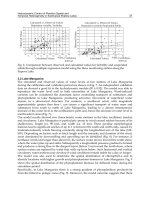
Fig. 1. A) Aerial view of Cesenatico. The bullets represent the position of the sample in Fig.
1B: from the city centre to the sea, respectively: Mariner
Museum, Garibaldi Bridge, Vincian
Ports and sea mouth. B) Salinity and oxygen profiles inside the harbour canal in the position
plotted in nearby Fig. 1A.
20,0
25,0
30,0
35,0
40,0
45,0
50,0
0 20 40 60 80 100 120 140 160 180 200 220 240 260 280 300 320 340
DEPTH (cm)
SALINITY (g/l)
3,0
4,0
5,0
6,0
7,0
8,0
9,0
OXYGEN
(
m
g
/l
)

sea mouth
vincian ports
Garibaldi bridge
Garibaldi bridge
vincian ports
sea mouth
marinery museum
marinery museum

Hydrodynamics – Natural Water Bodies
134
Other research activities, carried out on freshwater-sea water balance for the volumes of
channels of the Cesenatico Port Canal system, (Mancini, 2008) indicated that wastewater,
discharged in the internal zone, has a hydraulic retention time before sea dispersion,
ranging between 1 and 3 days. As a consequence, there is a freshwater storage in the most
internal parts of the channel during incoming tidal phases; on the other side during the
outgoing tidal phases, there is the outflow of the main part of the internal storage
freshwater. Fig. 2B shows monitoring data in correspondence with an internal channel
section at 4 Km from the mouth. The selected section balance between saline waters
introduced by tidal oscillations combined with wastewater flux incoming from inland
maintains the salinity range within a 0-3 g/l. The figure also plots oxygen and redox,
showing similar behaviour.


A

B
Fig. 2. A) Cesenatico northern coastal area characterized by submerged breakwaters. B)
Daily behaviour of physical-chemical parameters measured in the internal section of the
channel limiting transition volumes.

Before the outfall these outgoing volumes flow through the historical tract of the harbour
which presents depths varying between 3 to 5 m. In this tract a typical overflowing volume
upon the static higher density deep layers (Fig. 1B) can be observed. The Marinery Museum
OXYGEN - SALINITY - REDOX
Visdomina bridge - measurements 19.07.07
0,0
4,0
8,0
12,0
16,0
20,0
24,0
28,0
32,0
36,0
40,0
0.00 2.24 4.48 7.12 9.36 12.00 14.24 16.48 19.12 21.36 0.00
hours
redox
mV
0,0
2,0
4,0
6,0
8,0
10,0
12,0
14,0
16,0
18,0

20,0
oxygen
mg/l
- salinity
g/l
redox
salinity
oxygen

Freshwater Dispersion Plume in the Sea: Dynamic Description and Case Study
135
and Garibaldi Bridge are located in the canal, approx. 500 m from the mouth, the Vincian
Ports are located 50 m from the sea mouth. In the last tract close to the mouth a partial
mixing with sea water is permitted, that increases salinity, oxygen and pH, according to the
external sea conditions.
4. Plume modelling on Cesenatico (Italy) discharging area
The hydrodynamic model described above has been used to simulate the evolution of the
plume originating from the freshwater discharge from the harbour canal. The bathymetry
and the geometry of the breakwaters and structures were modelled by a small mesh
dimension. The regular mesh, shown in Fig. 3, was made by 144x170 grid points, with cell
dimensions 12 m x 12 m. On the same figure it is possible to recognize the shoreline, the
harbour canal (points P2, P3 and P4) and coastal defence structures, parallel to the shoreline.
The points on the same Fig. 3 are the profile points where measurements, later described,
have been carried out.




Fig. 3. Investigation area, calculation mesh utilized in model simulations and location of the
fixed investigated points.

Hydrodynamics – Natural Water Bodies
136



Fig. 4A. Example of simulation results of the freshwater plume dispersion in different tidal
phases plotted in Fig. 4B.
0 200 400 600 800 1000 1200 1400 1600
0
200
400
600
800
1000
1200
1400
1600
1800
2000

3h
[m]

[m]
5
10
15
20
25

30
0 200 400 600 800 1000 1200 1400 1600
0
200
400
600
800
1000
1200
1400
1600
1800
2000

[m]
6h

[m]
5
10
15
20
25
30
35
0 200 400 600 800 1000 1200 1400 1600
0
200
400
600

800
1000
1200
1400
1600
1800
2000

[m]
9h

[m]
5
10
15
20
25
30
0 200 400 600 800 1000 1200 1400 1600
0
200
400
600
800
1000
1200
1400
1600
1800
2000

[m]
12h

[m]
5
10
15
20
25
30
0 200 400 600 800 1000 1200 1400 1600
0
200
400
600
800
1000
1200
1400
1600
1800
2000

[m]
15h

[m]
0 200 400 600 800 1000 1200 1400 1600
0

200
400
600
800
1000
1200
1400
1600
1800
2000

[m]
18h

[m]
5
10
15
20
25
30
5
10
15
20
25
30