Hydrodynamics Optimizing Methods and Tools Part 8 ppt
Bạn đang xem bản rút gọn của tài liệu. Xem và tải ngay bản đầy đủ của tài liệu tại đây (3.33 MB, 30 trang )
24 Will-be-set-by-IN-TECH
X
Y
0 0.2 0.4 0.6 0.8 1
0
0.2
0.4
0.6
0.8
1
(a) Isolines of stream function (n = 2250)
X
Y
0 0.2 0.4 0.6 0.8 1
0
0.2
0.4
0.6
0.8
1
(b) Isobars (n = 2250)
X
Y
0 0.2 0.4 0.6 0.8 1
0
0.2
0.4
0.6
0.8
1
(c) Isolines of stream function (n = 3000)
X
Y
0 0.2 0.4 0.6 0.8 1
0
0.2
0.4
0.6
0.8
1
(d) Isobars (n = 3000)
X
Y
0 0.2 0.4 0.6 0.8 1
0
0.2
0.4
0.6
0.8
1
(e) Isolines of stream function (n = 3500)
X
Y
0 0.2 0.4 0.6 0.8 1
0
0.2
0.4
0.6
0.8
1
(f) Isobars (n = 3500)
Fig. 17. Flow picture in the driven cavity (n = 2250, 3000, 3500)
198
Hydrodynamics – Optimizing Methods and Tools
Convergence Acceleration of Iterative Algorithms for Solving Navier–Stokes Equations on Structured Grids 25
X
Y
0 0.2 0.4 0.6 0.8 1
0
0.2
0.4
0.6
0.8
1
(a) Isolines of stream function (n = 5000)
X
Y
0 0.2 0.4 0.6 0.8 1
0
0.2
0.4
0.6
0.8
1
(b) Isobars (n = 5000)
X
Y
0 0.2 0.4 0.6 0.8 1
0
0.2
0.4
0.6
0.8
1
(c) Isolines of stream function (n = 10000)
X
Y
0 0.2 0.4 0.6 0.8 1
0
0.2
0.4
0.6
0.8
1
(d) Isobars (n = 10000)
Fig. 18. Flow picture in the driven cavity (n = 5000, 10000)
7. Acknowledgements
Work supported by Russian Foundation for the Basic Research (project no. 09-01-00151).
I wish to express a great appreciation to professor M.P. Galanin (Keldysh Institute of
Applied Mathematics of Russian Academy of Sciences), who have guided and supported the
researches.
8. Conclusion
«Part of pressure» (i.e. sum of the «one-dimensional components» in decomposition (10)) can
be computed using the simplified (pressure-unlinked) Navier–Stokes equations in primitive
variables formulation and the mass conservation equations. «One-dimensional components
of pressure» and corresponding velocity components are computed only in coupled manner.
As a result, there are not pure segregated algorithms and pure density-based approach
on structured grids. Proposed method does not require preconditioners and relaxation
199
Convergence Acceleration of Iterative Algorithms
for Solving Navier–Stokes Equations on Structured Grids
26 Will-be-set-by-IN-TECH
parameters. Pressure decomposition is very efficient acceleration technique for simulation
of directed fluid flows.
9. References
Barton I.E. (1997) The entrance effect of laminar flow over a backward-facing step geometry,
Int. J. for Num. Meth. in Fluids, Vol. 25, pp. 633-644.
Benzi, M.; Golub, G.H.; Liesen, J. (2006) Numerical solution of saddle point problems, Acta
Numerica, pp. 1-137.
Briley, W.R. (1974) Numerical method for predicting three-dimensional steady viscous flow in
ducts, J. Comp. Phys., Vol. 14, pp.8-28.
Gartling D. (1990) A test problem for outflow boundary conditions-flow over a
backward-facing step, Int. J. for Num. Meth. in Fluids, Vol. 11, pp. 953-967.
Ghia, U.; Ghia, K.N.; Shin, C.T. (1982) High-Re solutions for incompressible flow using the
Navier-Stokes equations and a multigrid method, J. Comp. Phys., Vol. 48, pp.387-411.
Gresho, P.M.; Gartling, D.K.; Torczynski, J.R.; Cliffe, K.A.; Winters, K.H.; Garratt, T.G.; Spence,
A.; Goodrich, J.W. (1993) Is a steady viscous incompressible two-dimensional flow
over a backward-facing step at Re=800 stable? Int. J. for Num. Meth. in Fluids, Vol. 17,
pp. 501-541.
Keskar, J.; Lin, D.A. (1999) Computation of laminar backward-facing step flow at Re=800 with
a spectral domain decomposition method, Int. J. for Num. Meth. in Fluids, Vol. 29,
pp. 411-427.
Martynenko, S.I. (2006) Robust Multigrid Technique for black box software, Comp. Meth. in
Appl. Math., Vol. 6, No. 4, pp.413-435.
Martynenko, S.I. (2009) A physical approach to development of numerical methods for solving
Navier-Stokes equations in primitive variables formulation, Int. J. of Comp. Science and
Math., Vol. 2, No. 4, pp.291-307.
Martynenko, S.I. (2010) Potentialities of the Robust Multigrid Technique, Comp. Meth. in Appl.
Math., Vol. 10, No. 1, pp.87-94.
Vanka S.P. (1986) Block-implicit multigrid solution of Navier–Stokes equations in primitive
variables, J. Comp. Phys., Vol. 65, pp.138-158.
Wesseling, P. (1991) An Introduction to Multigrid Methods, Wiley, Chichester.
200
Hydrodynamics – Optimizing Methods and Tools
10
Neural Network Modeling of
Hydrodynamics Processes
Sergey Valyuhov, Alexander Kretinin and Alexander Burakov
Voronezh State Technical University
Russia
1. Introduction
Many of the computational methods for equation solving can be considered as methods of
weighted residuals (MWR), based on the assumption of analytical idea for basic equation
solving. Test function type determines MWR specific variety including collocation methods,
least squares (RMS) and Galerkin’s method. MWR algorithm realization is basically reduced
to nonlinear programming which is solved by minimizing the total equations residual by
selecting the parameters of test solution. In this case, accuracy of solving using the MWR is
defined by approximating test function properties, along with degree of its conformity with
its initial partial differential equations, representing a continuum solution of mathematical
physics equations.
On fig. 1, computing artificial neural network (ANN) is presented in graphic form,
illustrating process of intra-network computations. The input signals or the values of input
Fig. 1. Neural network computing structure
Hydrodynamics – Optimizing Methods and Tools
202
variables are distributed and "move" along the connections of the corresponding input
together with all the neurons of hidden layer. The signals may be amplified or weakened by
being multiplied by corresponding coefficient (weight or connection). Signals coming to a
certain neuron within the hidden layer are summed up and subjected to nonlinear
transformation using so-called activation function. The signals further proceed to network
outputs that can be multiple. In this case the signal is also multiplied by a certain weight
value, i.e. sum of neuron output weight values within the hidden layer as a result of neural
network operation. Artificial neural networks of similar structure are capable for universal
approximation, making possible to approximate arbitrary continuous function with any
required accuracy.
To analyze ANN approximation capabilities, perceptron with single hidden layer (SLP) was
chosen as a basic model performing a nonlinear transformation from input space to output
space by using the formula (Bishop, 1995):
0
11
(,)
q
n
ii ijj
ij
y
vf b wx b
wx , (1)
where
n
xRis network input vector, comprised of
j
x
values; q – the neuron number of the
single hidden layer;
s
wR– all weights and network thresholds vector;
i
j
w– weight
entering the model nonlinearly between
j-m input and i-m neuron of the hidden layer;
i
v –
output layer neuron weight corresponding to the
i-neuron of the hidden layer;
0
,
i
bb–
thresholds of neurons of the hidden layer and output neuron;
f
σ
– activation function (in our
case the logistic sigmoid is used). ANN of this structure already has the universal
approximation capability, in other words it gives the opportunity to approximate the
arbitrary analog function with any given accuracy. The main stage of using ANN for
resolving of practical issues is the neural network model training, which is the process of the
network weight iterative adjustment on the basis of the learning set (sample)
,, , 1, ,
n
ii i
yikxxR in order to minimize the network error – quality functional
1
() (,)
k
i
JQfi
ww, (2)
where
w – ANN weight vector;
2
(,) ,Q
f
i
f
i
ww– ANN quality criterion as per the i-
training example;
,,
ii
f
i
yy
wwx
–
i-example error. For training purposes the
statistically distributed approximation algorithms may be used based on the back error
propagation or the numerical methods of the differentiable function optimization.
2. Neuronet’s method of weighted residuals for computer simulation of
hydrodynamics problems
Let us consider that a certain equation with exact solution ()
y
x
() 0Ly (3)
for non-numeric value
y
s
equation (3) presents an arbitrary x
s
within the learning sample.
We have
L(y)=R with substitution of approximate solution (1) into equation (3), with R as
equation residual.
R is continuous function R=f(w,x), being a function of SLP inner
Neural Network Modeling of Hydrodynamics Processes
203
parameters. Thus, ANN training under outlet functional is composed of inner parameters
definition using trial solution (1) for meeting the equation (3) goal and its solution is realized
through the corresponding modification of functional quality equation (2) training.
Usually total squared error at net outlets is presented as an objective function at neural net
training and an argument is the difference between the resulted ‘
s’ net outlet and the real
value that is known a priori. This approach to neural net utilization is generally applied to
the problems of statistical set transformation along with definition of those function values
unknown a priori (net outlet) from argument (net inlet). As for simulation issues, they refer
to mathematical representation of the laws of physics, along with its modification to be
applied practically. It is usually related to necessity for developing a digital description of
the process to be modeled. Under such conditions we will have to exclude the a priori
known computation result from the objective function and its functional task. Objective
function during the known law simulation, therefore, shall only be defined by inlet data and
law simulated:
2
1
2
ss
S
Eyf
x . (4)
Use of neuronet’s method of weighted residuals (NMWR) requires having preliminary
systematic study for each specific case, aimed at: 1) defining the number of calculation
nodes (i.e. the calculation grid size); 2) defining number of neurons within the network,
required for obtaining proper approximation power; 3) choosing initial approximations for
training neural network test solution ; 4) selecting additional criteria in the goal function for
training procedure regularization in order to avoid possible solution non-uniformity; 5)
analyzing the possibilities for applying multi-criteria optimization algorithms to search
neural network solution parameters (provided that several optimization criteria are
available).
Artificial neural network used for hydrodynamic processes studying is presented by two
fundamentally different approaches. The first is the NMWR used for direct differential
hydrodynamics equations solution. The NMWR description and its example realization for
Navier-Stokes equations solution is presented in papers (Kretinin, 2006; Kretinin et al.,
2008). These equations describe the 2D laminar isothermal flow of viscous incompressible
liquid. In the paper (Stogney & Kretinin, 2005), the NMWR is used for simulating flows
within a channel with permeable wall. Neural network solution results of hydrodynamic
equations for the computational zone consisting of two sub-domains are presented below.
One is rotating, while another is immobile. In this case, for NMWR algorithm realization
specifying the conjugate conditions at the two sub-domains border is not required.
In the second approach, neural network structures are applied to computational experiment
results approximation obtained by using traditional methods of computational
hydrodynamics and for obtaining of hydrodynamic processes multifactor approximation
models. This approach is illustrated by hydrodynamics processes neural network modeling
in pipeline in the event of medium leakage through the wall hole.
2.1 NMWR application: Preliminary studying
There are specific ANN training programs such as STATISTICA NEURAL NETWORKS or
NEURAL TOOLBOX in the medium of MATLAB, adjusting the parameters of the network
Hydrodynamics – Optimizing Methods and Tools
204
to the known values of the objective function within the given points of its definitional
domain. Using these packages in our case, therefore, does not seem possible. At the same
time, many of optimization standard methods work well for ANN training, e.g. the
conjugate gradients methods, or Newton, etc. To solve the issue of ANN training, we shall
use the Russian program IOSO NS 1.0 (designed by prof. I.N. Egorov (Egorov et al., 1998),
see www.IOSOTech.com) realizing the algorithm of indirect optimization method based on
self-organizing. This program allows minimizing the mathematical model given
algorithmically and presented as “black box”, i.e. as external file module which scans its
values from running variable file generated by optimization program, then calculates
objective function value and records it in the output file, addressed in turn by optimization
program. It is therefore sufficient for computer program forming, realizing calculations
using the required neural network, where the input data will be network internal
parameters (i.e. weights, thresholds); on the output, however, there’ll be value of required
equation sum residual based on accounting area free points. Let us suppose that the
objective function
2
y
x is determined within the interval
0;1
. It is necessary to define
parameters of ANN perceptron type with one hidden layer, consisting of 3 neurons to draw
the near-objective function with given accuracy, computed in 100 accounting points
i
x
evenly portioned in determination field. Computer program for computing network sum
residual depending on its parameters can be as follows (Fortran):
dimension x(100),y(100)
dimension vs(10)
common vs
c vs- values of ANN internal parameters
open(1,file='inp')
read(1,*)vs
close(1)
c 'inp'- file of input data,
c generated by optimization program
do i=1,100
x(i)=(i-1)/99.
end do
c calculation by subprogram ANN ynet
c and finding of sum residual del
del=0.
do i=1,100
y(i)=ynet(x(i))
del=del+(y(i)-x(i)**2)**2
end do
c 'out'-file of value of the minimization function ,
c sent to optimization program
open(2,file='out')
write(2,*)del
close(2)
end
function ynet(t)
dimension vs(10),w(3),b(3),v(3),t1(3),q(3)
Neural Network Modeling of Hydrodynamics Processes
205
common vs
c w-weights between neuron and input
c b-thresholds of neurons
c v-weights between neuron and output neuron
c bv-threshold of output neuron
do i=1,3
w(i)=vs(i)
b(i)=vs(i+3)
v(i)=vs(i+6)
end do
bv=vs(10)
vyh=0.
do i=1,3
t1(i)=w(i)*t-b(i)
q(i)=1./(1.+exp(-t1(i)))
vyh=vyh+v(i)*q(i)
end do
ynet=vyh-bv
end
With IOSO NS 1.0, ANN internal parameter values were obtained with sum residual there
were received the values of the internal parameters of the ANN, giving the sum
0.000023
E (fig. 2).
Fig. 2. Results of using IOSO NS 1.0 for the ANN training
Hydrodynamics – Optimizing Methods and Tools
206
Hence we have neural network approximation for given equation, which can be presented
by the formula
1.954913 0.983267 5.098 0.108345 2.532 0.75393
111
13.786 3.95569 28.3978 3.7751
111
xxx
y
eee
(5)
Using nonlinear optimization universal program products for ANN training is limited to
neural networks of the simplest structure, for dimension of optimization tasks solved by
data packages does not normally exceed 100; however, it frequently forms 10-20
independent variables due to the fact that efficiency of neural network optimization
methods generally falls under the greater dimensions of the nonlinear programming free
task. On the other hand, the same neural network training optimization methods prove
efficient under much greater dimensions of vector independent variables. Within the
framework of given functioning, the standard program codes of neural network models are
applied, using the well-known optimization procedures, e.g. Levenberg-Markardt or
conjugate gradients - and the computing block of trained neural network with those
obtained by the analytical expressions for objective function of the training anti-gradient
components, which in composition of the equation under investigation acts as a "teacher" is
designed.
2.2 Computing algorithm of minimization of neural network decision
Let us consider perceptron operation with one hidden layer from N neuron and one output
(1). As training objective function, total RMS error (4) will be considered. The objective
function shall be presented as a complex function from neural network parameters;
components of its gradient shall be calculated using complex function formula. Network
output, therefore, is calculated by the following formula:
ss
jj
j
yw
xx, (6)
where x - vector of inputs,
s - number of point in training sample, (x) - activation function,
w
j
- weights of output neuron, j - number of neuron in hidden layer. For activation
functions, logistic sigmoid will be considered
,
1
1
jj
j
tb
e
x
x . (7)
Here
b
j
- threshold of j-number neuron of hidden layer; the function t
j
(x,b
j
) , however, has
form of
,
jj
i
j
i
j
i
tb vxb
x , where v
i
- neuron weight of hidden layer.
While training on each iterations (the epoch) we shall correct the parameters of ANN
toward the anti-gradient of objective function -
E(v,w,b), which components are presented
in the following form:
,
s
sss
jj
ij
E
byf
w
xx; (8)
Neural Network Modeling of Hydrodynamics Processes
207
,1 ,
s
ss s s s
jj j j j
i
ij
E
yf
wb bx
v
xx x; (9)
,1 ,
s
ss s s
jj j j j
j
E
yf
wb b
b
xx x. (10)
Thereby, we have got all the components of the gradient of the objective function of
minimization, comparatively which iterations will be consecutively realized in accordance
with the general formula
E
ww. (11)
Here
w is vector of current values of network weights and thresholds.
3. Using NMWR for hydrodynamics equations solving
Parameter optimization of neural network trial solutions is achieved by applying several
optimization strategies and by subsequently choosing the maximum effective one (see
Cloete & Zurada, 2000). First strategy is to apply totality of effective gradient methods
"starting" from various initial points. The other strategy is to apply structural-parametrical
optimization to ANN training; this method is based on indirect statistic optimization
method on self-organizing basis or parameter space research (see: Egorov et al., 1998;
Statnikov & Matusov, 1995).
Any versions for multi-criterion search of several equations system solution are based on
different methods of generating multiple solutions, satisfying Pareto conditions. Choosing
candidate solution out of Pareto-optimal population must be based on analysis of
hydrodynamic process and is similar to identification procedure of mathematical model. In
any case, procedure of multi-criterion optimization comes to solving single-criterion
problems, forming multiple possible solutions. At the same time particularities of some
computational approaches of fluid dynamics allows using iteration algorithms, where on
each step solution at only one physical magnitude is generated.
3.1 Modeling flows – the first step
The computational procedure described below is analogous to MAC method (Fletcher,
1991), investigating possibility of NMWR application based on neural net trial functions.
Laplace equation solution
Computational capabilities of the developed algorithm can be illustrated by the example of
the solution of Navier-Stokes momentum equations, describing two-dimensional isothermal
flows of viscous incompressible fluid. On the first stage we will be using this algorithm for
Laplace equation solution
22
22
0
xy
. (12)
Let us consider the flow of incompressible fluid in the channel (fig. 3).
Hydrodynamics – Optimizing Methods and Tools
208
0
y
1
y
0
x
0
y
0
2
2
2
2
yx
x
y
Fig. 3. Computational area
Here’s how the boundary conditions are defined: on solid walls u=v=0, on inflow boundary
u=0, v=1, on outflow boundary
0
uv
xx
. There are no boundary conditions for pressure
except for one reference point, where p=0 is specified (in the absolute values p=p
0
),
considering which indication of incoming into the momentum equation
p
x
and
p
y
is
realized.
For solving flow equations by predictor method it is necessary to specify initial velocity
distribution within the computational area, satisfying the equation of continuity. For this
purpose, velocity potential
,x
y
is introduced and
u
x
and v
y
. As a result of
Laplace equation solution, velocity distribution is generated, which can be indicated as free-
vortex component of the sought quantity.
If the result of learning sample neuronet calculations is defined by the following formula
ss
jj
j
vf
xx, where
,
T
x
y
x -input variables vector, s - point number in the
learning sample,
f х - activation function,
j
v
- output neuron weights, j - neuron number
in the hidden layer as activation function the logistical sigmoid is used
,
1
1
jj
j
tb
f
e
x
x
,
where
j
b - threshold of the j-number neuron hidden layer, and the function
,
jj
tbx looks
like
,
jj
i
j
i
j
i
tb wxb
x where
i
j
w - hidden layer neurons weights, then analytical
expressions for the second speed potential derivatives can be calculated using the following
formula
2
223
2
,3 ,2 ,
sss
jij j j j j j j
s
j
i
vw f b f b f b
x
xxx. (13)
Neural Network Modeling of Hydrodynamics Processes
209
Equation summary residual with substituted trial solutions (1) on arbitrary calculation area
points with coordinates х
s
with expressions application (13) can also be calculated
analytically
22
222
222
11
22
sss
si s
i
E
xxy
. (14)
Therefore, trial solution (1) training problem of neural network equation consists in SLP
hidden layer parameter selection (weights and thresholds) at which the summary residual
(14) has the minimal value limited to zero. The computer program described above, with
training procedure target function being set functionally by applying analytical expressions
for second derivatives
2
2
x
and
2
2
y
, is used for parameter adjustment of learning model.
Efficiency of searching of neuronet learning solution parameters depends on problem
dimension, i.e. weights and perceptron thresholds variable adjusted quantity. The more
significant is neurons quantity in trial solution, the higher is ANN approximate capacity;
however, achieving high approximation accuracy is more complicated. At the same time,
neuron quantity depends not only on simulated function complexity, but also on calculation
nodes quantity in which the residual equation is calculated. It is known that generally
points’ quantity increase in statistical set used for neural network construction is followed
by increase in necessary neurons network (Galushkin, 2002; Galushkin, 2007) quantity.
Consequently, the dense calculation grids application results in nonlinear programming
problems; while applying rare calculation grids, it is necessary to check the solution
realization between calculation nodes, i.e. there is a problem of learning solution procedure
standardization. In the neuronet solution reception context on known equation, it is
convenient using traditional additive parameter of training neural model quality - a control
error which is calculated on the set of additional calculation nodes between calculation grid
nodes. Number of these additional calculation grid nodes can be much more significant, and
they should cover the whole calculation area, because the nodes number increase with
control error on known network parameters does not result in essential computing expenses
growth. Hence, referring to learning solution neuronet parameters reception, there exists an
issue of solving twice-criterion problem of nonlinear optimization along with minimizing
simultaneously both summary residual in control points, or the control error can appear as a
restriction parameter, in the limited set of calculation nodes and in this case the neural
network solution parameters reception is reduced to the conditional nonlinear optimization
problem.
At the first stage, residual distribution of the current equation (5) on various calculation
nodes and the corresponding speed vector distribution
,
T
uvv , where speed nodes
u
x
and v
y
. As a whole, the received neural network solution satisfies the equation
(5) except for calculation nodes group, for example, in the input border right point vicinity,
due to a sudden change of the boundary conditions in this point. In areas with the solution
insufficient exactness we will place the calculation nodes additional quantity using the
Hydrodynamics – Optimizing Methods and Tools
210
following algorithm. Let us formulate the Cohonen neural network with three inlet variables
presented by the coordinates of available computation nodes x and y, and also the equations
(5) residual value in these nodes, along with the required cluster centers quantity equal to
the additional nodes quantity. The cluster center coordinates which will generally be placed
in areas with the learning solution low precision (Prokhorov et al., 2001) we will consider
additional computation nodes coordinates. The number of these additional nodes in each
case is different and defined by iterations, until the decision error does not accept
comprehensible value. As a result of the additional formation of received neural network
learning solution using additional computation nodes, it turned out to be possible to
increase the solution local accuracy in the point B vicinity while maintaining the accuracy
high in all other points.
Fig. 4. Formation of additional computation nodes for Laplace equation solution
Therefore, not only has the computing experiment proven reception opportunity of the
general neural network solution in the calculation area, but also defined coordinate
calculation logic of computational nodes for increasing the accuracy of neural network
initial equation solution. Let us study a reception opportunity of the Poisson equation
solution using an irregular computational grid, i.e. equation total residual with solutions (1)
will be calculated in nodes located in the casual image or certain algorithm, which use has
not been connected with the necessity of computational grid coordination and
computational area borders.
Poisson equation
Let us study a neural network solution precision on irregular calculation scales for Poisson
equation
22
22
0
pp
xy
. (15)
This equation is particularly used for calculating the pressure distribution as well as for time
iterations organization at the Navier-Stokes equations solution by pseudo-non-stationary
algorithms (Fletcher, 1991). For the solution we shall use an irregular calculation grid,
because, in contrast to fluid dynamics classical numerical methods, it does not result in the
neutral network learning functions algorithm complication. Meanwhile, advantages using
calculation nodes located in calculation area for the complex geometry study current are
obvious. The decision is defined by the equations (15) with the right side as follows
22
22
2
pp
uv vu
x
y
x
y
xy
, (16)
Neural Network Modeling of Hydrodynamics Processes
211
where speed nodes
u
x
also v
y
are received as a result of the Laplace equation
solution (12). Calculation grid points are formed as centers of Cohonen network clusters
constructed on units coordinates of the uniform rectangular scale and on the right part of
the equation (16) corresponding to these units values Δ. Fig. 6 (а) presents formation re sults
of the calculation grid and the speed distribution on the pseudo-non-stationary algorithm
first iterative step of the Navier-Stokes equation solution. Here it was possible to receive an
exact neural network solution for the whole calculation area without using additional set of
calculation nodes.
Let us now study am incompressible fluid internal flow within a channel with a stream
turning (fig. 3). Navier-Stokes equation system describing two-dimensional isothermal flows
of the viscous incompressible fluid (Fletcher, 1991):
0
uv
xy
; (17)
22
22
1
0
Re
p
uu uu
uv
xxy
xy
; (18)
22
22
1
0
Re
p
vv vv
uv
yxy
xy
. (19)
Here u, v – nodes speed, Re - Reynolds number. Hydrodynamics equations system is written
in the non-dimensional view; i.e. it includes non-dimensional values
*
u
u
u
,
*
v
v
u
,
*
r
r
D
,
*
2
p
p
u
, Re
uD
. Quality of u
and any speed and linear size values
can be chosen in the current field, for example an input fluid speed value in the channel and
the channel width
h .
Boundary conditions are stated as follows: on solid walls
u=v=0, on the input border u=0,
v=1
, on the output border
0
uv
xx
. Let us consider that there is rectangular region
[a,b]
[c,d] within the plane XY, and there is a rectangular analytical grid, specified by
Cartesian product of two one-dimensional grids
{x
k
}, k=l,…,n and {y
l
}, l=l,…,m.
We will understand neural net functions
,, ( ,,)
NET
uvp f xy w as the (17)-(19) system solution
giving minimum of the total squared residual in the knot set of computational grid. The trial
solution (fig. 5) of the system (17)-(19)
u, v, p can be presented in the form equation (1):
12
1
(,,) ( )
q
iii i u
i
uxy vfbwxwyb
w ; (20)
2
12
1
(,,) ( )
q
iii i v
iq
vxy vfbwxwyb
w ; (21)
Hydrodynamics – Optimizing Methods and Tools
212
3
12
21
(,,) ( )
q
iii i
p
iq
p
xy vf b w x w y b
w . (22)
Here again, w is the vector of all the weights and thresholds of the net. In this case the
amount of
q neurons in the trial solutions remains the same for each decision variable set.
This is the parameter on which depend approximated capabilities of neural net trial
solution. Result of computational algorithm functioning should be achievement of necessary
accuracy level of solution at
q minimum value.
Fig. 5. Neural net trial solution
Let us name the residuals of equations (17)-(19)
R
1
, R
2
and R
3
correspondingly, then for the
vase of NMWR realization for parameters setup of the trial solution it is necessary to
minimize three objective functions
222
123
;; minRRR . In the simplest case, the only solution
of the multi-criterion problem of minimization can be generated substituting of three
criterions by one, presented in compression form; for example,
2222
123
minRRRR .
Presenting the trial solution in the form of continuous functions (20)-(22) allows to define
analytically the first and the second differential coefficient in the equations (17)-(19),
knowing which one can generate analytic expressions of the function of residuals
R
s
(w,x,y)
and further for antigradient component of the total residual in the
s-reference point at ANN
inner parameters
j
R
v
,
i
j
R
w
and
j
R
b
, being later used in the minimization algorithm in
accordance with anti-gradient direction.
For the momentum equations solution by MAC method, it is necessary to specify an initial
speeds distribution in the calculation area satisfying to the continuity equation. For this
purpose, the speed potential
,xy
is introduced,
u
x
and v
y
. As a Laplace
equation solution result, we obtain speed distribution which can be called non-vortex
required value.Final speeds and pressure distribution are results of the momentum
equations solution according to the following algorithm.
The speed distribution on the following time layer is calculated according to the formula
11nn n
tp
uF
, (23)
where pressure distribution to each iterative step is defined upon the Poisson equation
solution
Neural Network Modeling of Hydrodynamics Processes
213
21
1
(,)
nn
NET
p
fxy
t
F
. (24)
Vector ( , )
T
FGF introduced to this algorithm can be calculated by the momentum
equations (18-19); or Poisson equation (16) can be used for pressure calculation. Thus, the
solution for pressure received from the equation (16) results in the continuity equation
realization at the moment of time 1
n
. Once
1n
p
is calculated, substitution of these
values in the formula
11nn n
tp
uF allows to determine
1n
v
. The iterative process
goes on until speed distribution stops varying.
Let us briefly generalize the above mentioned results of calculation experiment in methodic
form to set dynamic calculation scale at the Navier-Stokes equations (17)-(19) solution by the
establishment method. First, Laplace equation (12) solution is calculated with the received
scale or with rectangular scale, or by means of random numbers generator, or by using the
Sobol - Statnikov generator of
LP
(Statnikov & Matusov, 2002); then, distribution solving
equation residual in the grid nodes; third, the additional multitude of calculation nodes is
generated with using the Cohonen network; then, if the precision is not achieved, points 2
and 3 are realized and the additional calculation components quantity grows until exact
neural network solution for the whole calculation area is found; further, pseudo-non-
stationary algorithm iterations are organized by using the equations (23)-(24) where
equation (16) solution is found on each time step on the multitude of calculation
components, the coordinates of which vary depending on the Poisson equation right part
distribution for each iterative step; finally, at steps 3 and 5 realization of structural
optimization algorithms and learning neural network solutions standardization formation
a)
b)
c)
Fig. 6. Net velocity distribution
Hydrodynamics – Optimizing Methods and Tools
214
stated in (Kretinin et al., 2010). On fig. 6 (а-c), changing dynamics of calculation components
during realizing various moments of time of equations (23)-(24) algorithm is shown, the
speed vector distribution reorganization during the transition from the equation (12)
solution to the equations (17)-(19) solution is also illustrated.
Finally, analytical solution (as neural network function) for Navier-Stokes equations (17)-
(19) systems within the channel with stream turning at Re 100
which is expressed by the
formula (23) on last iterative layer and neural network dependence of the pressure
distribution on this layer
3
12
21
(,,) ( )
q
iii i
p
iq
p
xy vf b w x w y b
w
with weights calculated array and the boundary network w
,,wvb .
3.2 Modeling flows in rotating ring zone - the equations that are applicable to rotating
reference frame
For this flow, NMWR solves conservation equations for mass and momentum describing
incompressible flows of viscous Newtonian fluid.
Continuity equation
0
j
j
u
x
. (25)
Momentum equations
j
i
i
j
i
j
i
jj ijji
u
p
u
uu uu f
xx xxxx
. (26)
For flows in rotating domain (fig. 7), the equations for conservation of mass and momentum
are written for the relative velocity formulation, where
f
i
in right hand side is given by
2
i
f
ur
. (27)
The absolute velocity formulation is used in the non-rotating domain, and
f
i
=0. Thus, the
standard
k
turbulence model is used.
Let us consider the neural network functions
,,, ( ,,)
iNN
upk f xy
w as equations solution,
where w– all weights and network thresholds vector that assure summary quadratic
residuals minimums for each equation in optional totality of computation nodes
coordinating each neural network solution learning iteration, are generated using the
random number generator.
Neuronet learning solution parameter search process efficiency depends on problem
dimension, i.e. weights and perceptron thresholds varying adjusted quantity. The more
significant is neurons quantity in trial solution, the higher is ANN approximate capacity;
however, achieving high approximation accuracy is more complicated.
Neural Network Modeling of Hydrodynamics Processes
215
Fig. 7. Rotating Domain
At the same time, neuron quantity depends not only on simulated function complexity, but
also on calculation nodes quantity in which the residual equation is calculated. It is known
that generally points’ quantity increase in statistical set used for neural network
construction is followed by increase in necessary neurons network (Galushkin, 2002;
Galushkin, 2007) quantity. Consequently, the dense calculation grids application results in
nonlinear programming problems; while applying rare calculation grids, it is necessary to
check the solution realization between calculation nodes, i.e. there is a problem of learning
solution procedure standardization. In the neuronet solution reception context on known
equation, it is convenient using traditional additive parameter of training neural model
quality - a control error which is calculated on the set of additional calculation nodes
between calculation grid nodes. The number of these additional calculation grid nodes can
be much more important and they should cover all calculation area because the nodes
number increase in which the control error on known network parameters does not result in
essential computing expenses growth. Hence, at the learning solution neuronet parameters
reception there is a problem of solving the multi-criterion problem of the nonlinear
optimization and to minimize simultaneously both the summary residual in control points,
or the control error can appear as a restriction parameter, in the limited set of calculation
nodes and in this case the neural network solution parameters reception is reduced to the
conditional nonlinear optimization problem.
On figure 8, velocity distribution vector within the current random computation nodes of
revolving ring on one of neural network training iteration of equation (25)-(26) decisions is
presented. Contours of stream function within the computational zone obtained by using
NMWR are presented on fig. 9.
Hydrodynamics – Optimizing Methods and Tools
216
Fig. 8. Velocity distribution on one of neural network training iteration
Fig. 9. The contours of stream function
Neural Network Modeling of Hydrodynamics Processes
217
4. Modeling leakage in a fuel transfer pipeline
Method of leakage zonal location (Zverev & Lurie, 2009), which generalizes the known
method of leakage detection by hydraulic gradient line salient point, can be used to define of
pipeline leakage position. When using the “base” zone location method variant, it is supposed
that in case of stationary process, hydraulic gradients
1
i and
2
i before and after the leakage are
constant and can be designed by the known values of liquid charge at the ends of controllable
site. I.e., the distribution indignation of hydrodynamic parameters is not taken into account in
comparison with the established flow which arises because of the environment outflow
influence through the leakage aperture. It results in speed profile deformation within the cross
sections of the pipeline near the leakage and the nonlinear dependence of hydraulic gradient
in the function of distance from position of leakage downwards the stream. In order for pipe
cross section speed distribution of the pipe to become appropriate for the established flow,
the distance up to 40-60 calibres from leakage coordinate
у
x
can be required. Defining
nonlinear dependence of hydraulic gradient function near the leakage is possible either based
on special experimental researches, or based on the numerical decision of hydrodynamics
equations in three-dimensional statement. The given function can be added to the algorithm of
zone location methode to reduce the leakage position coordinate definition error.
One pipeline section of 300 m length and diameter
1mD is used for the nonlinear
dependence of the total pressure drop determination along the pipeline length in the
leakage neighborhood through the wall hole. The leakage position coordinate is
fixed 155.5 m
у
x . On the segment
140,200 mx
computational faces are formed with an
interval
1hm . In segments
100,140 mx and
200,250 mx computational faces are
disposed with an interval
10 mh
. Such a leakage location (approximately in the middle of
the pipeline sector into a question) and computational faces disposition have been chosen
for the influence elimination of the boundary conditions setting in the computational zone
inlet and outlet on the flow distribution near leakage position. The leakage hole
l
DD
relative diameter during the computational planed experiment is constant. The
mathematical model includes conservation equations for mass and momentum enclosed by
the standard
k
turbulence model. The local hydraulic friction coefficient in any section
of the pipeline is defined by the ratio
2
8
rR
u
r
u
, (27)
where
2
0
1
2
R
uurdr
R
- design section average speed,
- dynamic factor of liquid viscosity.
Turbulent flow speed distribution within the pipe cross section is described by the universal
logarithmic dependence
log
uy
u
AB
u
, (28)
where
8
uu
- the dynamic speed, y - the distance from the wall,
- the kinematic
viscosity.
Hydrodynamics – Optimizing Methods and Tools
218
At the statement of boundary conditions on the input, mass charge
1
m
or the speed
1
u
appropriate to this charge is set. In the grid units belonging to the leakage aperture,
liquid outflow speed
у
u
is appointed. The given parameter at numerical researches varies
for the modeling leakages of various intensity. For any point of the calculating area, any
operational value of pressure
x
of all the hydrodynamical parameters are equaled to
zero, for the concerning of which differences of pressure will be calculated, is set. On the
output from the calculating area the conditions of the established current are set, i.e. the
derivatives modeling of the boundary layer the standard wall functions for parameters of
turbulence k and ε (Fletcher, 1991) are used.
The equations discretization is effectuated on the base of finite volumes method in the
combination with hexagonal grid. On fig. 10 the formation of the grid in the calculating
sections of the pipeline is represented.
Fig. 10. Calculation grid in the pipeline sections
4.1 The plan of computing experiment
If
12
,xx are the coordinates of the beginning and the end of the controllable pipeline sector,
then
12
,ii are hydraulic gradients before and after the leakage respectively,
0
p
is total
pressure drop of the sector, so in case of
1
iconst
from the beginning of the sector to the
leakage and
2
iconst from the leakage up to the end of the sector, in the stationary
hydrodynamic mode, leakage coordinate shall be defined by the formula
Neural Network Modeling of Hydrodynamics Processes
219
01122
12
у
pg
ix ix
x
gi i
. (29)
Let us present the total pressure drop nonlinear dependence for its calculation in leakage
neighbourhood in nonlinear function form
12
,,
i
NN NN
if iixx
on the pipeline sector
,
NN NN NN
xx x l
, where for our computational model the left area limit coordinate of the
nonlinear leakage function determination
150 m
NN
x
and the determination length
fragment area
60 m
NN
l
(leakage is situated in the point with coordinate
155,5 m
у
x
).
In this case, total pressure drop in the controlled sector
12
,xx
is calculated by the
following formula
0
1122 12
0
,,
NN
l
i
NN NN NN NN NN
p
ix x ix x l
f
iix x dx
g
. (30)
In the known function
12
,,
i
NN NN
fiixx , the present equation is nonlinear with one
unknown value
NN
x
. After solving this equation, we can define the pipeline leakage
coordinate
l
x .
Starting from above-mentioned, computational experiment is effectuated with the
purpose of function determination
12
,,
i
NN NN
fiixx , i.e. the total pressure drop
dependence in the leakage neighbourhood
i (criterion) of three variables
11
NN
i
g
i
,
221
/
NN
iii
and
NN NN
xxx
(factors). Earlier, the interval forfactor variation
0,60
NN
x
was determined. Let us determine the intervals
1
10,20
NN
i ,
2
0,5,0,95
NN
i . The plan of computing experiment is made with the points received with
the help of Sobol-Statnikov generator of quasiuniform number sequences (Statnikov &
Matusov, 2002). The working hypercube of space
R
3
is filled with the points
12
,,
NN NN
NN
ii x
according to
LP
algorithm (Statnikov & Matusov, 2002). Choice of this
algorithm for the experiment plan formation is made by high efficiency of the research
method of parameter space based on the sounding of computational area by points of the
uniform distributed sequence.For each variable, parameter combinations
12
,
NN NN
ii from
the experiment plan limitation boundary conditions in the computational model are
selected by determining values corresponding tothe inlet mass flow
in
m
and leakage
intensity
l
m
, where the hydraulic friction coefficient is calculated by the implicit formula
of Altschul for "smooth" pipes
12,82
2,04log
Re
.
As a result of computational hydrodynamics equations decision, we obtain the value
distribution of total pressure drop on the length of the controlled pipeline sector, from
which we are exterminating the criteria value
i for the corresponding value
NN
x
from the
experiment plan. Let us now register the obtained vector
12
,, ,
NN NN
NN
ii xi in database for
the posterior generation of neural network dependence
12
,,
iNNNN
NN NN
if i i x
.
For the illustration of numerical calculations, the distribution of speed in the leakage
neighbourhood is presented on Fig. 11, and on fig. 12 the distribution of the hydraulic
gradient on the pipeline sector
100,250 mx
for factor values
1
Pa
14
m
NN
i
,
221
/ 0,5;0,57;0,64;0,71;0,8;0,9
NN
iii
is presented.
Hydrodynamics – Optimizing Methods and Tools
220
Fig. 11. Speed distribution in the leakage neighbourhood
Fig. 12. Total pressure drop distribution for 1 meter of pipeline length
x, m
gi
Neural Network Modeling of Hydrodynamics Processes
221
4.2 The neural network regressive model
For the regressive dependence construction,
12
,,
iNNNN
NN NN
if i i x artificial neural
networks device is used. For the formation of display
12
,,
iNNNN
NN NN
if i i x, the standard
structure of the multilayer perceptron (MLP) with 3 inputs, one output and two latent layers
with 7 and 5 neurons accordingly was used. At training, MLP algorithm of Levenberg-
Markardt was used. The total RMS error on 512 points of statistical sample was
E=0.001.
The comparative analysis of dependences calculation results obtained for inlet parameters
values
1
Pa
16
m
gi
,
2
1
0.9
i
i
is presented on Fig. 13 and
1
Pa
10
m
gi
,
2
1
0.8
i
i
for
0,60 m
NN
x from the differential equation computational solution– continuous lines
and determined with neural network dependence – markers. It is also necessary to note the
high approximation precision.
Fig. 13. Comparative analysis of neural network data and numerical solution results
5. Conclusion
Results presented in this chapter concern one of many applications of neural network
learning functions to the mathematical physics problems solution, which is solution of
hydrodynamics equations. Using learning functions of neural network allows to exclude the
errors in solving differential equations caused by derivatives discretization and the borders
low precision representation. Numerical algorithm of Navier-Stokes equations system
solution differing from known fluid dynamics methods by the possibility of computational
grid arbitrary formationis developed. The formation technique of the additional nodes file
depending on learning solution local accuracy is offered.
NN
x
1
i
i