Modern Telemetry Part 14 pptx
Bạn đang xem bản rút gọn của tài liệu. Xem và tải ngay bản đầy đủ của tài liệu tại đây (3.73 MB, 30 trang )
Modern Telemetry
382
Fig. 9. Digital elevation model of Fig. 10. Depth availability in Round Lake
Round Lake.
Fig. 11. Hardness map of Pigeon River at Fig. 12. Hardness (substrate) availability in
Round Lake obtained from sonar data. Round Lake.
Substrate and Depth: Maximum depth of Round Lake is 16m. A depth map of Round Lake is
shown in Fig. 9. Two deep holes, one off the Northeast corner of each island, are found in
the lake. The general structure is bowl shaped. Depth availability is shown in Fig. 10. Two
and three meters depths are available 33 and 16% respectively. Seven, 8, and 9 meter depths
are available 5, 6, and 8% respectively.
Substrate hardness of the lake is shown in Fig. 11. Substrate was generally related to depth.
The deeper areas of the lake had softer substrates with a high percentage of silt. The shallow
sections along the shoreline to about 10m depth had sandy substrates. Cobble and rock
substrate predominated in areas of high flow at the inlet and outlet. Availability of substrate
hardness was 11, 25, and 17 percent for hardness values of 125 (coarse sand), 130 (gravel),
0
5
10
15
20
25
30
35
123456789101112131415
Depth of Lake (m)
Percent of total available habitat
16m depth
1m depth
Hardness = 150 (Rock)
Hardness = 95 (Clay)
0
5
10
15
20
25
30
95 105 115 125 135 145 155 165
Substrate Hardness
Percent of total Availability
Movements and Habitat Use by Lake Sturgeon (Acipenser fulvescens)
in an Unperturbed Environment: A Small Boreal Lake in the Canadian Shield
383
and 135 (medium sand) respectively (Fig. 12). Substrate hardness of 110 (fine sand) had a
frequency of 16 percent.
Phi Particle Size (mm) Category Hardness
9 <0.0039 clay 95
5,6,7,8 0.0039 – 0.0625 silt 100
4 0.00625 - 0.125 Very fine sand 105
3 0.125 – 0.25 Fine sand 110
2 0.25 – 0.5 Medium sand 115
1 0.5 - 1 Coarse sand 120
0 1 – 2 very coarse sand 125
-1,-2,-3 2 – 16 gravel 130
-4,-5 16 - 64 Pebble 135
-6,-7 64 - 256 Cobble 140
-8 >256 Boulder 145
Table 3. Sediment classification scheme for Round Lake.
Thirty–seven sediment grabs were taken to compare with the hardness values obtained
from the sonic data. Table 3 lists the substrate classification given to each range of hardness
values. Hardness values range from 95 (clay) to 150 (rock, see Fig. 11).
4. Lake sturgeon movements
The biological data for the nine lake sturgeon tagged with acoustic tags are listed in Table 2.
The nine fish were tracked for 27 days and 15,446 locations were obtained. Movements
ranged from individuals that were mostly sedentary to highly mobile individuals. Daily
movements were variable between fish as well as by the same fish on different days. Figure
13 shows the locations of fish 4015 on four separate days. Movement was confined to the
inlet to Round Lake on day 210. Movement increased on days 211 and 212 and covered most
of the lake. Movement on day 220 was restricted to the river outlet.
A comparison of the movements of juvenile and adult lake sturgeon is shown in Fig. 14.
Movements of the juvenile fish were focused at the inlet and outlet and in the deep hole
(~16 m). Movements of the subadult and adult lake sturgeon were also associated with
the inlet and outlet but the movements were more widespread around the lake. The
channel where water entered the lake was a preferred site as was the outlet from the lake.
Figure 15 shows the swimming depth of sturgeon 4014 on day 206 relative to the bottom
depth. Note the day 206 is based on January 1 being day 1. Sturgeon 4014 was on the
bottom 30% of all locations on day 206. During the hours from midnight to 5 AM sturgeon
4014 was in the water column the majority of the time. From 5 AM to 11 PM more time
was spent on the bottom. After 11 PM lakes sturgeon movements shifted to the water
column. Figure 16 shows sturgeon 4015 on day 221 where 53% of all locations were on the
bottom on day 221. Sturgeon 4017 on day 211 was on the bottom for the entire day but
periodically swam to the surface (Fig. 17). Figure 18 shows the overall distribution of each
lake sturgeon fitted with a pressure tag and the total distribution of all fish on the bottom
and in the water column.
Modern Telemetry
384
Fig. 13. Movements of lake sturgeon 4015 on four separate days.
Fig. 14. Comparison of the movements of adult and juvenile sturgeon in Round Lake
Juvenile
Adult Fish
A) Fish 4015, Day 210
C) Fish 4015, Day 212
B) Fish 4015, Day 211
D) Fish 4015 Day 220
Movements and Habitat Use by Lake Sturgeon (Acipenser fulvescens)
in an Unperturbed Environment: A Small Boreal Lake in the Canadian Shield
385
Fig. 15. A comparison of swimming depth Fig. 16. A comparison of swimming depth and
and bottom depth of the lake for bottom depth of the lake for sturgeon 4014 on
sturgeon 4014 on day 206. day 221.
0
10
20
30
40
50
60
70
80
90
100
4014(206) 4015(210) 4017(206) 4017(219)
Lake Sturgeon (day)
Percent of total locations
% on the bottom
% in the water column
Fig. 17. A comparison of swimming depth Fig. 18. Time spent in the water column and on
and bottom depth of the lake for the lake bottom for sturgeon 4014, 4015 and
sturgeon 4017 on day 211. 4017 combined total.
-10
-9
-8
-7
-6
-5
-4
-3
-2
-1
0
6 134 258 414 545 719 824 1000 1148 2149 2321
Time
Depth (m)
Swimming Depth
Bottom Depth
-10
-9
-8
-7
-6
-5
-4
-3
-2
-1
0
6 134 258 414 545 719 824 1000 1148 2149 2321
Time
Depth (m)
Swimming Depth
Bottom Depth
-
-
-
-
-
-
-
-
0
1 31 63 91 120 144 175 2046230
Tim
Depth (m)
Swimming Depth
Bottom Depth
Modern Telemetry
386
Figure 20 shows substrate selection of sturgeon 4014, 4015, 4017 from the 7 day sample.
Substrate with a hardness value of 110 was selected 53% of all locations.
Overall, lake sturgeons were located on the bottom 39% and in the water column 61% of the
locations on the 7 day sample (day 215 based on January 1 being day 1).
The amount of time spent at the surface varied with time of day. The majority of locations
< 1m occurred between the hours of 8 PM and 8 AM (Fig. 19).
The selection of depth was analysed from two perspectives. Figure 21 shows the overall
depth selection of the three lake sturgeon tagged with depth tags. Thirty percent of all
locations were less than two meters. Sixty-six percent were less than four meters. Figure 22
shows the depth selection of the three lake sturgeon including only the locations in which
they were in contact with the substrate during the 7 day sample. Seven, 8, and 9 meter
depths were selected 11, 31, and 21 percent respectively. Figure 23 shows movements of lake
sturgeon 4014. It spent 70% of the time in the water column at the inlet on day 206 and on
day 221 lake sturgeon 4014 spent 47% of the time in the water column.
Figure 24 shows movements of lake sturgeon 4015 on day 210. It spent 59% of its time in the
water column at the inlet of the river. Lake sturgeon 4017 (Fig. 25) spent 60% of the time in
the water column on days 206 and 222, 25% on day 211, and 88% on day 219. On days 211
and 219, sturgeon 4017 covered most of lake, including areas around the inlet and outlet.
The use of depth tags eliminates the guess work of whether a fish was on the bottom or in
the water column at each position. Comparisons were made in this study among telemetry
position, depth and substrate using data from depth tags. Substrate, depth and current were
the three primary environmental variables measured.
Lake sturgeon movements ranged from sedentary to highly active. Movements in the areas
of the inlet and outlet, areas of higher flow rate were quite common as well as movements in
the deeper areas and along the natural flow of the river. Movements along the shorelines
were rare. Along the shorelines the water is shallow, there is little flow, and the substrate is
primarily sandy. Movements of smaller and larger fish were similar but larger fish moved
greater distances. Nevertheless, juvenile fish appear to use most of the same habitat as the
larger fish. Movements for both were related to the inlet and outlet and the deeper part of
the lake.
The larger lake sturgeon spent a significant amount of time in the water column and at the
surface. We do not know what juveniles were doing concerning depth selection because
they were too small to be fitted with tags with pressure sensors. The amount of time in the
water column by the larger fish suggests these fish were feeding on organisms drifting with
the current. A majority of the records on movement were near the inlet and outlet where
drift nets recovered insects and the occasional small fish Extensive lake sturgeon activity
was noted where insects were carried by the current, were floating on the surface, or were
emerging i.e. mayflies. High sturgeon activity in some areas was also correlated with clam
beds.
The timing of movements in the water column and at the surface was correlated to light
intensity. Lake sturgeon spent more time at the surface at night than during the day, when
more time was spent on the bottom.
Based on the comparison of substrate selection and substrate availability lake sturgeon were
found over fine sand, cobble, and rock substrate at higher frequencies than the proportion of
this substrate in the lake. Coarse sand and gravel substrates were selected at a lower
frequency than their proportions in the lake.
Movements and Habitat Use by Lake Sturgeon (Acipenser fulvescens)
in an Unperturbed Environment: A Small Boreal Lake in the Canadian Shield
387
Fig. 19. Day and night comparison of time spent at the surface for sturgeon 4014, 4015, and
4017.
A) 4014, day
B) 4014, night
C) 4015, day
D) 4015, night
E) 4017, day
F) 4017, night
Modern Telemetry
388
Fig. 20. Substrate selection by lake sturgeon in Round Lake (see Table 3)
Fig. 21. Overall depth selection by lake Fig. 22. Depth selection by lake sturgeon when
sturgeon in Round Lake. in contact with the substrate.
Hexagenia (Ephemeridae) is a common prey item of lake sturgeon and silt and clay
substrates are the preferred habitats. By contrast clams were often found in sandy
substrates. While invertebrates were not common in the sieved substrates mayflies are a
major food source for most fish species in the lake. Similarly, mayflies were a major food
item of lake sturgeon, based on stomach contents which was verified by gavage. It appears
in this system that mayflies are a major food source but competition for this food source by
most fish species in the lake may make this food item a potentially limiting factor. Similar
observations have been reported by others (Choudhury et al 1995; Chiasson et al. 1997).
The selection of depth based on horizontal and vertical movements of lake sturgeon seems
to be related to current. Lake sturgeon tended to stay in the water column more often in
areas of high flow such as the inlet and outlet. Since the study took place in mid summer
and this activity was not related to spawning behaviours or movement related to fall/winter
migrations the majority of movements are likely related to feeding behaviour.
0
50
100
150
200
250
300
95 100 105 110 115 120 125 130 135 140 145
Substrate Hardness
Frequency of selection
Movements and Habitat Use by Lake Sturgeon (Acipenser fulvescens)
in an Unperturbed Environment: A Small Boreal Lake in the Canadian Shield
389
Fig. 23. Movements and depth Fig. 24. Movements and depth selection of lake
selection of lake sturgeon 4014. sturgeon 4015.
Fig. 25. Movements and depth selection of lake sturgeon 4017.
Unknown Depth
On the bottom
In the water column
23
Unknown depth
On the bottom
In the water column
24
Unknown Depth
On the bottom
In the water column
25
Modern Telemetry
390
5. Current profiling
Since lake sturgeon movements and substrate were being evaluated in Round Lake and
there was evidence that currents had a role in their distribution we evaluated current
distribution in the lake. Figure 26A illustrates the cross sections of the river and lake where
data was collected for current profiling and Fig. 26B identifies transects for which data was
presented and discussed in the text.
Current profiling was done with the RDI Workhorse (Acoustic Doppler Current Profiler).
This system was initially designed for stationary applications but its use was broadened to
include total discharge measurements of streams and rivers and to measure currents in the
areas where fish moved. This can be done from small moving boats.
Fig. 26. Transects for the current profile measurements in the Pigeon River at Round Lake.
A) all transects throughout the lake and B) includes transects where current profiles are
presented in this report with additional transects and current profiles also shown tagged
lake sturgeon where in these areas for extended periods of time. Red dots = location of radio
tagged lake sturgeon
Data collection focused in the areas of greatest activity in the Pigeon River in and around
Round Lake because lake sturgeon tagged with radio and sonar tags moved short distance
upstream to Grant Falls and downstream to the second rapids (Fig. 26A).
Current profiles: Current profiles were taken in 1997, 2000, 2001. Movements of lake
sturgeon in regions of the Pigeon River above and below Round Lake were determined with
radio tags and sites where more transects were run are illustrated in Fig. 26A. Figure 26B
outlines selected cross sections, some of which are discussed below. The current cross
sections shown in Fig. 27 is above the second rapids on the Pigeon River downstream of
Round Lake and the graph below the velocity magnitude is the boat or ship track that also
indicates the direction and relative magnitude of the current. Note current is measured
across a body of water and in the water column in units referred to as cells. The cells are
coloured and represent the current in a cell. Each cell is coloured in the graph (see velocity
magnitude) and is ~20 cm but cell size may vary depending on depth at the sampling point.
Movements and Habitat Use by Lake Sturgeon (Acipenser fulvescens)
in an Unperturbed Environment: A Small Boreal Lake in the Canadian Shield
391
The stick ship tract directly below illustrates the ship tract across the river (red) and the blue
lines shows relative current flows and direction along the transect. The top of the ship tract
is the right side looking downstream, unless otherwise described. Figure 27 (transect 1) has
a current ranging from 0.250-1.0 m/sec and while lake sturgeon moved through this area
they spent most of their time on the right side in back eddies separated from the main flow
by a ridge on the bottom. The current in this area was between 0.25 and 0.750 m/sec. In the
area of transect 2 (Fig. 26B) lake sturgeon moved through this region but did not remain in
the area. The strongest current encountered throughout this section of the Pigeon River was
up to 2 m/sec. The river was shallow about 1.5 m at the narrowest section of the river with
turbulence and air bubbles (the reason for the large numbers of blank spaces i e. no data).
Fig. 27. Pigeon River ship transect 1 Fig. 28. Pigeon River ship transect 8
(see Fig. 26B). (see Fig. 26B).
The current was slightly lower on the left side (looking downstream) and deeper but this
was off the main flow. Transects 7, 8 and 9 are from a region of the river where considerable
lake sturgeon activity was recorded (Fig. 14). It is apparent from the boat track of Fig. 28 that
a small back eddy occurs on the right side (looking downstream). From the acoustic tag data
there was extensive movement throughout this area indicating that lake sturgeon
movements in currents up to 1 m/sec were routine. Figure 29 illustrates a transect from a
region of Round Lake with high lake sturgeon activity and where currents ranged from 0.00
to 0.250 m/sec. Transects 15 (Fig.26B) represents an area of Round Lake where flow from
the river entering Round Lake starts to slow. Most of the current in the river bed is
0.5 m/sec. Figure 30 (transect 16) illustrates the river bottom and shallow area with
macrophytes on the right side. Macrophytes have a similar affect on the equipment as air
bubbles and as result the quality of the data is reduced. From the ship track in transect 16
Modern Telemetry
392
the main flow of the river is becoming apparent and in Fig. 30 there is some evidence for a
back eddy on the right side. This back eddy becomes more pronounced in transect 17 (not
shown) but declines in transect 18 (Fig. 26B) and the current in both transect 17 and 18
increases to be predominantly 0.7 m/sec. Figure 31 (transect 19) illustrates that the strongest
current occurs at the point the river enters the lake and the current across the entire river
changes its direction as it passes over rocks on the right side. The majority of the current in
Fig. 31 (transect 19) and transect 20 is between 0.7 and 1.0 m/sec. Transect 25 below Grant
Falls has current ranging from 0.7 to 1.0 m/sec. This was also a region of the Pigeon River
where spawning lake sturgeons were found.
Fig. 29. Pigeon River ship transect 10 Fig. 30. Round Lake ship transect 16
(see Fig. 26B). (see 26B).
Correlation of lake sturgeon movements with current profiles: The overall frequency of movement
of all acoustically tagged lake sturgeon is shown in Fig. 14 and it clearly indicates that
activity is concentrated at the inlet and outlets to Round Lake. In the area of the inlet activity
is concentrated in the main river channel as it enters the lake. The current at transect 19
(Fig. 26B) is up to 1.0 m/sec but this area is frequented by both large and small sturgeon
(Fig. 14). It is worth noting that the current close to the contour of the river bed is < 1.0m/sec
so lake sturgeon might be moving through these areas. Figure 14 shows that the smallest
sturgeon also concentrated much of their activity in the deepest part of the lake and the
main river channel entering the lake (Figs. 9 and 14). By contrast the largest sturgeon spent
proportionally less time in the deepest hole in the lake suggesting there may be some
segregation of habitat, at the fine scale. It was also noteworthy that the smaller lake sturgeon
frequented the area to the left of the outlet from Round Lake, again suggesting that there
may be some differences in habitat use between small and large lake sturgeon (Fig. 14).
Movements and Habitat Use by Lake Sturgeon (Acipenser fulvescens)
in an Unperturbed Environment: A Small Boreal Lake in the Canadian Shield
393
Fig. 31. Round Lake ship transect 19 (see 26B).
Interestingly while the larger sturgeon utilized this region they were more offshore. The
larger sturgeon were concentrated at the outlet (Fig. 14) where currents were 0.25 to
0.5m/sec (Fig. 26B, transects 7, 8 and 9). These currents are below those noted for transect 9
at the inlet to Round Lake. Clearly there is more to the habitat requirements of juvenile lake
sturgeon than a certain level of current. It is also apparent that the larger sturgeon
frequented areas of the lake where currents were very low (Fig 26B, transect 12) but the ship
track suggests a slight amount of counter flow (eddy) in this area. However, there was very
little activity by smaller sturgeon in this area of the lake. The larger acoustically tagged lake
sturgeon frequently ventured into the river, upstream and downstream from the lake but
did not remain in these areas for extended periods of time as they always returned to the
lake. None of the tagged lake sturgeon moved out of the area, either due to strong site
fidelity or because this region of the Pigeon River is physically isolated due to rapids and
small waterfalls.
Generally, the smallest lake sturgeon remained in slower flowing water and tended to
frequent areas less used by large sturgeon in both deep and shallow regions of the lake.
Unlike the larger sturgeon the small sturgeons were rarely located in water under 1 meter.
Larger lake sturgeon can move through water with currents as high as 2m/sec but generally
frequent areas with currents less than 1m/sec and if situated in the river tend to locate in the
back eddies rather than in the main current. Current undoubtedly plays a role in defining
lake sturgeon habitat but it is only one of several variables.
Modern Telemetry
394
6. Sturgeon feeding tags
6.1 Background
Lake sturgeon movements in the field are readily identified using different tagging systems
but establishing feeding behaviour is somewhat more complicated because one can not
observe feeding directly as lake sturgeon generally do not feed at the surface. However,
results reported in this chapter clearly revealed that lake sturgeon spend a significant
proportion of time in the water column and were likely feeding on drift concentrated at the
inlet and outlet of the lake, and emerging insects in the lake. Consequently a key question
was could a sensor be developed to document lake sturgeon feeding? From previous studies
on the histology of larval lake sturgeon we knew that there were extensive pressure
receptors inside the mouth of lake sturgeon (Dick, unpubl. data). From other observations it
was apparent that lake sturgeon utilized the branchial chamber to not only sense and feel
the food but also to clean and to expel food with considerable force if the food was found to
be unacceptable (Dick, unpubl. data). Furthermore, since lake sturgeons extend their mouth
to feed we hypothesized that this may change the pressure inside the branchial chamber.
We also knew that lake sturgeon extended the mouth with and without feeding.
Branchial pressure ranges from 50-150 pascals for restrained animals and no studies had
attempted to relate branchial pressure to various levels of metabolic activity. We expect
pressure to be correlated to oxygen consumption but our initial question was to determine if
we could measure differences in the branchial chamber of lake sturgeon. Since lake sturgeon
feed by sucking in prey and water this action should result in large pressure pulses
interrupting rhythmic ventilation pressure pulses. It should be possible to distinguish
mouth movements associated with feeding, coughing etc. The objective was to build a
prototype tag to test the feasibility of a pressure tag to monitor branchial chamber pressure
and use this as a measure of feeding activity. Previous reports by Webber et al. (2001a) and
Webber et al. (2001b) describe the application of pressure tags to measure swimming speeds
of fish.
6.2 Methods
Lake sturgeon used in this study were cultured at the University of Manitoba and subdued
with tricaine methanol sulfonate (MS-222). The pressure sensor is a proprietary design with
a cannula (PE 160) attached to the positive port, inserted under the tegument and into the
parabranchial cavity under the opercular flap such that most of the cannula was not
exposed to the environment. The tip of the cannula did not interfere with the movement of
the gill filaments. The pressure sensors were powered by a standard bridge voltage (+10v),
amplified and sampled at 69Hz. The pressure sensors were calibrated against a column of
water of known density at the beginning and end of each experiment. Pressure signals were
digitized by a MACLAB data acquisition system (AD Instruments Ltd.) and stored on disk.
The resolution of the sensor was 1.85 pascals digital value
-1
or 0.0189 cm freshwater at 4
o
C.
The prototype sensor was designed to be attached by wires to the receiver to obtain
physiological data. The second sensor was designed to transit the signal directly to a
receiver. The experimental setup for the study is shown in Fig. 32
6.3 Results
The original experiments utilized direct wiring from the sensor and the data are represented
by the Analog to Digital conversion (A/D) of the A/D board in the PC (Fig. 33).
Movements and Habitat Use by Lake Sturgeon (Acipenser fulvescens)
in an Unperturbed Environment: A Small Boreal Lake in the Canadian Shield
395
Fig. 32. Initial set up to collect data Fig. 33. Sensor on pectoral fin and cannula
from sensor. inserted into the branchial chamber with
cannula visible.
Fig. 34. Flushing cannula with syringe to remove air bubbles.
Fig. 35. Branchial pressure at 15°C. Fig. 36. Branchial pressure at 22°C.
Note occasional negative values.
Modern Telemetry
396
Scatterplot (PEAK) Graph TDPEAKa Oct 28/2000 TDick/DWebber
Time (h)
Mouth extention period (sec)
Peak Amplitude (A/D)
Data Amplitude (a/d)
Temperature (
o
C)
0
20
40
60
80
100
120
140
-50
50
150
250
350
450
550
650
13 13.4 13.8 14.2 14.6 15
Period (L)
Temperature (R)
Data (R)
Peak (L)
Fig. 37. Ability to rapidly alter branchial Fig. 38. Direct observation of changing
frequency. frequency due to stress.
Approximately 1 cm of water pressure is equivalent to 40-50 A/D. The method to attach
the wiring to the body wall is illustrated in Fig. 33. Figure 33 illustrates the sensor
attached to the fish with the opercle lifted to observe the end of the cannula inside the
branchial chamber. Figure 34 illustrates the priming of the cannula and the removal of air
bubbles. For the majority of the time, data from the opercular cavity had a regular pattern
exhibiting consistent amplitude and frequency (Figs. 35 and 36). However, peaks varied in
amplitude in both positive and negative directions. Peak amplitude was approximately
5.5 cm (230 AD) at 15
o
C and increased to 9.5 cm (400 AD at 22
o
C) and the period ranged
from 150 sec at 15
o
C to 40 sec at 22
o
C (Fig. 37). The peak amplitude and frequency
increased with temperature (Fig. 35 at 15
o
C and Fig. 36 at 20
o
C). Figures 36 and 37
illustrate how quickly an individual can alter the opercular frequency in response to
activity, metabolism and stress. Figure 38 demonstrates the changing opercular frequency
of lake sturgeon as a result of stress. Figures 39 and 40 illustrate that immediately after a
large pressure pulse (feeding peak) the regular breathing movements were larger than the
preceding ones. Regular pulses increased in frequency and amplitude in response to
temperature. Amplitude (green diamond) increased from 2 cm (45 AD) to 2.5 cm (110 AD)
(Fig. 42).
Sturgeon#1 plot (10281456) N=16K TD1456b TDick/DWebber Oct 28/2000
Time (h)
Pressure (digital value)
-300
-200
-100
0
100
200
300
14.967
14.96727
14.96755
14.96783
14.9681
14.9684
14.96866
14.96894
14.9692
14.9695
14.96977
T. Dick, D. Webber Sturgeon Branchial Pressure
Oct. 28/2000 69.2 hz
1 sec
Operculum Closed -negative pressure
Mouth open - positive pressure
Fig. 39. Regular breathing movements Fig. 40. Feeding pulse is followed by rapid
are higher immediately after feeding. change to normal pulse.
Movements and Habitat Use by Lake Sturgeon (Acipenser fulvescens)
in an Unperturbed Environment: A Small Boreal Lake in the Canadian Shield
397
Scatterplot of File (TDFF1355) TDFF1355
Hour (h)
Opercular frequency (beat min
-1
), , Max-Min (A/D)
Temperature (
o
C), Integration (A/D)
9
10
11
12
13
14
15
16
17
18
19
20
21
22
23
40
60
80
100
120
140
160
180
14.15 14.25 14.35 14.45 14.55 14.65 14.75
OpRate Q
10
=(R2/R1)
10/t2-t1
= (115/70)
10/22-15
= 2.032
Op rate (L) Peak (L)
Temp Integ Max-Min
Scatterplot (10281356) N=16K TD1355b
Time
Raw data (volts)
(Derivative) Raw/sec
-20000
-16000
-12000
-8000
-4000
0
4000
8000
-400
-300
-200
-100
0
100
200
300
400
500
600
13.996
13.997
13.998
13.999
14
14.001
14.002
14.003
14.004
14.005
14.006
14.007
14.008
14.009
14.01
Pressure volts (L)
Press/sec (R)
Sampling rate=69.2 Hz
Opercular pulse
Opercular pulse
Fig. 41. Increase in frequency and Fig. 42. High correlation between pressure and
amplitude due to temperature. voltage changes.
It was decided to build a prototype tag to test the feasibility of a pressure tag to monitor
branchial chamber pressure from 12 to 22
o
C. Frequency (blue circles) increased from 70 to
115 opercular beats
-1
(Fig. 42). The calculated Q
10
for frequency was 2.03, which describes
the general response of most metabolic processes with temperature. The increase in
amplitude and frequency was due a metabolic increase in routine metabolic rate. There was
a high correlation between pressure in the branchial chamber and voltage changes (Fig. 41).
When the TELEPLAY.EXE was used to integrate branchial pressure waveform as an AC
neg-pos-neg waveform the integration (red squares) was highly correlated to temperature.
Frequency of pulses was highly correlated to both integration (Fig. 43) and amplitude
(Fig. 44).
Scatterplot (TDFF1355) Ratint
Pressure Integral (A/D)
Opercular Rate (beats min
-1
)
65
75
85
95
105
115
125
8 10121416182022
RATE
+1 STD ERR
Rate=21.6 + (4.69(Int)) R
2
=0.89
Scatterplot (TDFF1355) RATMAX
Max-Min Pressure (A/D)
Opercular Rate (beats min
-1
)
65
75
85
95
105
115
125
40 50 60 70 80 90 100 110
AVGRATE
+1 STD ERR
Rate=19.8 + (0.953(Max-Min)) R
2
=0.90
Fig. 43. Frequency of pulses correlated Fig. 44. Frequency of pulses highly correlated to
to integration. amplitude
The feeding pressure tag (Fig. 45) was tested under laboratory conditions (Fig. 46). A major
challenge was determining how to stabilize the cannula and how to attach it to the lake
sturgeon. Several methods to attach the tag were attempted, including drilling holes
through the scutes and attaching to the dorsal surface of pectoral fin (Fig. 47) and attached
to the pectoral fin (Fig. 48). Two methods were tested for placement of the cannula to
monitor pressure, 1) attached to the tegument and under the opercle and 2) inserted
through the cartilage at the base of the pectoral fin (Figs. 33 and 34).
Modern Telemetry
398
Fig. 45. Tag attached to pectoral fin. Fig. 46. Collection of data from tag in tank.
Fig. 47. Tag attached to dorsal scutes. Fig. 48. Tag attached to right pectoral fin and
connected to sensor situated on the left pectoral
fin.
The feeding sensor pressure tag gave identical results to the data collected from the
prototype experimental data. The major problem was attachment of the tag as the longest
time for attachment was 12 days. The best location was on the surface of the pectoral fin and
surprisingly there was little influence on normal use of the fin by lake sturgeon in a tank.
Attaching the tag to the scutes was the least effective as the sharp boney scutes severed both
wire and heavy fishing line with ease. Once the tag was not firmly attached the cannula was
dislocated and either became clogged with mucous or was outside the branchial chamber
and was unable to measure any pressure changes. There was no evidence of infection when
the cannula was inserted through the tegument and the cartilage and once the cannula was
removed there was no infection. The point at which the cannula was inserted was
undetectable within 2 weeks of its removal.
6.4 Discussion
Ventilation was characterized by alternating positive and negative pressure pulses whose
amplitude and frequency were very constant when activity and temperature were stable.
Movements and Habitat Use by Lake Sturgeon (Acipenser fulvescens)
in an Unperturbed Environment: A Small Boreal Lake in the Canadian Shield
399
Positive pulses were always associated with opening of the mouth and negative pressure
with closing of the mouth. Amplitude of these rhythmic pulses generally ranged from 50 to
100 pascals for all lake sturgeon. We also observed that all fish periodically made rapid
mouth movements that resulted in considerably larger pressure pulses (800 pascals)
compared to the rhythmic ventilations pulses described previously. These pulses were
caused by the sudden projection of the jaw approximately 3-4 cm outward form the mouth.
Pressure amplitude was often an order of magnitude greater when compared to ventilation
pulse pressure. This is interpreted as instances of feeding or feeding attempts. Temperature
influences all variables as integral and max-min pressure and frequency of ventilation on
pulses increased with temperature. As well, amplitude and period of feeding pulses
increased with temperature.
Although we did not measure MO
2
(oxygen consumption) directly the data on integration of
branchial pressure and an AC waveform indicates that integration and amplitude can be
used to predict MO
2
(energy budgets) sturgeon in nature. This information could be
combined with temperature and feeding data to predict seasonal growth rates, etc.
We have developed a specialized feeding tag for lake sturgeon that functions under
laboratory conditions. Inserting the cannula through the cartilage above the pectoral fins
had a minimal affect on the fish; however, we have yet to find a satisfactory method to hold
the tag securely to the fish for more than 12 days. Internal placement of the tag is not an
option as the wires would then have to come from the tag through the body wall to the
sensor. The prototype tag weighed 46 gm in air and the next stage of development will be to
reduce the weight of the tag size considerably (we are already using depth tags that have a
much lower weight than the V16s). Even the prototype tag can be attached to large lake
sturgeon (over 25 kg) and the preferred attachment site will likely be the pectoral fin. The
next tags will have to weigh less than 15 gm in air, be more streamed lined to reduce
resistance and mode of attaching to the boney fins rays will need to accommodate self
tightening strap.
7. Summary
Lake sturgeon (Acipenser fulvescens) in Canada in the early 1900s were reduced to remnant
populations over most of their historic range and extirpated from much of the Great Lakes
and Lake Winnipeg. Populations continued to decline over the next 100 years due to
commercial fishing pressure, hydroelectric and other industrial developments. This led in
the early 2000s to the Committee on the Status of Endangered Wildlife in Canada
recommending that lake sturgeon be listed as threatened or endangered in various regions
of Canada. Most of the current research on lake sturgeon is related to environmental
assessment for hydroelectric developments from perturbed areas where populations are
low. The purpose of this research was to study a lake sturgeon population in an
unperturbed system, the Pigeon River at Round Lake on the west side of Lake Winnipeg,
Manitoba, Canada. Round Lake is a small isolated lake with a typical fish community found
in the boreal region of Canada. The size of the sturgeon population relative to other fish
species in the lake was determined by randomly set standard gang gillnets and all sturgeon
caught were tagged with external and PIT tags and returned to the wild. Lake sturgeon
comprised about 10% of the total population of fish. The main food item of lake sturgeon
was mayflies and a detailed stomach analyses indicates that mayflies are important food for
several other fish species. Since we were interested in determining how lake sturgeon, from
Modern Telemetry
400
juvenile to adults, utilized their environment a comprehensive study was undertaken.
Round Lake was mapped using sonar technology to establish substrate types and current
profiles were described at the inlet and outlet to the lake, and in the lake. The substrate map,
based on roughness/smoothness and hardness/softness, were correlated with substrate
types i.e. silt, fine sand, fine and coarse gravel, cobble, and rock.
Lake sturgeons were tagged using radio and acoustic tags. Radio tags were more useful to
study movements in the river due to the high flows and air bubbles in the water but were
limited because of the high labour input to track individual fish. Some of the acoustic tags
had both temperature and pressure sensors and the application of the VRAP acoustic system
(Vemco, Canada) enabled us to obtain 3-D positioning of individual fish in real time. Results
from the lake sturgeon movement studies using acoustic tags showed that there was
individual variation with some fish spending most of their time on the bottom while others
spent up to 75% of their time in the water column. The amount of time spent in shallow and
deep water and over substrate types was determined. The movements of large (over 5 kg)
and small lake sturgeon (< 2 kg) often overlapped but there was a tendency to frequent
different areas i.e. smaller lake sturgeon frequented the deeper parts of the lake but were
also found in shallow sections near the main flow. The most frequently used sites by both
groups of lake sturgeon were near the inlet and outlet from the lake where currents were up
to 1m/sec. Larger lake sturgeon moved through regions of the river where currents were up
to 2m/sec. Lake sturgeon were more active over substrates consisting of fine sand, cobble,
and rock.
The conventional view is that lake sturgeons are primarily a bottom feeder. However, we
noted that lake sturgeon fitted with pressure sensors moved up and down the water column
and spent more time in the water column than previously thought based on a review of the
literature. We noted that this movement was usually correlated with emerging mayflies and
postulated we were likely observing a feeding event. This led to the development of a pressure
tag with the potential to record feeding events in sturgeon by measuring branchial chamber
pressure. The pressure sensor consists of a cannula (PE 160) attached to the positive port,
inserted under the tegument and into the parabranchial cavity under the opercular flap such
that most of the cannula was not exposed to the environment. The tip of the cannula did not
interfere with the movement of the gill filaments. The resolution of the sensor was 1.85 pascals
digital value
-1
or 0.0189 cm freshwater at 4
o
C. The prototype sensor was designed to be
attached by wires to the receiver to obtain physiological data. The second sensor was designed
to transit the signal directly to a receiver. The reason for providing this example of sensor
development (feeding in this case) is that with 3-D movement studies, using a VRAP system or
the more recent VPS (Vemco Ltd.), researchers are not only able to record fine scale fish
movements but with new sensors like the pressure sensor can pose new questions and drive
technology, especially sensor technology, in new directions.
8. Acknowledgments
T. Dick acknowledges financial support for these studies from a Natural Sciences and
Engineering Council of Canada operating grant and from the Department of Fisheries and
Oceans Canada, Environment Canada, Manitoba Hydro and Manitoba Model Forest. T.
Dick also thanks elder Henry Letander, Sagkeeng First Nations, Fort Alexander, Manitoba
for advice on lake sturgeon and companionship in the field. We thank Dr. M. Papst
(Department of Fisheries and Oceans Canada) and Keith Kristopherson (Fisheries Branch,
Movements and Habitat Use by Lake Sturgeon (Acipenser fulvescens)
in an Unperturbed Environment: A Small Boreal Lake in the Canadian Shield
401
Province of Manitoba) for encouragement and logistical support. We thank Ph.D student
Kate Gardiner for help with the illustrations. We also thank contractors Paul Coolie
(substrate mapping) and Maria Begout (acoustic tag studies) for helping with the collection
of data and some of the analysis.
9. References
Bajkov,A.D. and F. Neave. 1930. The sturgeon and sturgeon industry of Lake Winnipeg. In:
Canadian Fisheries Manual. National Publications Ltd. Gardenville, Quebec. 43-47.
Baldwin, N.S., R.W. Saalfeld, M. A. Ross and H.J. Buettner. 1979. Commercial fish
production in the Great Lakes 1867- 1977. pp. 6,30,31,70,84-85, 124-125, 158-159. IN:
Gr. Lakes Fish. Comm. TGech. Rep. 3. Available from
www.gflc.org/databases/commercial/commerc.php
Barth, C.C., S.J. Peake, P.J.Allen and W.G. Anderson. 2009. Habitat utilization of juvenile
lake sturgeon, Acipenser fulvescens, in a large Canadian river J. Appl. Ichthyol. 215:
18-26.
Bemis, W.E. and E.K. Findeis. 1994. The sturgeons’ plight. Nature 370: 602.
Chiasson, W.B., D.L.G. Noakes and F.W.H. Beamish.1997. Habitat, benthic prey and
distribution of juvenile lake sturgeon (Acipenser fulvescens) in northern Ontario
rivers. Can. J. Fish. Aquat. Sci. 54: 2866-2871.
Choudhury, A., R. Bruch, and T.A. Dick. 1995. Helminths and food habits of lake sturgeon,
Acipenser fulvescens from the Lake Winnebago system, Wisconsin. The American
Midland Naturalists 135: 274-282.
Choudhury, A. and T. A. Dick. 1998. Historical biogeography of sturgeons (Osteichthyes:
Acipenseridae): a synthesis of phylogenetics, palaeontology and palaeography.
Journal of Biogeography 25: 623-640.
Choudhury, Anindo, Terry A. Dick, Harry L. Holloway, and Chris Ottinger. 1990. The lake
sturgeon - Acipenser fulvescens (Chondrostei, Acipenseridae) in Canada: Preliminary
studies on parasitofauna and immunological parameters. 1990 Interbasin Biota
Transfer Study Program Proceedings (Eds., J.A. Leitch and D. J. Christensen), North
Dakota Water Resources Research Institute, Fargo, North Dakota, 121-133.
Cummins, K.W. 1962. An evaluation of some techniques for the collection and analysis of
benthic samples with special emphasis on lotic waters. American Midland
Naturalist, 67(2): 477-504.
Dick, T. A. R. R. Campbell, N. E. Mandrak, B. Cudmore, J. Reist, J. Rice, P. Bentzen and P.
Dumont. 2006a. Update COSEWIC status report on lake sturgeon, Acipenser
fulvescens. 154 p.
Dick, T. A., S.R. Jarvis, C.D. Swatzky and D.B. Stewart. 2006b. The lake sturgeon, An
annotated bibliography. Can. Tech. Rep. Fish Aquat. Sci. iv + 252 p.
Dick, T.A. 2004. Lake sturgeon studies in the Pigeon and Winnipeg rivers and biota
indicators. Report prepared for Manitoba Hydro and Manitoba Model Forest. 445p
Dick, Terry, Henry Letander, Kim Morriseau and Chris Paci. 1998. Namay an northern
resource in crisis, In: Issues in the north (Eds. Jill Oakes and Rick Riewe), Canadian
Polar Institute and Department of Native Studies, University of Manitoba, Vol. III:
181-190.
Dick, T.A. and A. Choudhury. 1992. The lake sturgeon Acipenser fulvescens (Chondrostei:
Acipenseridae): annotated bibliography. Can. Tech. Report Fisheries and Aquatic
Sciences No. 1861. 69p.
Modern Telemetry
402
Dick, Terry A. and Bryan Macbeth. 2002. The importance of First Nations community
participation in determining the status of species at risk. In: Native Voices in
Research (Eds. J. Oakes, R. Riewe, K. Wilde, and A. Dubois), Native Studies Press,
University of Manitoba, Winnipeg.
Ferguson, M.M. and G.A. Duckworth. 1997. The Status and Distribution of Lake Sturgeon,
Acipenser fulvescens, in the Canadian Provinces of Manitoba, Ontario, and Quebec: a
Genetic Perspective. Environmental Biology of Fishes, 48: 299-309.
Ferguson, M.M., L. Bernatchez, M. Gatt, B.R. Konkle, S. Lee, M. Malott and R.S McKinley.
1993. Distribution of mitochondrial DNA variation in lake sturgeon (Acipenser
fulvescens from the Moose River basin, Ontario, Canada. J. Fish. Biol. 43: 91-101.
Fogle , N.E. 1975. Michigan's oldest fish. Mich. Nat. Res. 44(1): 32-33.
Glover, C.R. 1961. The sturgeon in Pennsylvania. Penn. Angler, Jan. 1961: 3.
Harkness, W.J.K., and J.R. Dymond. 1961. The lake sturgeon, the history of its fishery and
problems of conservation. Ont. Dept Land. For. Fish Wildl. Br. 121p.
Houston, J.J. 1987. Status of the lake sturgeon, Acipenser fulvescens, in Canada. Can. Field
Nat. 101(2): 171-185.
Holzkmann, T.E., and Wilson, Chief W. 1988. The sturgeon fishery of the Rainy River
Ojibway Bands,. In Smithsonian Institution (ed.) Smithsonian Columbus Quincen-
tenary Program "Seeds of the past" ("Raices del Pasado"). Smithsonian Institution,
Washington. p. 1-10.
Holzkmann, T.E. 1987. Sturgeon utilization by the Rainy River Ojibwa Bands. In W. Cowan
(ed.) Papers of the Eighteenth Algonquin Conference, Carlton University, Ottawa.
p. 155-163
Mecozzi, M. 1988. Lake sturgeon (Acipenser fulvescens). Wis. Dept Nat. Res. Bur. Fish.
Manage. PUBL-FM-704 88. 6p.
Nelson, J.S. and M.J. Paetz. 1992. The fishes of Alberta (2
nd
ed.). The University of Calgary
Press and the University of Alberta Press, Canada. [Pagination unknown]
Nelson, J.S. 1994. Fishes of the World. 3rd edition. John Wiley and Sons Inc. New York.
600p.
Ono, R.D., J.D. Williams, and A. Wagner. 1983. p. 29-33 & 232-233. In Vanishing fishes of
North America. Stone Wall Press Inc.
Pearce, W.A. 1986. Methuselah of freshwater fishes - the lake sturgeon. Conservationist
41(3): 10-13.
Prince, E.E. 1905. The Canadian sturgeon and caviare (sic) industruies. Can. Sess. Pap. 22:
Spexc. Append. Rep.: liii-lxx.
Scott, W.B. and E.J. Crossman. 1998. Freshwater Fishes of Canada. Galt House Publications
Ltd. Oakville, Ontario, 82-95.
Webber, D.M., Boutilier, R.G, Kerr, S.R., and Smale, S. M. (2001a) Caudal differential
pressure as a predictor of swimming speed and power output of cod (Gadus
morhua). J. Exp. Biol. 20, 3561-3570.
Webber, D.M., McKinnon, G.P., and Claireaux, G. (2001b) Calibrating differential pressure
to swimming speed in the European sea bass, Dicentrarchus labrax. . In Electronic
Tagging and Tracking in Marine Fishes. (eds. J. R. Sibert and J. L. Nielsen), pp.297-
314. Kluwer Academic Publishers.
Williams, J.E., and H.J. Vondett. 1962. The lake sturgeon, Michigan's largest fish. Mich. Dept
Conserv. Fish Div. Pamph. 35: 6p.
19
Radiotracking of Pheasants
(Phasianus colchicus L.): To Test
Captive Rearing Technologies
Marco Ferretti, Francesca Falcini, Gisella Paci and Marco Bagliacca
Veterinary college, University of Pisa
Italy
1. Introduction
The common pheasant is a species that comes from Asia: its natural geographical
distribution includes the central western and eastern areas of Asia, from Caucaso to
Formosa island. It has been largely introduced in Europe: in Italy since Roman age, in most
of central western and eastern Europe between 500 and 800 B.C.; much later it has been
introduced also in North America, Hawaii islands, New Zealand and in many other
countries (Cramp & Simmons, 1980; Hill & Robertson, 1988; Johnsgard, 1986). In Italy the
populations of pheasant are composed of hybrids coming from subspecies of "Phasianus
colchius" part of "colchius" group, "mongolicus" and "torquatus" and from the two subspecieses
of "Phasianus versicolor" (Brichetti, 1984). At the present, the nominal subspecies can be
considered extinct in Italy: the last stocks, probably extinct or genetically contaminated by
captive reared pheasants released for hunting purposes, survived until the end of last
century in Tuscany, Basilicata, Calabria and some other small areas of the north Italy. It is
difficult to establish the consistency of the Italian population of this species, because its
distribution is not known and because generally data density are missing. The Italian
population is constituted by more or less isolated sub-populations, preserved in Protected
Areas (PA) and in few hunting areas. The groups of animals, which are in free hunting
territories, cannot be considered real populations because these groups are not self-
sustaining, but they are artificially re-constituted year after year by regular restocking with
new pheasants, breeders or young ones, captive reared or wild ones captured in no hunting
areas during the winter months (Santilli & Bagliacca, 2008).
1.1 Rearing technique of breeders
The breeders are selected by the farmers within the same hatching group on vivacity of
temperament, origin, health, body development, size and feather condition. The weight and
growing speed are so very important. The restocking, which is carried out by the farmers
during January and February, is the formation of harems constituted by one male and 5-6
females, or colonies of breeders constituted by 8-10 males and 40-50 females. The breeders
are raised in outside little ground pens (1 or more pheasant/sq.m) or in cages. The wild
females lay approximately 15-20 eggs and the best farmed hens up to 80-100 eggs. The top of
the output of the wild animals is recorded between the second and the third year of activity.
Modern Telemetry
404
At the end of the reproductive season, the farmer who uses farm pheasants adapted to the
breeding, eliminate his own breeders selling them as subjects "ready to be hunted". The
farmer who uses breeding pheasants coming from the wild keeps them for 2-3 years. For
this purpose the farmer chooses the most prolific and strong subjects and moves them into
different and big aviaries, where they will recover their strength in view of the following
reproductive season. The eggs of the pheasant, that have an average weight of 33 g., have a
smooth shell and a changeable plain color from the light brown to the grayish - green. The
reproduction is usually between March and July. The eggs are picked once - twice a day,
and after the discarding of the defective ones, are preserved in special drawers or in simple
bowls containing fine sand, at a temperature below 18°C - 20°C no longer than 7-10 days, in
rooms, with or without air changing. Before being incubated the eggs are disinfected by
formaline fumigation, ozone, UV rays, washing or nebulization of disinfectant. The
incubation period lasts for 23-25 days and can be natural or artificial. In the natural
incubation the eggs are hatched in varying numbers from 6 to 24, rarely by the pheasants,
most of the times by hens. The artificial incubation is the most widespread and it is carried
out in the same incubators used for poultry. The hatching takes average 24 hours and it is
obtained in specific machines where the eggs are moved for the last 3 days of incubation.
The pheasant chicks, hatched from the egg, remain 8-24 hours into the hatching machines, to
totally dry up and to take a rest.
1.2 Rearing technique of growing pheasants
The breeding of the growing pheasants starts with the so called warm stage that takes
about 3/5 weeks. The chicks are kept in well ventilated areas with a decreasing
temperature from 37,6°C during the first 3 days, to approximately 21°C at the end of the
third/fourth week.
In natural incubation the warm stage is carried out, by maternal warmth and in artificial
incubation by artificial heaters, all over the shed or localized, the so called substitutes of
the mother. For this purpose different equipment can be used: hot batteries (multi shelves
heating cages in which 50 - 60 chicks can stay per shelf ) or radiant heaters suspended on
the top of simple control circles (circular box in wood, plastic net or other, till the capacity
of 500-600 little pheasants, equipped with gas heater, electric heater or infrared rays lamps
put to the right height to guarantee the correct temperature at the pheasant level). In this
first stage, the animals are submitted to the most of the vaccinations and treatments.
Around day 21, the chicks raised for the repopulating operations are submitted to a
transition stage. The animals from internal rooms, where the temperature never goes
down 21°C, start to go to external grass parks, shaded and sheltered from winds. After 30
days, the so called cold stage starts and the chicks are placed in big breeding aviaries
(between some hundreds sq.m to a few hectares) in which they have to get used to the
external environment. These aviaries are localized in flat pieces of land or with little slope,
loose with good drainage and totally enclosed by wire mesh supported by chestnut
cement poles. The complete feed, pellets or crumbles, are replaced, partially or totally by
rations containing cereal grains, but also vegetables (e.g. salad, nettle, alfalfa and so on) to
ensure proper fiber intake. When the pheasants are 60-70 days old can reach the territory
of release. These pheasants, however, must stay, for a period of acclimatization (there they
will prepare and exercise the functions required by free-living) in special aviaries with
grass shrub and tree vegetation. These special aviaries must be prepared in the releasing
areas.
Radiotracking of Pheasants (Phasianus colchicus L.): To Test Captive Rearing Technologies
405
1.3 Problems related to traditional rearing
The major problems associated with traditional methods of farming have arisen with the
uncritical application of criteria of domestic poultry production to the rearing of game. This
approach has favored the most domestic characteristics, the productivity in captivity is
therefore greatly increased, both for direct selection and for the natural, often unconscious,
breeding selection. Another effect was to reduce pheasant genetic variability that the
original group of subjects had. In addition, the reproducers, have been identified among
pheasants producing the best performance in captivity and, consequently, has increased
exponentially the selection of subjects suitable for captive breeding. The genotype of the
pheasants that were most productive in the rearing has thus spread rapidly in all breeders
and from them into the wild. The farms became more intensive over time, as a result of
increased demand for captive birds. Stocking density was greatly increased, especially
through the use of devices that limited the aggressiveness, and the extensive phase,
represented by the finisher period spent in the aviaries that replicate the wild environment,
has worsened, reducing time and going to a progressive degradation of the environment.
The arboreal vegetation, as required by pheasants roost for the night, was eliminated from
nearly all the farms, because his presence made more difficult to manage the aviaries and
did not allow to achieve low and cheaper structures. The herbaceous vegetation, suitable for
the pheasants and planted inside the aviaries for food and mimicry, has been reduced since
plant cultivation inside the aviaries is difficult and expensive; seeds suitable for pheasants
has been almost completely abandoned and remained only the species useful for
camouflage and natural weed of reduced interest for pheasant nutrition (Bagliacca et al.,
1994). At the same time the high density and the constant use of farm breeders , with the
culling of the subjects with imperfect plumage (pecked), determined the increase of the
aggressiveness in the farm pheasants. Discarding the pheasants which were injured not only
chooses the most aggressive animals, but also chooses those with the most beautiful
plumage (bright and intense colors) (Bagliacca et al., 1996). Since it is known that the
characteristics of the plumage are secondary sexual characteristics associated with the level
of sex hormones, with this choice, preference was given automatically to animals more
aggressive, which occupy the highest positions in the scale of the pecking order and which
are the subjects with the greater performances (higher ovarian efficiency and deposition
rates). The use of mechanical devices to control aggression has become so indispensable in
almost all farms. The application of various models of antipecking devices (such as beak
guards, blinkers, or ring-beak bite) completely alters the behavior during captivity. These
systems in fact hamper the functionality of the bill, preventing contact with the object of the
same pecking, counter the complete closing, or block the direct frontal view needed to catch
or flight. Diets normally used in rearing, rich in energy, protein and low in fiber, differ from
those that the pheasants can find into the wild. In captive rearing concentrate diets also
allow the weaker subject to reach the reproductive age. Concentrate diets thus contribute to
the selection of domestication or captive rearing, with clear negative consequences on the
genetics of animals whose aim is the wildlife. Concentrate diets also do not allow a proper
development of the caeca, necessary for the use of poor food in nature. The adaptation of the
digestive system to the diluted diets (poor in nutrients and rich in fiber), typical of
pheasants living in the wild, needs at least 30 days (Bagliacca et al. 1994, 1996).
1.4 Considerations on restocking of wild pheasants
The term restocking is defined as the release of individuals of a species still existing in the
habitat, but with a reduced population levels. This type of intervention, using farm subjects,