Heat Transfer Engineering Applications Part 14 pptx

Multi-Core CPU Air Cooling

379
mp3 file, take a picture, and so forth. The resulting temperature variation across a chip is
typically around 10° to 15°C. If this temperature distribution is not managed; then
temperature variation will be as high as 30° to 40°C (Mccrorie, 2008).
The CPU power dissipation comes from a combination of dynamic power and leakage
power (S.Kim et al., 2007). Dynamic power is a function of logic toggle rates, buffer
strengths, and parasitic loading. The leakage power is function of the technology and device
characteristics. Thermal-analysis solutions must account for both causes of power. In Fig.1C
the thermal profile of a CPU chip is showing the temperature variation across the chip
surface. This phenomenon is due to the variation of the power density according to each
function block design. This power density distribution generates "hotspots" and “coldspots”
areas across the CPU chip surface (Huangy et al., 2006). The high CPU operating
temperature increases leakage current degrades transistor performance, decreases electro
migration limits, and increases interconnect resistively (Mccrorie, 2008). In addition, leakage
current increases the power consumption.
3. The CPU thermal throttling problem
The fabrication technology permits the addition of more cores to the CPU chip having
higher speed and smaller size devices. But adding more cores to a CPU chip increases the
power density and generates additional dynamic power management challenges. Since the
invention of the integrated circuit (IC), the number of transistors that can be placed on an
integrated circuit has increased exponentially, doubling approximately every two years
(Moore, 1965). The trend was first observed by Intel co-founder Gordon E. Moore in a 1965
paper. Moore’s law has continued for almost half a century! It is not a coincidence that
Moore was discussing the heat problem in 1965: "will it be possible to remove the heat
generated by tens of thousands of components in a single silicon chip?" (Moore, 1965). The
static power consumption in the IC was neglected compared to the dynamic power for
CMOS technology. The static power is now a design problem. The millions of transistors in
the CPU chip exhaust more heat than before. The CPU cooling system capacity limits the

number of cores within the CPU chip (ITRS , 2008).
The International Technology Roadmap for Semiconductors (ITRS) is a set of documents
produced by a group of semiconductor industry experts. ITRS specifies the high-
performance heat-sink air cooling maximum limits; which is 198 Watt (ITRS, 2006). The chip
power consumption design is limited by cooling system level capacity. We already reached
the air cooling limitation in 2008 as shown in Fig.1D.
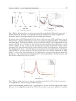
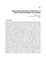
As shown in Fig.2A; the CPU reaches the maximum operational temperature after certain
time due to maximum CPU utilization. Thus the CPU utilization is reduced to the safe
utilization in order not to exceed. This phenomenon is called CPU thermal throttling. Fig.2B
shows the comparison between the ideal case “no thermal constrains”, “low power
consumption with thermal constraints” case and “high power consumption with thermal
constraints” case. The addition of more cores to the CPU chip doesn’t increase the CPU
utilization. The curve drifts to lower CPU utilization due to the CPU thermal limitation in
case of low power consumption. In case of high power consumption; the CPU utilization
decreases by adding more cores to the CPU chip. Thus the CPU utilization improvement is
not proportional to its number of cores.

Heat Transfer – Engineering Applications

380

A - thermal throttling

B- CPU Thermal throttling
Fig. 2. CPU thermal throttling (Passino & Yurkovich, 1998)
4. The advance DTM controller design
The advanced dynamic thermal management techniques are mandatory to avoid the CPU
thermal throttling. The fuzzy control provides a convenient method for constructing
nonlinear controllers via the use of heuristic information. Such heuristic information may
come from an operator who has acted as a “human-in-the-loop” controller for a process. The

fuzzy control design methodology is to write down a set of rules on how to control the
process. Then incorporate these rules into a fuzzy controller that emulates the decision-
making. Regardless of where the control knowledge comes from, the fuzzy control provides
a user-friendly and high-performance control (Patyra et al., 1996).
The DTM techniques are required in order to have maximum CPU resources utilization.
Also for portable devices the DTM doesn’t only avoid thermal throttling but also preserves
the battery consumption. The DTM controller measure the CPU cores temperatures and
according selects the speed “operating frequency” of each core. The power consumed is a
function of operating frequency and temperature. The change in temperature is a function of
temperature and the dissipated power.
The dynamic voltage and frequency scaling (DVFS) is a DTM technique that changes the
operating frequency of a core at run time (Wu et al., 2004). Clock Gating (CG)or stop-go
technique involves freezing all dynamic operations(Donald & Martonosi, 2006). CG turns
off the clock signals to freeze progress until the thermal emergency is over. When
dynamic operations are frozen, processor state including registers, branch predictor
tables, and local caches are maintained (Chaparro et al., 2007). So less dynamic power
consumed during the wait period. GC is more like suspend or sleep switch rather than an
off-switch. Thread migration (TM) also known as core hopping is a real time OS based
DTM technique. TM reduces the CPU temperature by migrating core tasks “threads” from
an overheated core to another core with lower temperature. The current traditional DTM
controller uses proportional (P controller) or proportional-integral (PI controller) or
proportional-integral-derivative (PID controller) to perform DVFS (Donald & Martonosi,
2006; Ogras et al., 2008).

Multi-Core CPU Air Cooling

381
The fuzzy logic is introduced by Lotfi A. Zadeh in 1965 (Trabelsi et al., 2004). The traditional
fuzzy set is two-dimensional (2D) with one dimension for the universe of discourse of the
variable and the other for its membership degree. This 2D fuzzy logic controller (FC) is able

to handle a non linear system without identification of the system transfer function. But this
2D fuzzy set is not able to handle a system with a spatially distributed parameter. While a
three-dimensional (3D) fuzzy set consists of a traditional fuzzy set and an extra dimension
for spatial information. Different to the traditional 2D FC, the 3D FC uses multiple sensors to
provide 3D fuzzy inputs. The 3D FC possesses the 3D information and fuses these inputs
into “spatial membership function”. The 3D rules are the same as 2D Fuzzy rules. The
number of rules is independent on the number of spatial sensors. The computation of this
3D FC is suitable for real world applications.
5. DTM evaluation index
An evaluation index for the DTM controller outputs is required. As per the thermal
throttling definition, “the operating frequency is reduced in order not to exceed the
maximum temperature”. Both frequency and temperature changes are monitored as there is
a non linear relation between the CPU frequency and temperature. One of the DTM
objectives is to minimize the frequency changes. The core theoretically should work at open
loop frequency for higher utilization. But due to the CPU thermal constrains the core
frequency is decreased depending on core hotspot temperature.
The second DTM objective is to decrease the CPU temperature as much as possible without
affecting the CPU utilization. A multi-parameters evaluation index
t

is proposed. It
consists of the summation of each parameter evaluation during normalized time period.
This index is based on the weighted sum method. The objective of multi-parameters
evaluation index shows the different parameters effect on the CPU response. Thus the
designer selects the suitable DTM controller that fulfils his requirements. The multi-
parameters evaluation index permits the selection of DTM design that provides the best
frequency parameter value without leading to the worst temperature parameter value.
The DTM evaluation index
t


calculation consists of 5 phases:
1. Identify the required parameters
2. Identify the design parameters ranges
3. Identify the desired parameters values of each range
Desired
ij


4. Identify the actual parameters values of each range
Actual
ij


5. Evaluate each parameter and the over all multi- parameter evaluation index

t

=
1
l
i
i




(1)
The parameter
i


value during the evaluation time period is the summation of the
evaluation ranges divided by the number of ranges
m
i
.

i

=
1
m
i
1
i
m
i
j
j




(2)

Heat Transfer – Engineering Applications

382
Each evaluation range
i
j


is evaluated over a normalized time period

i
j

=
Actual
ij
Desired
ij



(3)
Actual
ij

is the actual percentage of time the CPU runs at that range
Desired
ij

is the desired percentage of time the CPU runs at that range
The
i

value should be 1 or near 1. If 1
i



then the CPU runs less time than the desired
within this range. If
1
i

 then the CPU runs more time than the desired within this
range. Thus the multi-parameters evaluation index equation is:

Actual
ij
Desired
11
1
()
i
m
l
t
ij
ij
m
i







(4)

The DTM controller evaluation index desired value should be
t
l


or near l , where l is
the number of parameters. The Multi-parameters evaluation index permit the designer to
evaluate each rang independent on the other ranges and also evaluate the over all DTM
controller response.
The multi-parameters evaluation index is flexible and accepts to add more evaluation
parameters. This permits the DTM controller designer to add or remover any parameter
without changing the evaluations algorithm. Fig.3 shows an example of the parameter
i

calculation. In this example the parameter
i

is the temperature. The temperature curve is
divided into 3 ranges: High (H) – Medium (m) – Low (L), these ranges are selected as follow:
High “greater than78 °C”, Medium “between 74 °C and 78 °C”, and Low “lower than 72
°C”. The actual parameters values of each range
Actual
ij

is calculated as follow:
Actual
i Hi
g
h


=
20.5%,
Actual
i Medium

= 76%, and
Actual
i Low

=3.5%
6. Thermal spare core
As a CPU is not 100% utilized all time, thus some of the CPU cores could be reserved for
thermal crises. Consider Fig.4A, when a core reaches the steady state temperature
1
T
, the
cooling system is able to dissipate the exhausted heat outside the chip. However, if this core
is overheated, the cooling system is not able to exhaust the heat outside the chip. Thus the
core temperature increases until it reaches the thermal throttling temperature
3
T (Rao &
Vrudhula, 2007).
The same thermal phenomena, as shown in Fig.4A, occur due to faults in the cooling system
(Ferreira et al., 2007). The semiconductor technology permits more cores to be added to CPU
chip. While the total chip area overhead is up to 27.9 % as per ITRS (ITRS , 2009). That
means there is no chip area wasting in case of TSC. So reserving cores as thermal spare core
(TSC) doesn’t impact CPU over all utilization. These cores are not activated simultaneously
due to thermal limitations. According to Amdahl’s law: “parallel speedups limited by serial
portions” (Gustafson , 1988). So adding more cores to CPU chip doesn’t speedup due to the
serial portion limits. Thus not all cores are fully loaded or even some of them are not even

Multi-Core CPU Air Cooling

383

Fig. 3. Example of actual parameter value calculation
utilized if parallelism doesn't exist. The TSC concept uses the already existing chip space
due to semiconductor technology. From the thermal point of view; the horizontal heat
transfer path has for up to 30% of CPU chip heat transfer (Stan et al., 2006). The TSC is a big
coldspot within the CPU area that handles the horizontal heat transfer path. The cold TSC
reduces the static power as the TSC core is turned off. Also the TSC is used simultaneous
with other DTM technique. The equation (5) calculates number of TSCs cores. The selection
of TSC cores number is dependant on the number of cores per chip and maximum power
consumed per core as follow:

| { ( 198 ) / 198 } |
TSC mx C
NPN



(5)
where
TSC
N
: minimum number of TSCs,
mx
P
: maximum power consumed per core,
C

N
:
total number of cores, 198 Watts is the thermal limitation of the air cooling system. Fig.4A
shows core profile where lower curve is normal thermal behavior. The upper curve is the
overheated core,
1
T
is the steady state temperature,
1
T
= 80 C corresponds to the
temperature at
1
t
.
2
t
is required time for a thermal spare core to takeover threads from the
overheated core,
2
T
= 100 C corresponds to the temperature at
2
t
.
3
T
is the throttling
temperature, and
3

T
= 120 C corresponds to the temperature at
3
t
.
TSC technique uses the already existing cores within CPU chip to avoid CPU thermal
throttling as follow: Hot TSC: is a core within the CPU powered on but its clock is stopped.
It only consumes static power. It is a fast replacement core. However, it is still a heat source.
Cold TSC: is a core within the CPU chip powered off (no dynamic or static power
consumed). It is not a heat source, but it is a slow replacement core. Its activation needs
more time than hot TSC. But the cold TSC reduces the static power dissipation. Also cold
TSC generates cold spot with relative big area that helps exhausting the horizontal heat
transfer path out of the chip.

Heat Transfer – Engineering Applications

384

A- Core thermal throttling “upper” curve
(Ferreira et al., 2007).

B- The CPU congestion due to thermal
limitations

C- Activating TSC during the CPU thermal
crises

D- Activating many TSC during the CPU
thermal crises
Fig. 4. TSC Illustration

Defining
tsc
T as the TSC activation temperature as follow:

ss tsc th
TT T

(6)

min { ( ) , ( ) }
tsc thCT thTM
ttttt



(7)
Where:
ss
T
: core steady state temperature.
tsc
T
: The temperature that triggers TSC process.
th
T
: CPU throttling temperature.
tsc
t
: The time of activating TSC.
th

t
: The time required to
reach thermal throttling.
CT
t
: The estimated time required for completing the current tasks
within the over heated core. This information is not always accurate at run time.
TM
t
: Time
required migrating threads from over heated core to TSC. If any core reaches
tsc
T
then the
DTM controller will inform the OS to stop assigning new tasks to this overheated core. Thus
the OS doesn’t assign any new task to the overheated core. Therefore,
tsc
T
is not predefined
constant temperature but variable temperature between
ss
T
and
th
T
. The DTM selects
tsc
T

depending on the minimum time required to evacuate the over heated core.

6.1 TSC illustration
This section illustrates the thermal spare cores (TSC) technique
As shown in Fig.4B, the CPU is 100% utilized for duration about 50 seconds. The OS realizes
that the CPU congestion. The CPU executes its tasks slowly. In fact the CPU suffers from
thermal throttling. This CPU utilization curve shows CPU congestion from OS point of view
due to thermal limitations.
As shown in Fig.4C, The DTM controller detected the CPU high temperature. Thus the DTM
controller executes the TSC algorithm. At 40 seconds time line, a TSC core replaces a hot
core. The handover between the hot core the TSC core lead to a CPU peak. But The CPU
improves its speed after that peak; as the TSC is still cold relatively and operates at higher

Multi-Core CPU Air Cooling

385
frequency. At 86 seconds, the CPU reaches thermal throttling again. Thus the CPU reaches
congestion again. So the activation of a TSC core during the CPU thermal crises decreases
the duration of the CPU degradation from 50 seconds to 15 seconds duration.
As shown in Fig.4D, the activation of 3 TSC cores during the thermal crises at 25 seconds, 45
seconds and 85 seconds time lines respectively increases the CPU utilization. The CPU
executes its tasks normally without congestion rather than some CPU peaks. AS this CPU
chip has many spare cores; the DTM controller activates the required TSC during the CPU
thermal crises. So the CPU avoids the thermal throttling theoretically.
6.2 3D Fuzzy DTM controller
The 3D fuzzy control is able to handle the correlation between the different variable
parameters of a distributed parameter system (Li & Li, 2007). Thus the 3D fuzzy logic is able
to process the Multi-Core CPU correlation information. The 3D fuzzy control demonstrates
its potential to a wide range of engineering applications. The 3D fuzzy control is feasible for
real-time world applications (Li & Li, 2007). The thermal management process is a
distributed parameter systems. The thermal management process is represented by the
nonlinear partial differential equations (Doumanidis & Fourligkas, 2001).

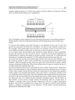
Fig. 5. Actuator
u and the measurement sensors at
p
point.
Fig.5. presents a nonlinear distributed parameter system with one actuator (
1

 ). Where
p
point measurement sensors are located at
12
, , ,
p
zz z in the one-dimensional space
domain respectively and an actuator
u with some distribution acts on the distributed
process. Inputs are measurement information from sensors at different spatial
locations. i.e., deviations
12
, , ,
p
ee e and deviations change
12
, , ,
p
ee e

 where

1
() (,)
di i
eyzyzn
,
() ( 1)
ii i
eenen



()
di
y
z
denotes the measurement value
from location
i
z
, , 1nn

denote the n and 1n

sample time input. The output relationship
is described by fuzzy rules extracted from knowledge. Since
p
sensors are used to provide
2
p
inputs.

Fig. 6. 3D fuzzy set (Li & Li, 2007)

Heat Transfer – Engineering Applications

386
The 3D fuzzy control system is able to capture and process the spatial domain information
defined as the 3D FC. One of the essential elements of this type of fuzzy system is the 3D fuzzy
set used for modeling the 3D uncertainty. A 3D fuzzy set is introduced in Fig.6 by developing
a third dimension for spatial information from the traditional fuzzy set. The 3D fuzzy set
defined on the universe of discourse
X and on the one-dimensional space is given by:

{(,), (,) , }
V
Vxz xz xXzZ

and 0 {(,), (,) 1
V
xz xz




(8)
When
X
and
Z

are discrete, V is commonly written as (,)/(,)
V
zZ xX
Vxzxz






Where

denotes union over all admissible x and z . Using this 3D fuzzy set, a 3D
fuzzy membership function (3D MSF) is developed to describe a relationship between input
x and the spatial variable z with the fuzzy grade u .


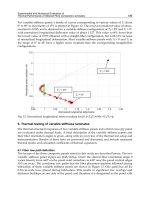
A - 3D fuzzy system block diagram

B- Spatial information fusion at each crisp input
z
x
Fig. 7. 3D fuzzy system illustration (Li & Li, 2007)
Theoretically, the 3D fuzzy set or 3D global fuzzy MSF is the assembly of 2D traditional
fuzzy sets at every spatial location (Li & Li, 2007). However, the complexity of this global 3D

Multi-Core CPU Air Cooling

387
nature may cause difficulty in developing the FC. Practically, this 3D fuzzy MSF is

approximately constructed by 2D fuzzy MSF at each sensing location. Thus, a centralized
rule based is more appropriate, which avoid the exponential explosion of rules when
sensors increase. The new FC has the same basic structure as the traditional one. The 3D FC
is composed of fuzzification, rule inference and defuzzification as shown in Fig.7A. Due to
its unique 3D nature, some detailed operations of this new FC are different from the
traditional one. Crisp inputs from the space domain are first transformed into one 3D fuzzy
input via the 3D global fuzzy MSF. This 3D fuzzy input goes through the spatial information
fusion and dimension reduction to become a traditional 2D fuzzy input. After that, a
traditional fuzzy inference is carried out with a crisp output produced from the traditional
defuzzification operation. Similar to the traditional 2D FC, there are two different
fuzzifications: singleton fuzzifier and non-singleton.
A singleton fuzzifier is selected as follows: Let
A be a 3D fuzzy set,
x
is a crisp input,
xX and z is a point zZ

in one-dimensional space
Z
. The singleton fuzzifier maps
x
into A in X at location
z
then A s a fuzzy singleton with support 'x if (,) 1
A
xz

 for
'
xx , 'zz and (,) 0

A
xz


for all other xX

, zZ

with 'xx

, 'zz

if finite sensors
are used. This 3D fuzzification is considered as the assembly of the traditional 2D
fuzzification at each sensing location. Therefore, for
p
discrete measurement sensors located
at
12
, , ,
p
zz z
,
12
[ ( ), ( ), , ( )]
zj
xxzxzxz

is defined as J crisp spatial input variables in
space domain

12
{ , , , }
p
Zzz z

where ( ) ( 1,2, , )
ji j
xz X IR
j
J

 denotes the crisp input
at the measurement location
i
zz

for the spatial input variable
()
j
xz
,
j
X
denotes the
domain of ( )
j
i
xz. The variable ( )
j
xzis marked by “

z
” to distinguish from the ordinary
input variable, indicating that it is a spatial input variable. The fuzzification for each crisp
spatial input variable ( )
j
xzis uniformly expressed as one 3D fuzzy input
x
j
A
in the discrete
form as follows:
11
1111
()
( ( ), )/( ( ), )
XX
zZ x z X
Axzzxzz






()
((),)/((),)
JJ
XJ XJ J J
zZ x z X
Axzzxzz







Then, the fuzzification result of J crisp inputs
z
x can be represented by:

X
A =
1122
11
() () ()
{ ( ( ), ) * * ( ( ), )} /
JJ
XXJJ
zZ x z X x z X x z X
xzz xzz

 
  


1
{( ( ), ) * *( ( ), )}
J
xzz xzz

(9)
Where * denotes the triangular norm; t-norm (for short) is a binary operation. The t-norm
operation is equivalent to logical AND. Also it has been assumed that the membership
function
X
A

is separable .
Using the 3D fuzzy set, the
th

rule in the rule based is expressed as follows:

Heat Transfer – Engineering Applications

388

1
1
: ( ) ( )
JJ
RifxzisCand andxzisCthenuisG




(10)
Where
R


denotes the
th

rule (1, 2, , )N


( ),( 1,2, , )
j
xz
j
J

denotes spatial input variable
J
C

denotes 3D fuzzy set, u denotes the control action uUIR

 ,G

denotes a
traditional fuzzy set N is the number of fuzzy rules, the inference engine of the 3D FC is
expected to transform a 3D fuzzy input into a traditional fuzzy output. Thus, the inference
engine has the ability to cope with spatial information. The 3D fuzzy DTM controller is
designed to have three operations: spatial information fusion, dimension reduction,
and traditional inference operation. The inference process is about the operation of
3D fuzzy set including union, intersection and complement operation. Considering the
fuzzy rule expressed as (10), the rule presents a fuzzy relation
1
:

J
RC C G


  (1, 2, , )N

 thus, a traditional fuzzy set is generated via
combining the 3D fuzzy input and the fuzzy relation is represented by rules.
The spatial information fusion is this first operation in the inference to transform the 3D
fuzzy input
X
A into a 3D set W

appearing as a 2D fuzzy spatial distribution at each
input
z
x . W

is defined by an extended sup-star composition on the input set and
antecedent set. Fig.7B. gives a demonstration of spatial information fusion in the case of two
crisp inputs from the space domain
Z ,
12
[ ( ), ( ), , ( )]
zj
xxzxzxz

.
This spatial 3D MSF, is produced by the extended sup-star operation on two input sets from
singleton fuzzification and two antecedent sets in a discrete space

Z at each input value
z
x .
An extended sup-star composition employed on the input set and antecedent sets of the
rule, is denoted by:

1
( )
( )
1
o
o
J
X
Ax
CC
WA
CC
J








(11)
The grade of the 3D MSF derived as

( )
1
() ( ,)
z
o
W
A
XC C
J
zxz







(12)
11
1
( ) , , ( )
() sup [ ( ,)* ( ,)]
JJ
J
xzX xzX z z
AX
W
CC
zxzxz






 where zZ

and * denotes the
t-norm operation.
11
1
( ) , , ( ) 1
1
1
() sup [ ( (),)*
* ( ( ), ) * ( ( ), ) *
JJ
xzX xzX
AX
W
J
AXJ
C
zxzz
xzz xzz







1
1
* ( ( ), ) * * ( ( ), )]
J
J
CC
xzz xzz




11
1
() 1 1
1
()
( ) {sup [ ( ( ), ) ( ( ), )]} *
* {sup [ ( ( ), ) ( ( ), )]}
JJ
J
xzX
AX
W
C
xzX J J
AXJ
C
zxzzxzz
xzz xzz










The dimension reduction operation is to compress the spatial distribution information
(,,)
z
xz

into 2D information (,)
z
x

as shown in Fig.7B. The set W

shows an approximate

Multi-Core CPU Air Cooling

389
fuzzy spatial distribution for each input
z
x in which contains the physical information. The
3D set
W


is simply regarded as a 2D spatial MSF on the plane (,)z

for each input
z
x .
Thus, the option to compress this 3D set
W

into a 2D set


is approximately described as
the overall impact of the spatial distribution with respect to the input
z
x
.The traditional
inference operation is the last operation in the inference. Where implication and rules’
combination are similar to those in the traditional inference engine.

() * (),
VG
uuuU






(13)
Where * stands for a t-norm, ( )

G
u


is the membership grade of the consequent set of the
fired rule
R

. Finally, the inference engine combines all the fired rules (14) .Where V

the
output is fuzzy set of the fired rule
R

,'N denotes the number of fired rules and V denotes
the composite output fuzzy set.

'
1
N
VV






(14)
The traditional defuzzification is used to produce a crisp output. The center of area (COA) is
chosen as the defuzzifier due to its simple computation (Yager et al., 1994).

'
1
'
1
N
N
C
u















(15)
Where
CU

 is the centroid of the consequent set of the fired rule
R


(1, 2, , ')N

 which
represents the consequent set
G

in (13), 'N is the number of fire rules 'NN


For Multi-Core CPU system; each core is considered as heat source. The heat conduction
Q path is inverse propositional to the distance between the heat sources (16). The nearest
hotspot has the highest effect on core temperature increase. Also the far hotspot has the
lowest effect on core temperature increase.

AT
Q
d




(16)
Where Q is the heat conducted,

the thermal conductivity,
A
the cross-section area of
heat path (constant value),
T


the temperature difference at the hotspots locations, d the
length of heat path (the distance between the heat sources). The 3D MSF gain
i
j
G is selected
as the inverse the distance between 2 cores hotspots locations

32DDij
MSF MSF G


(17)
Where
2D
M
SF the 2D MSF,
i
j
G the correlation gains between core i and core j.
i
j
G is not a
constant value as the hotspots locations are changing during the run time. The maximum
gain = 1 in case of calculating the correlation gain locally
ii
G .

Heat Transfer – Engineering Applications

390
The 3D FC is based on 32 variables as follow (Yager et al., 1994):
The inputs 3D fuzzy variable at step n for each core are: 8 frequency deviation variables
calculate as per (3). The output: for each core, the output is the core operating frequency at
step n+1. The relationships: at step n CPU throughput is proportional to cores operating
frequency. The core operating frequency is also proportional to the power consumption. The
maximum power consumption leads to the maximum temperature increase.
In order to compare between the 2D FC and the 3D FC responses, the same configuration
are reused with the 3D FC. The same the control objectives. The same fuzzy inputs, the same
Meta decisions rules, the same rule space , and the same input 2D MSF Normal distribution
configurations. Also The output membership functions are tuned per DTM controller. In
general we have four outputs MSF: Max - DVFS - TSC MSF - FS. Thus the only design
different between the 2D FC and the 3D FC that the 3D FC DTM takes into consideration the
surrounding core hotspot temperatures and their operating frequencies. Fig.8. shows the 3D
fuzzy DTM controller implementation.
3D-Fuzzy Example:
The number of
p
sensors = 5; the sensors are located at
12 5
, , ,zz z Two crisp input,
xX and z is a point zZ

in one-dimensional space . For 5p

discrete measurement
sensors located at
12 5
, , ,zz z
,

12
[(),()]
z
xxzxz
is defined as J is two crisp spatial input
variables in space domain
12 5
{ , , , }Zzz z

where
() ( 1,2)
ji j
xz X IRj


. The
fuzzification for each crisp spatial input variable ( )
j
xzis uniformly expressed as the 3D
fuzzy inputs are
1x
A
and
2x
A
in the discrete form. As shown in Fig.7B;
1

values are the
local substitutions of

1
()xz in each 2D MSF at each z location.
2

values are the local
substitutions of
2
()xzin each 2D MSF at each z location.
1
W

values are the sup-star
composition of
1

and
2

at each z location as shown in Table 1. The sup-star composition
in the fuzzy inference engine becomes a sup- minimum composition.

1
()xz

2
()xz

z
1


2


1
W


- 0.5 - 0.6 0.0 0.8 0.4 0.4
0.0 0.2 0.5 0.8 0.9 0.8
0.3 0.1 0.25 0.9 1 0.9
0.7 0 0.75 0.6 0.7 0.6
0.2 -0.1 1 0.8 0.3 0.3
Table 1. 3D Fuzzy with Two crisp input example
7. Simulation results
Simulation is used for validating the designed 3D fuzzy DTM controller. The CPU chip
selection is based on the on the amount of published information. The IBM POWER
processor family is selected based on published information include floor plan, thermal
design power (TDP), technology, chip area, and operating frequencies. IBM POWER4 MCM
chip is selected chip. The floor plans of the POWER4 processor and the MCM are published

Multi-Core CPU Air Cooling

391
e
f
e
f

e

T
e
T

e
f
e
f

e
T
e
T


Fig. 8. 3D-Fuzzy controller block diagram

Heat Transfer – Engineering Applications

392
as pictures. The entire processor manufacturers consider the CPU floor plan and its power
density map as confidential data. Thus there is major difficulty to build a thermal model
based on real CPU chip information. Only old CPU chip thermal data is published. The
MCM POWER4 floor plan and power density map are published. The only way to build up
a CPU thermal model is the reverse engineering of IBM MCM POWER4 chip Fig.9. The
reverse engineering process took a lot of time and efforts. The extracted MCM POWER4
chip is scaled into 45nm technology as POWER4 chip is built on the old 90nm technology
(Sinharoy et al., 2005).

Fig. 9. The extracted IBM POWER4 MCM floor plan
Virginia Hotspot simulator is selected based on simulator features and on line support
provided by Hotspot team at Virginia University. The Hotspot 5 simulator uses the duality
between RC circuits and thermal systems to model heat transfer in silicon. The Hotspot 5
simulator uses a Runge-Kutta (4th order) numerical approximation to solve the differential
equations that govern the thermal RC circuit’s operation (LAVA , 2009).
7.1 Simulation analysis
All simulations starts from 814 seconds as the CPU thermal model required 814 seconds to
reach
Control
T 70 °C. Assuming that the CPU output response follows the open loop curve
until it reaches 70 °C. At
Control
T
, the DTM controller output selects the cores operating
frequency. Then each core temperature changes according to its operating frequency. All
DTM fuzzy designs tuning are based on their output membership functions (MSF) tuning
without changing the fuzzy rules. The DTM evaluation index covers the simulation times
between 814 seconds to 1014 seconds. Theses simulation tests 3D-FC1, FC1, 3D-FC2, FC2,
3D-FC3 and FC3 perform both DVFS and TSC together. But these tests FC4, 3D-FC4, 3D-

Multi-Core CPU Air Cooling

393
FC5, and 3D-FC6 perform DVFS only. The DTM controller evaluation index (4) has only two
parameters
2l , the frequency and the temperature. Its desired value is 2
t

 or near 2.

There are two DTM evaluation index implementations presented in this section. The first
DTM implementation assumed that the CPU is required to run 20% of its time at the
maximum frequency, 50% of its time at high frequency, 20% of its time at medium
frequency and 10% of it is time at low frequency. Also the CPU is required to 30% of its time
at high temperature, 40% at medium temperature, and 30% of its time at low temperature.
This first DTM requirement evaluation against the DTM controller designs are as follow:
Table 2 shows the percentage of time when the CPU operates at each frequency ranges.
Table 3 shows the percentage of time of the CPU operates at each temperature ranges. The
best results are highlighted in bold. The DTM evaluation index selected FC3 and 3D-FC6 as
the best DTM controller designs as shown in Table 4. The best results are highlighted in
bold. Only FC3 and 3D-FC6 controllers have high results in both frequency, and
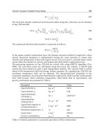
temperature evaluation indexes. As shown in Fig.10A, both DTM controllers’ frequency
change responses oscillate all times. The 3D-FC6 controller has less number of frequency
oscillation and smaller amplitudes. The FC3 controller operates at maximum frequency then
it is switched off between 1014 and 1100 seconds. The 3D-FC6 controller is never switched
off and operates at high frequency ranges but not on the maximum frequency. From the
temperature point of view; both controllers temperatures are oscillating. 3D-FC6 controller
has minimum temperature amplitudes at 970 and 1070 seconds as shown in Fig.10B. The
3D-FC6 is always operating on lower temperature than the FC3 controller. Thus the 3D-FC6
controller is better then the FC3 controller. As shown in Table 5, Table 6, Table 7; only FC4,
3D-FC3 and 3D-FC6 controllers have high results in both frequency, and temperature
evaluation indexes. As shown in Fig.10 A,C,E, all DTM controllers’ frequency change
responses oscillate all times. The 3D-FC6 controller has the lowest number of frequency
oscillation. The 3D-FC3 controller has smallest frequency changes amplitudes. The 3D-FC3
controller operates at high frequency ranges but not on the maximum frequency. From the
temperature point of view; all controller temperature are increasing as shown in Fig.10
B,D,F. The 3D-FC6 temperature is oscillating and has minimum temperature amplitudes at
970 and 1070 seconds. There is no large advantage of any controllers over the others from
temperature point of view. Thus the 3D-FC3 is better then the FC4 controller, and the 3D-
FC6 controller as the 3D-FC3 controller operates at higher frequency ranges and almost the

same temperature ranges.
Some observations are extracted from these two DTM evaluation index implementations as
follow: 3D-FC5 vs. 3D-FC6: In the first implementation the DTM evaluation index of both
controllers are almost the same from the frequency point of view. The standard deviation of
the DVFS membership function (MSF) is the same but the mean is shifted by 0.2. This shift
leads to insignificant frequency objective change but also leads to less CPU temperature. In
the second implementation the DTM evaluation index values are totally different. So the
similarity between any 2 DTM controller responses for a specific DTM design objective is
not maintain for other DTM design objective. 2D Fuzzy vs. 3D Fuzzy: These DTM
controllers share the same input and output membership functions. The correlation between
the CPU cores has significant effect i.e. (FC1 vs. 3D-FC1) and (FC3 vs. 3D-FC3). But for (FC2
vs. 3D-FC2) there is almost no correlation effect in both DTM evaluation index
implementations. This means that the selection of non proper membership functions could
ignore the correlation effect between the CPU cores. (TSC+DVFS) vs. (DVFS alone): the

Heat Transfer – Engineering Applications

394
DTM temperature design objectives could be fulfilled by TSC+DVFS or by DVFS alone i.e.
3D-FC3 vs. 3D-FC4. The driver for using TSC with DVFS is the CPU thermal throttling
limits. So if DVFS can fulfil alone the temperature DTM design objective then there is no
need for combining both TSC with DVFS.


Frequecny Change
0
10
20
30
40

50
60
70
80
90
100
860 910 960 1010 1060 1110
Time in seconds
Frequency Change
FC3
3D-FC6

A - frequency comparisons of FC3 and 3D-FC6

Response
72
74
76
78
80
82
84
86
88
860 960 1060
Time in Seconds
Max HotSpot Temperature in C
open loop
FC3
Threshold

3D-FC6

B- temperature comparisons of FC3 and
3D-FC6
Frequecny Change
0
10
20
30
40
50
60
70
80
90
100
860 910 960 1010 1060 1110
Time in seconds
Frequency Change
3D-FC3
FC4

C- frequency comparisons of FC4 and 3D-FC3

Response
72
74
76
78
80

82
84
86
88
860 960 1060
Time in Seconds
Max HotSpot Temperature in C
open loop
3D-FC3
Threshold
FC4

D- temperature comparisons of FC4 and
3D-FC3

Frequecny Change
0
10
20
30
40
50
60
70
80
90
100
860 910 960 1010 1060 1110
Time in seconds
Frequency Change

3D-FC5
3D-FC6

E -frequency comparisons of 3-FC5 and
3D-FC6
Response
72
74
76
78
80
82
84
86
88
860 960 1060
Time in Seconds
Max HotSpot Temperature in C
open loop
Threshold
3D-FC5
3D-FC6

F- temperature comparisons of 3D-FC5
and 3D-FC6
Fig. 10. The Simulation Results

Multi-Core CPU Air Cooling

395

Controller
Name
Frequency Ranges %
Actual
1j


Frequency Ranges
Values
1
j


1


(M)
j=1
(H)
j=2
(m)
j=3
(L)
j=4
(M)
j=1
(H)
j=2
(m)

j=3
(L)
j=4
Desired
1j


20% 50% 20% 10% 1.0 1.0 1.0 1.0 1.00
Switch 0% 100% 0% 0% 0 2 0% 0 0.500
P 10% 0% 22% 22% 2.7 0.0 1 2 1.528
FC1 12% 22% 44% 22% 0.5 0.4 2 2.2 1.315
3D-FC1 0% 10% 33% 11% 0.0 1.1 1.7 1.1 0.972
FC2 0% 100% 0% 0% 0.0 2.0 0.0 0.0 0.500
3D-FC2 0% 89% 11% 0% 0.0 1.8 0.6 0.0 0.123
FC3 22% 22% 10% 0% 1.1 0.4 2.8 0.0 1.083
3D-FC3 0% 78% 22% 0% 0.0 1.6 1.1 0.0 0.667
FC4 0% 66% 33% 0% 0.0 1.3 1.7 0.0 0.750
3D-FC4 22% 10% 22% 0% 1.1 1.1 1.1 0.0 0.833
3D-FC5 0% 10% 33% 11% 0.0 1.1 1.7 1.1 0.972
3D-FC6 0% 78% 0% 22% 0.0 1.6 0.0 2.2 0.944
Table 2. The frequency comparisons of the first implementation

Controller
Name
Temperature Ranges %
Actual
2j


Temperature

Ranges
Values

2
j


2


(H)
j=1
(m)
j=2
(L)
j=3
(H)
j=1
(m)
j=2
(L)
j=3
Desired
2 j


30% 40% 30% 1.0 1.0 1.0 1.00
Switch 0.0% 100% 0.0% 0.0 2.5 0.0 0.83
P 78% 0% 22% 2.6 0.0 0.7 1.11
FC1 11% 89% 0% 0.4 2.2 0.0 0.86

3D-FC1 22% 78% 0% 0.7 1.9 0.0 0.90
FC2 67% 33% 0% 2.2 0.8 0.0 1.02
3D-FC2 10% 44% 0% 1.8 1.1 0.0 0.99
FC3 67% 33% 0% 2.2 0.8 0.0 1.02
3D-FC3 33% 67% 0% 1.1 1.7 0.0 0.93
FC4 44% 10% 0% 1.5 1.4 0.0 0.96
3D-FC4 33% 67% 0% 1.1 1.7 0.0 0.93
3D-FC5 0% 100% 0% 0.0 2.5 0.0 0.83
3D-FC6 33% 10% 11% 1.1 1.4 0.4 0.96
Table 3. The temperature comparisons of the first implementation

Heat Transfer – Engineering Applications

396


Controller
Name
Frequency
Index
1


Temperature
Index
2


The Evaluation
Index

t


Desired
1.00 1.00 2.00
Switch
0.500 0.83 1.33
P
1.528 1.11 2.64
FC1
1.315 0.86 2.23
3D-FC1
0.972 0.90 1.87
FC2
0.500 1.02 1.52
3D-FC2
0.123 0.99 1.11
FC3
1.083 1.02 2.10
3D-FC3
0.667 0.93 1.13
FC4
0.750 0.96 1.71
3D-FC4
0.833 0.93 1.76
3D-FC5
0.972 0.83 1.81
3D-FC6
0.944 0.96 1.90

Table 4. The DTM evaluation index of the first implementation


Controller
Name
Frequency Ranges %
Actual
1j


Frequency Ranges
Values

1
j


1


(M)
j=1
(H)
j=2
(m)
j=3
(L)
j=4
(M)
j=1

(H)
j=2
(m)
j=3
(L)
j=4
Desired
1j


10% 70% 10% 10% 1.0 1.0 1.0 1.0 1.00
Switch 0% 100% 0% 0% 0.0 1.4 0.0 0.0 0.311
P 10% 0% 22% 22% 5.6 0.0 2.2 2.2 2.500
FC1 12 22% 44% 22% 1.1 0.3 4.4 2.2 2.024
3D-FC1 0% 10% 33% 11% 0.0 0.8 3.3 1.1 1.309
FC2 0% 100% 0% 0% 0.0 1.4 0.0 0.0 0.311
3D-FC2 0% 89% 11% 0% 0.0 1.3 1.1 0.0 0.135
FC3 22% 22% 10% 0% 2.2 0.3 5.6 0.0 2.024
3D-FC3 0% 78% 22% 0% 0.0 1.1 2.2 0.0 0.833
FC4 0% 67% 33% 0% 0.0 0.9 3.3 0.0 1.071
3D-FC4 22% 10% 22% 0% 2.2 0.8 2.2 0.0 1.309
3D-FC5 0% 10% 33% 11% 0.0 0.8 3.3 1.1 1.309
3D-FC6 0% 78% 0% 22% 0.0 1.1 0.0 2.2 0.833

Table 5. The frequency comparisons of the second implementation

Multi-Core CPU Air Cooling

397
Controller Name

Temperature Ranges %
Actual
2j


Temperature
Ranges
Values

2
j


2


(H)
j=1
(m)
j=2
(L)
j=3
(H)
j=1
(m)
j=2
(L)
j=3
Desired
2 j



30% 40% 30% 1.0 1.0 1.0 1.00
Switch 0% 100% 0% 0.0 2.0 0.0 0.67
P 78% 0% 22% 3.9 0.0 0.7 1.54
FC1 111% 89% 0% 0.6 1.8 0.0 0.78
3D-FC1 22% 78% 0% 1.1 1.6 0.0 0.89
FC2 67% 33% 0% 3.3 0.7 0.0 1.33
3D-FC2 10% 44% 0% 2.8 0.9 0.0 1.22
FC3 67% 33% 0% 3.3 0.7 0.0 1.33
3D-FC3 33% 67% 0% 1.7 1.3 0.0 1.00
FC4 44% 10% 0% 2.2 1.1 0.0 1.11
3D-FC4 33% 67% 0% 1.7 1.3 0.0 1.00
3D-FC5 0% 100% 0% 0.0 2.0 0.0 0.67
3D-FC6 33% 10% 11% 1.7 1.1 0.4 1.05
Table 6. The temperature comparisons of the second implementation

Controller
Name
Frequency
Index
1


Temperature
Index
2


The Evaluation

Index
t


Desired 1.00 1.00 2.00
Switch 0.311 0.67 1.02
P 2.500 1.54 4.04
FC1 2.024 0.78 2.80
3D-FC1 1.309 0.89 2.20
FC2 0.311 1.33 1.69
3D-FC2 0.135 1.22 1.82
FC3 2.024 1.33 3.36
3D-FC3
0.833 1.00 1.83
FC4
1.071 1.11 2.18
3D-FC4
1.309 1.00 2.31
3D-FC5
1.309 0.67 1.98
3D-FC6
0.833 1.05 1.88
Table 7. The DTM evaluation index of the second implementation
8. Conclusion
Moore’s Law continues with technology scaling, improving transistor performance to
increase frequency, increasing transistor integration capacity to realize complex

Heat Transfer – Engineering Applications

398

architectures, and reducing energy consumed per logic operation to keep power dissipation
within limit. The technology provides integration capacity of billions of transistors;
however, with several fundamental barriers. The power consumption, the energy level,
energy delay, power density, and floor planning are design challenges. The Multi-Core CPU
design increases the CPU performance and maintains the power dissipation level for the
same chip area. The CPU cores are not fully utilized if parallelism doesn't exist. Low cost
portable cooling techniques exploration has more importance everyday as air cooling
reaches its limits “198 Watt”. In order to study the Multi-Core CPU thermal problem a
thermal model is built. The thermal model floor plan is similar to the IBM MCM POWER4
chip scaled to 45nm technology. This floor plan is integrated to the Hotspot 5 thermal
simulator. The CPU open loop thermal profile curve is extracted. The advanced dynamic
thermal management (DTM) techniques are mandatory to avoid the CPU thermal throttling.
As the CPU is not 100% utilized all time, the thermal spare cores (TSC) technique is
proposed. The TSC technique is based on the reservation of cores during low CPU
utilization. These cores are not activate simultaneously due to limitations. During thermal
crises, these reserved cores are activated to enhance the CPU utilization. The semiconductor
technology permits more cores to be added to CPU chip. But the total chip area overhead is
up to 27.9 % as per ITRS (ITRS , 2009). That means there is no chip area wasting in case of
TSC. From the thermal point of view; the horizontal heat transfer path has up to 30% of CPU
chip heat transfer (Stan et al., 2006). The TSC is a big coldspot within the CPU area that
handles the horizontal heat transfer path.
The cold TSC also handles the static power as the TSC core is turned off. The TSC is used
simultaneous with other DTM technique. From the CPU utilization point of view, the TSC
activation is equivalent to the CPU cores DVFS for a low operating frequency range. Fuzzy
logic improves the DTM controller response. Fuzzy control handles the CPU thermal
process without knowing its transfer function. This simplifies the DTM controller design
and reduces design time. The fuzzy control permits the designers to select the appropriate
CPU temperature and frequency responses. For the same CPU chip, the DTM response
depends on the DTM fuzzy controller design. As the 3D fuzzy permits the preservation of
portable device battery but this affects the CPU utilization. Or it permits the high

performance computing (HPC). But due to cooling limitation this DTM design is not
suitable for the portable devices. The 3D-FC is successfully implemented to the CPU DTM
problem. Different DTM techniques are compared using simulation tests. The results
demonstrate the effectiveness of the 3D fuzzy DTM controller to the nonlinear Multi-Core
CPU thermal problem. The 3D fuzzy DTM takes into consideration the surrounding core
hotspot temperatures and operating frequencies. The 3D fuzzy DTM avoids the complexity
and maintains the correlations. As the 3D fuzzy DTM controller calculates the correlation
between local core hotspot and the surrounding cores hotspots. Then it selects the
appropriate local core operating frequency. The Fuzzy DTM controller has better response
than the traditional DTM P controller. For the same input rules and the same output
membership functions (MSF), the 3D fuzzy logic reduces the CPU temperature better than
the 2D fuzzy logic. The fuzzy output MSF is a critical DTM design parameter. The small
deviation from the appropriate output membership function affects the DTM controller
behavior.
The Fuzzy DTM controller has better response than the traditional DTM P controller. For the
same input rules and the same output membership functions (MSF), the 3D Fuzzy logic

Multi-Core CPU Air Cooling

399
reduces the CPU temperature better than the 2D Fuzzy logic. The 3D Fuzzy controller takes
into consideration multiple temperatures readings distributed over the CPU chip floor plan.
The Fuzzy control permits the designers to select the appropriate CPU temperature and
frequency responses. For the same CPU chip, the DTM response depends on the Fuzzy
controller design. The fuzzy output MSF is a critical DTM design parameter. The small
deviation from the appropriate output membership function affects the DTM controller
behavior. From the CPU temperature point of view; the TSC looks like a large coldspot. The
cold TSC absorb the horizontal heat path as if it is a heatsink pipe. The CPU cooling system
behavior depends on the combinations of the operating frequencies and temperatures. The
objective of multi-parameters evaluation index is to show the different parameters effect on

the CPU response. Thus the designer selects the suitable DTM controller that fulfils his
requirements. The multi-parameters evaluation index permits the selection of DTM design
that provides the best frequency parameter value without leading to the worst temperature
parameter value.
9. References
Chaparro, P. ; Lez, J. G. Cai, Q. & Lez, A. G. (2007). Understanding The Thermal
Implications of Multicore Architectures, IEEE Transactions, Vol.18, No.8, pp. 109-
1065.
Chung, S. W. ; & Skadron, K. (2006). Using on-chip event counters for high-resolution, real-
time temperature measurements, Proceedings of International Conference For
Scientific & Engineering Exploration Of Thermal, Thermomechanical & Emerging
Technology, IEEE ITHERM06, pp. 114-120.
Donald, J. ; & Martonosi, M. (2006). Techniques For Multicore Thermal Management
Classification & New Exploration, Proceedings of International Symposium on
Computer Architecture, IEEE ISCA’06, pp. 78-88.
Doumanidis, C. C.; & Fourligkas, N. (2001). Temperature Distribution Control In Scanned
Thermal Processing Of Thin Circular Parts, IEEE Transaction Control System
Technolgy, Vol.9, No.5, (May 2001), pp. 708–717.
Ferreira, A. P.; Moss,D. & Oh, J. C. (2007). Thermal Faults Modeling using an RC model with
an Application to Web Farms, Proceedings of 19th Euromicro Conference on Real-
Time Systems,Italy, pp. 113-124.
Huangy, W. ; Stany, M. R. Skadronz,K. Sankaranarayananz, K. Ghoshyz, S. & VelUSAmyz, S
(2006). Hotspot: A Compact Thermal Modeling Methodology For Early-Stage Vlsi
Design, IEEE Transactions, 2006, Vol.5, pp. 501-513.
Gustafson, J. L.(1988). Re-Evaluating Amdahl’s Law, ACM Communications, Vol.31, No.5,
pp. 82-83.
Kim, D. D.; J. Kim, Cho, C. Plouchart, J.O. & Trzcinski, R. (2008). 65nm SOI CMOS SoC
Technology for Low-Power mmWave & RF Platform, Silicon Monolithic Integrated
Circuits in RF Systems, pp. 46-49.
Kim, S. ; Dick, R. P. & Joseph, R. (2007). Power Deregulation: Eliminating Off-Chip Voltage

Regulation Circuitry From Embedded Systems, Proceedings of the International
Conference on Hardware-Software Codesign & System Synthesis, IEEE/ACM
(CODES+ISSS), pp. 105-110.

Heat Transfer – Engineering Applications

400
Li, H. Zhang; X. & Li, S. (2007). A Three-Dimensional Fuzzy Control Methodology For A
Class Of Distributed Parameter Systems, IEEE Transactions, Fuzzy Systems, Vol.15,
No.3, pp. 470-481.
Mccrorie, P. (2008). On-Chip Thermal Analysis Is Becoming M&atory, Chip Design Magazine.
Moore, G. E. (1965). Cramming More Components Onto Integrated Circuits, IEEE
Electronics,Vol.38, No.8, (19 April 1965), pp.114. This Paper Appears Again In IEEE
Solid-State Circuits Newsletter, 2006, Vol.20, No.3, pp. 33-35.
Ogras, U.Y. et al. (2008). Variation-Adaptive Feedback Control for Networks-on-Chip with
Multiple Clock Domains, Proceedings of International Conference on Design
Automation Conference, IEEE DAC08, pp. 154-159.
Passino, K. M.; & Yurkovich, S. (1998). Fuzzy Control, Addison Wesley Longman.
Patyra, M. J.; Grantner, J.L. & Koster, K. (1996). Digital Fuzzy Logic Controller Design &
Implementation, IEEE Transactions Fuzzy Systems, Vol.4, No.4, pp. 439-413.
Rao, R. ; & Vrudhula, S. (2007). Performance Optimal Processor Throttling Under Thermal
Constraints, Proceedings of International Conference On Compilers, Architecture, &
Synthesis For Embedded Systems, CASES’07, pp. 211-266.
Sinharoy, B.; Kalla, R. N. Tendler, J. M. & Eickemeyer,R. J. (2005). POWER5 System
Microarchitecture, IBM J. Res. & Dev. Vol.49 No. 4/5 July/September 2005.
Stan, M. R. ; Skadron, K. Barcella, M. Sankaranarayanan, W. H. K. & Velusamy, S. (2006).
Hotspot: A Compact Thermal Modeling Methodology For Early-Stage VLSI Design,
IEEE Transactions, Vol.14, No.5, pp. 501-513.
Trabelsi, A. ; Lafont, F. Kamoun, M. & Enea, G. (2004). Identification of Nonlinear
Multivariable Systems By Adaptive Fuzzy Takagi-Sugeno Model, International

Journal of Computational Cognition, Vol.2, No.3, pp. 137-18.
Wu, Q. et al. (2004). Formal online methods for voltage/frequency control in multiple clock
domain microprocessors, Proceedings of International Conference on Architectural
Support for Programming Languages and Operating Systems, ASPLOS, Vol.32, No.5,
pp. 248-213.
Yager, R. ; & Filev, D. (1994). Essential Of Fuzzy Modeling & Control, Wiley, New York 1994,
pp. 121.