Thermodynamics Kinetics of Dynamic Systems Part 4 pdf

Modeling and Simulation for Steady State and Transient Pipe Flow of Condensate Gas

79


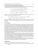
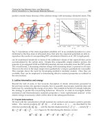
Fig. 9. The steady state liquid velocity variations of the condensate gas pipeline





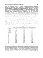
Fig. 10. The steady state liquid holdup variations of the condensate gas pipeline
The feature of condensate gas pipelines is phase change may occur during operating. This
leads to a lot of new phenomena as follow:
1.
It can be seen from Fig.6 that the pressure drop curve of two phase flow is significantly
different from of gas flow even the liquid holdup is quite low. The pressure drop of gas
flow is non-linear while the appearance of liquid causes a nearly linear curve of the
pressure drop. This phenomenon is expressed that the relatively low pressure in the
pipeline tends to increase of the gas volume flow; the appearance of condensate liquid
and the temperature drop reduce the gas volume flow.
2.
It can be seen from Fig. 7 that the temperature drop curve of two phase flow is similar
to single phase flow. The temperature drop gradient of the first half is greater than the
last half because of larger temperature difference between the fluid and ambient.

Thermodynamics – Kinetics of Dynamic Systems

80
3. It can be seen from Fig. 8 and Fig.9 that the appearance of two phase flow lead to

a reduction of gas flow velocity as well as an increase of liquid flow velocity.
The phenomenon also contributes to the nearly linear drop of pressure along the
pipeline.
4.
The sharp change of liquid flow velocity as shown in Fig. 9 is caused by phase change.
The initial flow velocity of liquid is obtained by flash calculation which makes no
consideration of drag force between the phases. Therefore, an abrupt change of the flow
rate before and after the phase change occurs as the error made by the flash calculation
cannot be ignored. The two-fluid model which has fully considerate of the effect of time
is adopted to solve the flow velocity after phase change and the solutions are closer to
realistic. It is still a difficulty to improve the accuracy of the initial liquid flow rate at
present. The multiple boundaries method is adapted to solve the steady state model.
But the astringency and steady state need more improve while this method is applied to
non-linear equations.
5.
As shown in Fig.10, the liquid hold up increases behind the phase transition point (two-
phase region). Due to the increasing of the liquid hold up is mainly constraint by the
phase envelope of the fluid, increasing amount is limited.
The steady state model can simulate the variation of parameters at steady state operation.
Actually, there is not absolute steady state condition of the pipeline. If more details of the
parameters should be analyzed, following transient simulation method is adopted.
7.2 Transient simulation
Take the previous pipeline as an example, and take the steady state steady parameters as the
initial condition of the transient simulation. The boundary condition is set as the pressure at
the inlet of pipeline drops to 10.5MPa abruptly at the time of 300s after steady state. The
simulation results are shown in Fig11-Fig.15.

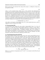
Fig. 11. Pressure variation along the pipeline

Modeling and Simulation for Steady State and Transient Pipe Flow of Condensate Gas

81


Fig. 12. Temperature variation along the pipeline



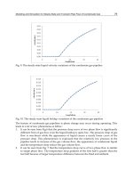
Fig. 13. Velocity of the gas phase variation along the pipeline



Fig. 14. Velocity of the liquid phase variation along the pipeline

Thermodynamics – Kinetics of Dynamic Systems

82

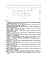
Fig. 15. Liquid hold up variation along the pipeline
Compared with steady state, the following features present.
1.
Fig.11 depicts the pressure along the pipeline drops continuously with time elapsing
after the inlet pressure drops to 10.5MPa at the time of 300s as the changing of
boundary condition.

2.
Fig.12 shows the temperature variation tendency is nearly the same as steady state. The
phenomenon can be explained by the reason that the energy equation is ignored in
order to simplify the transient model. The approximate method is reasonable because
the temperature responses slower than the other parameters.
3.
As depicted in Fig.13, there are abrupt changes of the gas phase velocity at the time of
300s. The opposite direction flow occurs because the pressure at the inlet is lower than
the other sections in the pipeline. However, with the rebuilding of the new steady state,
the velocity tends to reach a new steady state.
4.
Fig.14 shows the velocity variation along the pipeline. Due to the loss of pressure
energy at the inlet, the liquid velocity also drops simultaneously at the time of 300s.
Similar to gas velocity, after 300s, the liquid velocity increases gradually and tends to
reach new steady state with time elapsing.
5.
Due to the same liquid hold up equation is adopted in the steady state and transient
model, the liquid hold up simulated by the transient model and steady state mode has
almost the same tendency (Fig.15). However, the liquid hold up increases because of the
temperature along the pipeline after 300s is lower than that of initial condition.
Sum up, the more details of the results and transient process can be simulated by transient
model. There are still some deficiencies in the model, which should be improved in further
work.
8. Conclusions
In this work, a general model for condensate gas pipeline simulation is built on the basis of
BWRS EOS, continuity equation, momentum equation, energy equation of the gas and
liquid phase. The stratified flow pattern and corresponding constitutive equation are
adopted to simplify the model.
By ignoring the parameters variation with time, the steady state simulation model is
obtained. To solve the model, the four-order Runge - Kutta method and Gaussian

Modeling and Simulation for Steady State and Transient Pipe Flow of Condensate Gas

83
elimination method are used simultaneously. Opposite to steady state model, the transient
model is built with consideration of the parameters variation with time, and the model is
solved by finite difference method. Solving procedures of steady-state and transient models
are presented in detail.
Finally, this work simulated the steady-state and transient operation of a condensate gas
pipeline. The pressures, temperatures, velocity of the gas and liquid phase, liquid hold up
are calculated. The differences between the steady-state and transient state are discussed.
The results show the model and solving method proposed in this work are feasible to
simulate the steady state and transient flow in condensate gas pipeline. Nevertheless, in
order to expand the adaptive range the models, more improvements should be
implemented in future work (Pecenko et al, 2011).
9. Acknowledgment
This paper is a project supported by sub-project of National science and technology major
project of China (No.2008ZX05054) and China National Petroleum Corporation (CNPC)
tackling key subject: Research and Application of Ground Key Technical for CO
2
flooding,
JW10-W18-J2-11-20.
10. References
S. Mokhatab ; William A. Poe & James G. Speight. (2006).Handbook of Natural Gas
Transmission and Processing, Gulf Professional Publishing, ISBN 978-0750677769
Li, C. J. (2008). Natural Gas Transmission by Pipeline, Petroleum Industry Press, ISBN 978-
7502166700, Beijing, China
S. Mokahatab.(2009). Explicit Method Predicts Temperature and Pressure Profiles of Gas-
condensate Pipelines . Energy Sources, Part A. 2009(29): 781-789.
P. Potocnik. (2010). Natural Gas, Sciyo, ISBN 978-953-307-112-1, Rijeka, Crotla.

M. A. Adewumi. & Leksono Mucharam. (1990). Compostional Multiphase Hydrodynamic
Modeling of Gas/Gas-condensate Dispersed Flow. SPE Production Engineering,
Vol.5, No.(2), pp.85-90 ISSN 0885-9221
McCain, W.D. (1990). The Properties of Petroleum Fluids(2
nd
Edition). Pennwell Publishing
Company, ISBN978-0878143351,Tulsa, OK., USA
Estela-Uribe J.F.; Jaramillo J., Salazar M.A. & Trusler J.P.M. (2003). Viriel equation of statefor
natural gas systems. Fluid Phase Equilibria, Vol. 204, No. 2, pp. 169 182.ISSN 0378-
3812
API. (2005). API Technical Databook (7
th
edition), EPCON International and The American
Petroleum Institite, TX,USA
Luis F. Ayala; M. A. Adewumi.(2003). Low liquid loading Multiphase Flow in Nature Gas
Pipelines.Journal of Energy Resources and Technology, Vol.125, No.4, pp. 284-293,
ISSN 1528-8994
Li, Y. X., Feng, S. C.(1998). Studying on transient flow model and value simulation
technology for wet natural gas in pipeline tramsmission. OGST, vol.17, no.5, pp.11-
17, ISSN1000-8241

Thermodynamics – Kinetics of Dynamic Systems

84
Hasan, A.R. & Kabir, C.S.(1992). Gas void fraction in two-phase up-flow in vertical and
inclined annuli. International Journal of Multiphase Flow, Vol.18, No.2, pp.279
–293.
ISSN0301-9322
Li, C. J., Liu E.B. (2009) .The Simulation of Steady Flow in Condensate Gas
Pipeline

，Proceedings of 2009 ASCE International Pipelines and Trenchless Technology
Conference, pp.733-743, ISBN 978-0-7844-1073-8, Shanghai, China, October 19-
21,2009.
Taitel, Y. & Barnea (1995). Stratified three-phase flow in pipes. International Journal of
Multiphase flow, Vol.21, No.2, pp.53-60. ISSN0301-9322
Chen, X. T., Cai, X. D. & Brill, J. P. (1997). Gas-liquid Stratified Wavy Flow in Horizontal
Pipelines, .Journal of Energy Resources and Technology,Vol.119, No.4, pp.209-216 ISSN
1528-8994.
Masella, J.M., Tran, Q.H., Ferre, D., and Pauchon, C.(1998). Transient simulation of two-
phase flows in pipes. Oil Gas Science Technology. Vol. 53, No.6, pp.801
–811 ISSN
1294-4475.
Li, C. J., Jia, W. L., Wu, X.(2010). Water Hammer Analysis for Heated Liquid Transmission
Pipeline with Entrapped Gas Based on Homogeneous Flow Model and Fractional
Flow Model, Proceedings of 2010 IEEE Asia-Pacific Power and Energy Engineering
Conference, ISBN978-1-4244-4813-5, Chengdu, China, March28-21.2010.
A. Pecenko,; L.G.M. van Deurzen. (2011). Non-isothermal two-phase flow with a diffuse-
interface model. International Journal of Multiphase Flow ,Vol.37,No.2,PP.149-165.
ISSN0301-9322
0
Extended Irreversible Thermodynamics in the
Presence of Strong Gravity
Hiromi Saida
Daido University
Japan
1. Introduction
For astrophysical phenomena, especially in the presence of strong gravity, the causality of any
phenomena must be preserved. On the other hand, dissipations, e.g. heat flux and bulk and
shear viscosities, are necessary in understanding transport phenomena even in astrophysical
systems. If one relies on the Navier-Stokes and Fourier laws which we call classic laws of

dissipations, then an infinite speed of propagation of dissipations is concluded (14). (See
appendix 7 for a short summary.) This is a serious problem which we should overcome,
because the infinitely fast propagation of dissipations contradicts a physical requirement that
the propagation speed of dissipations should be less than or equal to the speed of light. This
means the breakdown of causality, which is the reason why the dissipative phenomena have
not been studies well in relativistic situations. Also, the infinitely fast propagation denotes
that, even in non-relativistic case, the classic laws of dissipations can not describe dynamical
behaviors of fluid whose dynamical time scale is comparable with the time scale within which
non-stationary dissipations relax to stationary ones.
Moreover note that, since Navier-Stokes and Fourier laws are independent phenomenological
laws, interaction among dissipations, e.g. the heating of fluid due to viscous flow and the
occurrence of viscous flow due to heat flux, are not explicitly described in those classic laws.
(See appendix 7 for a short summary.) Thus, in order to find a physically reasonable theory of
dissipative fluids, it is expected that not only the finite speed of propagation of dissipations
but also the interaction among dissipations are included in the desired theory of dissipative
fluids.
Problems of the infinite speed of propagation and the absence of interaction among
dissipations can be resolved if we rely not on the classic laws of dissipations but on the
Extended Irreversible Thermodynamics (EIT) (13; 14). The EIT, both in non-relativistic and
relativistic situations, is a causally consistent phenomenology of dissipative fluids including
interaction among dissipations (9). Note that the non-relativistic EIT has some experimental
grounds for laboratory systems (14). Thus, although an observational or experimental
verification of relativistic EIT has not been obtained so far, the EIT is one of the promising
hydrodynamic theories for dissipative fluids even in relativistic situations.
1
1
One may refer to the relativistic hydrodynamics proposed by Israel (11), which describes the causal
propagation of dissipations. However, since the Israel’s hydrodynamics can be regarded as one
approximate formalism of EIT as reviewed in Sec.3, we dare to use the term EIT rather than Israel’s
theory.

4
2 Will-be-set-by-IN-TECH
In astrophysics, the recent advance of technology of astronomical observation realizes a fine
observation whose resolution is close to the view size of celestial objects which are candidates
of black holes (1; 20; 24). (Note that, at present, no certain evidence of the existence of black
hole has been extracted from observational data.) The light detected by our telescope is
emitted by the matter accreting on to the black hole, and the energy of the light is supplied
via the dissipations in accreting matter. Therefore, those observational data should include
signals of dissipative phenomena in strong gravitational field around black hole. We expect
that such general relativistic dissipative phenomena is described by the EIT.
EIT has been used to consider some phenomena in the presence of strong gravity. For
example, Peitz and Appl (23) have used EIT to write down a set of evolution equations
of dissipative fluid and spacetime metric (gravitational field) for stationary axisymmetric
situation. However the Peitz-Appl formulation looks very complicated, and has predicted
no concrete result on astrophysics so far. Another example is the application of EIT to a
dissipative gravitational collapse under the spherical symmetry. Herrera and co-workers (6–8)
constructed some models of dissipative gravitational collapse with some simplification
assumptions. They rearranged the basic equations of EIT into a suitable form, and deduced
some interesting physical implications about dissipative gravitational collapse. But, at
present, there still remain some complexity in Herrera’s system of equations for gravitational
collapse, and it seems not to be applicable to the understanding of observational data of black
hole candidates (1; 20; 24). These facts imply that, in order to extract the signals of strong
gravity from the observational data of black hole candidates, we need a more sophisticated
strategy for the application of EIT to general relativistic dissipative phenomena. In order to
construct the sophisticated strategy, we need to understand the EIT deeply.
Then, this chapter aims to show a comprehensive understanding of EIT. We focus on basic
physical ideas of EIT, and give an important remark on non-equilibrium radiation field
which is not explicitly recognized in the original works and textbook of EIT (9–14). We
try to understand the EIT from the point of view of non-equilibrium physics, because the
EIT is regarded as dissipative hydrodynamics based on the idea that the thermodynamic

state of each fluid element is a non-equilibrium state. (But thorough knowledge of
non-equilibrium thermodynamics and general relativity is not needed in reading this chapter.)
As explained in detail in following sections, the non-equilibrium nature of fluid element
arises from the dissipations which are essentially irreversible processes. Then, non-equilibrium
thermodynamics applicable to each fluid element is constructed in the framework of
EIT, which includes the interaction among dissipations and describes the causal entropy
production process due to the dissipations. Furthermore we point out that the EIT is
applicable also to radiative transfer in optically thick matters (4; 27). However, radiative
transfer in optically thin matters can not be described by EIT, because the non-self-interacting
nature of photons is incompatible with a basic requirement of EIT. This is not explicitely
recognized in standard references of EIT (9–14).
Here let us make two comments: Firstly, note that the EIT can be formulated with
including not only heat and viscosities but also electric current, chemical reaction and
diffusion in multi-component fluids (13; 14). Including all of them raises an inessential
mathematical confusion in our discussions. Therefore, for simplicity of discussions in this
paper, we consider the simple dissipative fluid, which is electrically neutral and chemically inert
single-component dissipative fluid. This means to consider the heat flux, bulk viscosity and
shear viscosity as the dissipations in fluid.
86
Thermodynamics – Kinetics of Dynamic Systems
Extended Irreversible Thermodynamics in the Presence of Strong Gravity 3
As the second comment, we emphasize that the EIT is a phenomenology in which the transport
coefficients are parameters undetermined in the framework of EIT (11; 13; 14). On the other
hand, based on the Grad’s 14-moment approximation method of molecular motion, Israel and
Stewart (12) have obtained the transport coefficients of EIT as functions of thermodynamic
variables. The Israel-Stewart’s transport coefficients are applicable to the molecular kinematic
viscosity. However, it is not clear at present whether those coefficients are applicable
to other mechanisms of dissipations such as fluid turbulent viscosity and the so-called
magneto-rotational-instability (MRI) which are usually considered as the origin of viscosities
in accretion flows onto celestial objects (5; 15; 26). Concerning the MRI, an analysis by Pessah,

Chan, and Psaltis (21; 22) seems to imply that the dissipative effects due to MRI-driven
turbulence can be expressed as some transport coefficients, whose form may be different
from Israel-Stewart’s transport coefficients. Hence, in this chapter, we do not refer to the
Israel-Stewart’s coefficients. We re-formulate the EIT simply as the phenomenology, and
the transport coefficients are the parameters determined empirically through observations
or by underlying fundamental theories of turbulence and/or molecular dynamics. The
determination of transport coefficients and the investigation of micro-processes of transport
phenomena are out of the aim of this chapter. The point of EIT in this chapter is the causality
of dissipations and the interaction among dissipations.
In Sec.2, the basic ideas of EIT is clearly summarized into four assumptions and one
supplemental condition, and a limit of EIT is also reviewed. Sec.3 explains the meanings
of basic quantities and equations of EIT, and also the derivation of basic equations are
summarized so as to be extendable to fluids which are more complicated than the simple
dissipative fluid. Sec.4 is for a remark on a non-equilibrium radiative transfer, of which
the standard references of EIT were not aware. Sec.5 gives a concluding remark on a tacit
understanding which is common to EIT and classic laws of dissipations.
In this chapter, the semicolon “ ; ” denotes the covariant derivative with respect to spacetime
metric, while the comma “ , ” denotes the partial derivative. The definition of covariant
derivative is summarized in appendix 7. (Thorough knowledge of general relativity is
not needed in reading this chapter, but experiences of calculation in special relativity is
preferable.) The unit used throughout is
c
= 1, G = 1, k
B
= 1 . (1)
Since the quantum mechanics is not used in this paper, we do not care about the Planck
constant.
2. Basic assumptions and a supplemental condition of EIT
For the first we summarizes the basis of perfect fluid and classic laws of dissipations. The
theory of perfect fluid is a phenomenology assuming the local equilibrium; each fluid element

is in a thermal equilibrium state. Here note that, exactly speaking, dissipations can not
exist in thermal equilibrium states. Thus the local equilibrium assumption is incompatible
with the dissipative phenomena which are essentially the irreversible and entropy producing
processes. By that assumption, the basic equations of perfect fluid do not include any
dissipation, and any fluid element in perfect fluid evolves adiabatically. No entropy
production arises in the fluid element of perfect fluid (19). Furthermore, recall that the classic
laws of dissipations (Navier-Stokes and Fourier laws) are also the phenomenologies assuming
87
Extended Irreversible Thermodynamics in the Presence of Strong Gravity
4 Will-be-set-by-IN-TECH
the local equilibrium. Therefore, the classic laws of dissipations lead inevitably some
unphysical conclusions, one of which is the infinitely fast propagation of dissipations (13; 14).
From the above, it is recognized that we should replace the local equilibrium assumption with
the idea of local non
-equilibrium in order to obtain a physically consistent theory of dissipative
phenomena. This means to consider that the fluid element is in a non-equilibrium state. A
phenomenology of dissipative irreversible hydrodynamics, under the local non-equilibrium
assumption, is called the Extended Irreversible Thermodynamics (EIT).
2
The basic assumptions
of EIT can be summarized into four statements. As discussed above, the first one is as follows:
Assumption 1 (Local Non-equilibrium). The dissipative fluid under consideration is in “local”
non-equilibrium states. This means that each fluid element is in a non-equilibrium state, but the
non-equilibrium state of one fluid element is not necessarily the same with the non-equilibrium state of
the other fluid element.

Due to this assumption, it is necessary for the EIT to formulate a non-equilibrium
thermodynamics to describe thermodynamic state of each fluid element. In order to formulate
it, we must specify the state variables which are suitable for characterizing non-equilibrium
states. The second assumption of EIT is on the specification of suitable state variables for

non-equilibrium states of fluid elements:
Assumption 2 (Non-equilibrium thermodynamic state variables). The state variables which
characterize the non-equilibrium states are distinguished into two categories;
1st category (Non-equilibrium Vestiges) The state variables in this category do not necessarily
vanish at the local equilibrium limit of fluid. These are the variables specified already in equilibrium
thermodynamics, e.g. the temperature, internal energy, pressure, entropy and so on.
2nd category (Dissipative Fluxes) The state variables in this category should vanish at the local
equilibrium limit of fluid. These are, in the framework of EIT of simple dissipative fluid, the “heat
flux”, “bulk viscosity”, “shear viscosity” and their thermodynamic conjugate state variables. (e.g.
thermodynamic conjugate to entropy S is temperature T
≡ ∂E/∂S, where E is internal energy.
Similarly, thermodynamic conjugate to bulk viscosity Π can be given by ∂E/∂Π, where E is now
“non-equilibrium” internal energy.)

Note that the terminology “non-equilibrium vestige” is a coined word introduced by the
present author, and not a common word in the study on EIT. But let us dare to use the term
“non-equilibrium vestige” to explain clearly the idea of EIT.
Next, recall that, in the ordinary equilibrium thermodynamics, the number of independent
state variables is two for closed systems which conserve the number of constituent particles,
and three for open systems in which the number of constituent particles changes. For
non-equilibrium states of dissipative fluid elements, it seems to be natural that the number
of independent non-equilibrium vestiges is the same with that of state variables in ordinary
equilibrium thermodynamics. On the other hand, in the classic laws of dissipations which are
summarized in Eq.(46) in appendix 7, the dissipative fluxes such as heat flux and viscosities
were not independent variables, but some functions of fluid velocity and local equilibrium
state variables such as temperature and pressure. However in the EIT, the dissipative fluxes
2
Although the EIT is a dissipative “hydrodynamics”, it is named “thermodynamics”. This name puts
emphasis on the replacement of local equilibrium idea with local non-equilibrium one, which is a
revolution in thermodynamic treatment of fluid element.

88
Thermodynamics – Kinetics of Dynamic Systems
Extended Irreversible Thermodynamics in the Presence of Strong Gravity 5
are assumed to be independent of fluid velocity and non-equilibrium vestiges. Then, the third
assumption of EIT is on the number of independent state variables:
Assumption 3 (Number of Independent State Variables). The number of independent
non-equilibrium vestiges is the same with the ordinary thermodynamics (two for closed system and
three for open system). Furthermore, EIT assumes that the number of independent dissipative fluxes
are three. For example, we can regard the heat flux, bulk viscosity and shear viscosity are independent
dissipative fluxes.

3
Mathematically, the independent state variables can be regarded as a “coordinate system”
in the space which consists of thermodynamic states. A set of values of the coordinates
corresponds to a particular non-equilibrium state. This means that the set of values of
independent state variables is uniquely determined for each non-equilibrium state, and
different non-equilibrium states have different sets of values of independent state variables.
Assumption 3 implies the existence of non-equilibrium equations of state, from which we
can obtain “dependent” state variables. Concrete forms of non-equilibrium equations of state
should be determined by experiments or micro-scopic theories of dissipative fluids. Given the
non-equilibrium equations of state, we can consider a case that the non-equilibrium entropy,
S
ne
, is a dependent state variable. In this case, S
ne
depends on an independent dissipative
flux, e.g. the bulk viscosity Π. Obviously, since Π is one of the dissipative fluxes, the partial
derivative, ∂S
ne
/∂Π, has no counter-part in ordinary equilibrium thermodynamics. This

implies that ∂S
ne
/∂Π is a member not of non-equilibrium vestiges but of dissipative fluxes.
Hence, by the assumption 2, we find that the partial derivative of dependent state variable by
an independent dissipative flux should vanish at local equilibrium limit of fluid,
∂
[non-equilibrium dependent state variable]
∂[independent dissipative flux]
→
0 as [independent dissipative fluxes] → 0.
(2)
The assumptions 1, 2 and 3 can be regarded as the zeroth law of non-equilibrium
thermodynamics formulated in the EIT, which prescribes the existence and basic properties
of local non-equilibrium states of dissipative fluids. In the relativistic formulation of EIT, the
state variables are gathered in the energy-momentum tensor, T
μν
. The definition of T
μν
will
be shown in next section.
Here note that, because EIT is a “hydrodynamics”, we should consider not only
non-equilibrium thermodynamic state variables but also a dynamical variable, the fluid
velocity. As will be shown in next section, the basic equations of EIT determine not only
non-equilibrium state variables but also the dynamical variable (velocity) of fluid element,
when initial and boundary conditions are specified. Hence, via the basic equations, the fluid
velocity can be regarded as a function of thermodynamic state variables of fluid elements.
The evolution equations of fluid velocity and non-equilibrium vestiges are given by the
conservation laws of mass current vector and energy-momentum tensor as will be shown
3
As an advanced remark, recall that, in ordinary equilibrium thermodynamics, if there is an external field

such as a magnetic field applied on a magnetized gas, then the number of independent state variables
increases for both closed and open systems. Usually, the external field itself can be regarded as an
additional independent state variable. The same is true of the number of independent non-equilibrium
vestiges. In this paper, we consider no external field other than the external gravity (the metric), and the
metric can be regarded as an additional independent non-equilibrium vestige. However, for simplicity
and in order to focus our attention to intrinsic state variables of non-equilibrium states, we do not
explicitly show the metric as an independent state variable in all discussions in this paper.
89
Extended Irreversible Thermodynamics in the Presence of Strong Gravity
6 Will-be-set-by-IN-TECH
in next section. Then, in order to obtain the evolution equations of dissipative fluxes, we need
guiding principles. In the EIT, such guiding principles are the second law of thermodynamics
and the phenomenological requirement based on laboratory experiments summarized in
appendix 7. The fourth assumption of EIT is on these guiding principles:
Assumption 4 (Second Law and Phenomenology). The self-production rate of entropy by a fluid
element at spacetime point x, σ
s
(x), is defined by the divergence of non-equilibrium entropy current
vector, σ
s
:= S
μ
ne
;μ
, where the detail of S
μ
ne
is not necessary at present and shown in Sec.3.2.
Concerning σ
s

, EIT assumes the followings:
(4-a) Entropy production rate is non-negative, σ
s
≥ 0 (2nd law).
(4-b) Entropy production rate is expressed by the bilinear form,
σ
s
= [Dissipative Flux] ×[Thermodynamic force] , (3)
where, as explained below, the “thermodynamic force” is given by some gradients of state variables
which raises a dissipative flux, and the functional form of thermodynamic force should be consistent
with existing phenomenologies summarized in appendix 7. Concrete forms of them are derived in
Sec.3.2.

The notion of thermodynamic force in requirement (4-b) is not a particular property of EIT.
Indeed, the thermodynamic force has already been known in classic laws of dissipations. For
example, the Fourier law,

q = −λ

∇
T, implies that the temperature gradient, −

∇T, is the
thermodynamic force which raises the heat flux,

q, where λ is the heat conductivity. Also, it
is already known for the Fourier law that the entropy production rate is given by the bilinear
form,

q · (−


∇T)=q
2
/λ ≥ 0, where

q and −

∇T corresponds respectively to the dissipative
flux and thermodynamic force in the above requirement (4-b) (13; 14). The assumption 4 is
a simple extension of the local equilibrium theory to the local non-equilibrium theory. The
causality of dissipative phenomena is not retained by solely the assumption 4. Also, the
inclusion of interaction among dissipative fluxes is not achieved by solely the assumption 4.
The point of preservation of causality and inclusion of interaction among dissipations is
the definition of non-equilibrium entropy current, S
μ
ne
. As explained in next section, once
an appropriate definition of S
μ
ne
is given, the assumption 4 together with the other three
assumptions yields the evolution equations of dissipative fluxes which retain the causality
of dissipative phenomena and includes the interaction among dissipative fluxes.
To find the appropriate definition of S
μ
ne
, it should be noted that, unfortunately, some critical
problems have been found for the cases of strong dissipative fluxes; e.g. the uniqueness of
non-equilibrium temperature, T
ne

, and non-equilibrium pressure, p
ne
, can not be established
in the present status of EIT (13; 14). These problems are the very difficult issues in
non-equilibrium physics. At present, the EIT seems not to be applicable to a non-equilibrium
state with strong dissipations. However, we can expect that, by restricting our discussion
to the case of weak dissipative fluxes, the difficult problems in non-equilibrium physics is
avoided and a well-defined entropy current, S
μ
ne
, is obtained. This expectation is realized by
adopting a perturbative method summarized in the following supplemental condition:
Supplemental Condition 1 (Second Order Approximation of Equations of State). Restrict our
interest to the non-equilibrium states which are not so far from equilibrium states. This means that
the dissipative fluxes are not very strong. Quantitatively, we consider the cases that the strength of
dissipative fluxes is limited so that the “second order approximation of equations of state” is appropriate:
90
Thermodynamics – Kinetics of Dynamic Systems
Extended Irreversible Thermodynamics in the Presence of Strong Gravity 7
Some examples about non-equilibrium specific entropy, s
ne
, and non-equilibrium temperature, T
ne
,
are (13; 14)
s
ne
(ε
ne
, V

ne
, q
μ
, Π,
◦
Π
μν
)=s
eq
(ε
eq
, V
eq
)+[2nd order terms of q
μ
, Π and
◦
Π
μν
] (4a)
T
ne
(ε
ne
, V
ne
, q
μ
, Π,
◦

Π
μν
)=T
eq
(ε
eq
, V
eq
)+[2nd order terms of q
μ
, Π and
◦
Π
μν
] , (4b)
where we choose ε
ne
,V
ne
,q
μ
, Π and
◦
Π
μν
as the independent state variables of non-equilibrium state
of each fluid element, and suffix “ne” denotes “non-equilibrium”. The quantities ε
ne
and V
ne

are
respectively the non-equilibrium specific internal energy and specific volume which are non-equilibrium
vestiges, and q
μ
, Π and
◦
Π
μν
are respectively the heat flux, bulk viscosity and shear viscosity which
are dissipative fluxes. In Eq.(4), the quantities with suffix “eq” are the state variables of “fiducial
equilibrium state”, which is defined as the equilibrium state of fluid element of an imaginary perfect
fluid (non-dissipative fluid) possessing the same value of fluid velocity and rest mass density with our
actual dissipative fluid. Then, s
eq
(ε
eq
, V
eq
) and T
eq
(ε
eq
, V
eq
) in Eq.(4) are given by the equations
of state for fiducial equilibrium state. Note that, under the second order approximation (4), the
“non-equilibrium vestiges” are reduced to the state variables of fiducial equilibrium state. Also note
that, because of Eq.(2), no first order term of independent dissipative flux appears in Eq.(4).In
summary, Eq.(4) is the expansion of non-equilibrium equations of state about the fiducial equilibrium
state up to the second order of independent dissipative fluxes. Thus, the dissipative fluxes under this

condition are regarded as a non-equilibrium thermodynamic perturbation on the fiducial equilibrium
state.

As will be shown in Sec.3.2, the basic equations of EIT is derived using not only the
assumptions 1
∼ 4 but also the supplemental condition 1. Then, one may regard the
supplemental condition 1 as one of basic assumptions of EIT. However, in the study on
non-equilibrium physics, there seem to be some efforts to go beyond the second order
approximation required in supplemental condition 1 (13; 14). Thus, in this paper, let us
understand that the supplemental condition 1 is not a basic assumption but a supplemental
condition to make the four basic assumptions work well.
A quantitative estimate of the strength of dissipative fluxes for a particular situation has been
examined by Hiscock and Lindblom (10). They investigated an ultra-relativistic gas including
only a heat flux under the planar symmetry. We can recognize from the Hiscock-Lindblom’s
analysis that, for the system they investigated, the second order approximation of equations
of state such as Eq.(4) is valid for the heat flux, q
μ
, satisfying the inequality,
q
ρ
eq
ε
eq
 0.08898 , (5)
where q :
=

q
μ
q

μ
. Note that the density of internal energy of fiducial equilibrium state,
ρ
eq
ε
eq
, includes the rest mass energy of the fluid. Therefore, the inequality (5) implies that the
supplemental condition 1 is appropriate when the heat flux is less than a few percent of the
internal energy density including mass energy.
91
Extended Irreversible Thermodynamics in the Presence of Strong Gravity
8 Will-be-set-by-IN-TECH
3. Basic quantities and basic equations of EIT
3.1 Meanings of basic quantities and equations
The basic quantities of dissipative fluid in the framework of EIT:
u
μ
(x) : velocity field of dissipative fluid (four-velocity of dissipative fluid element)
ρ
ne
(x) : rest mass density for non-equilibrium state
ε
ne
(x) : non-equilibrium specific internal energy (internal energy per unit rest mass)
p
ne
(x) : non-equilibrium pressure
T
ne
(x) : non-equilibrium temperature

q
μ
(x) : heat flux vector
Π
(x) : bulk viscosity
◦
Π
μν
(x) : shear viscosity tensor
g
μν
(x) : spacetime metric tensor .
The specific volume, V
ne
(volume per unit rest mass), which is one of non-equilibrium
vestiges, is defined by
V
ne
(x) := ρ
ne
(x)
−1
. (6)
These quantities will appear in the basic equations of EIT.
4
All of the above quantities are the
“field” quantities defined on spacetime manifold, and x denotes the coordinate variables on
spacetime. Quantities ρ
ne
, ε

ne
, p
ne
and T
ne
are non-equilibrium vestiges, and quantities q
μ
, Π
and
◦
Π
μν
are the dissipative fluxes (see assumption 2).
Note that, it is possible to determine the values of u
μ
and ρ
ne
without referring to the other
thermodynamic state variables. The fluid velocity, u
μ
, is simply defined as the average
four-velocity of constituent particles in a fluid element. This definition of fluid velocity is
called the N-frame by Israel (11). The rest mass density, ρ
ne
, is simply defined by the rest
mass per unit three-volume perpendicular to u
μ
. Because u
μ
and ρ

ne
are determined without
the knowledge of local non-equilibrium state, the fiducial equilibrium state is defined with
referring to u
μ
and ρ
ne
as explained in the supplemental condition 1.
Then, the rest mass current vector, J
μ
, is defined as
J
μ
:= ρ
ne
u
μ
. (7)
The relations between the basic quantities and energy-momentum tensor, T
μν
, of dissipative
fluid are
ρ
ne
ε
ne
= u
α
u
β

T
αβ
(8a)
q
μ
= −Δ
μα
u
β
T
αβ
(8b)
p
ne
+ Π =
1
3
Δ
αβ
T
αβ
(8c)
◦
Π
μν
=

Δ
μα
Δ

νβ
−
1
3
Δ
μν
Δ
αβ

T
αβ
, (8d)
4
In this paper, following the textbook of EIT (13; 14), we use the specific scalar quantities, which are
defined per unit rest mass. On the other hand, some references of EIT (9–12) use the density of those
scalar quantities, which are defined per unit three-volume perpendicular to u
μ
.
92
Thermodynamics – Kinetics of Dynamic Systems
Extended Irreversible Thermodynamics in the Presence of Strong Gravity 9
where Δ
μν
is a projection tensor on perpendicular direction to u
μ
defined as
Δ
μν
:= u
μ

u
ν
+ g
μν
. (9)
These relations (8) are simply the mathematically general decomposition of symmetric tensor
T
μν
. For the observer comoving with the fluid, ρ
ne
ε
ne
is the temporal-temporal component
of T
μν
, q
μ
the temporal-spatial component of T
μν
, p
ne
+ Π the trace part of spatial-spatial
component of T
μν
, and
◦
Π
μν
the trace-less part of spatial-spatial component of T
μν

. Here,
note that p
ne
and Π can not be distinguished by solely the relation (8c). However, we can
distinguish p
ne
and Π, when the equations of state are specified in which the pressure and
bulk viscosity play different roles. Furthermore, as explained below, the basic equations of EIT
are formulated so that p
ne
and Π are distinguished and obey different evolution equations.
Thus, we find that, given the basic quantities of dissipative fluid, the energy-momentum
tensor can be defined as
T
μν
:= ρ
ne
ε
ne
u
μ
u
ν
+ 2 u
(μ
q
ν)
+(p
ne
+ Π) Δ

μν
+
◦
Π
μν
, (10)
where the symmetrization u
(μ
q
ν)
is defined as
u
(μ
q
ν)
:=
1
2
(
u
μ
q
ν
+ u
ν
q
μ
)
. (11)
From the normalization of u

μ
, symmetry T
μν
= T
νμ
and relations (8), we find some constraints
on basic quantities of dissipative fluid (11; 12):
u
μ
u
μ
= −1 (12a)
u
μ
q
μ
= 0 (12b)
◦
Π
μν
=
◦
Π
νμ
(12c)
u
ν
◦
Π
μν

= 0 (12d)
◦
Π
μ
μ
= 0 . (12e)
Of course, the metric is symmetric g
μν
= g
νμ
. These constraints denote that the independent
quantities are ten components of g
μν
, three components of u
μ
, three components of q
μ
, five
components of
◦
Π
μν
, five scalars ρ
ne
, ε
ne
, p
ne
, T
ne

and Π. Here recall that, according to
assumption 3, some non-equilibrium equations of state should exist in order to guarantee
the number of independent state variables. Such equations of state may be understood as
constraints on state variables.
The ten components of metric g
μν
are determined by the Einstein equation,
G
μν
= 8π T
μν
, (13)
where G
μν
:= R
μν
−(1/2) R
α
α
g
μν
is the Einstein tensor, and R
μν
is the Ricci curvature tensor.
Hence, in the framework of EIT, we need evolution equations to determine the remaining
independent sixteen quantities u
μ
, q
μ
,

◦
Π
μν
, ρ
ne
, ε
ne
, p
ne
, T
ne
and Π.
Next, let us summarize the sixteen basic equations of EIT other than the Einstein equation.
Hereafter, for simplicity, we omit the suffix “eq” of the state variables of fiducial equilibrium
state,
ρ :
= ρ
eq
, ε := ε
eq
, p := p
eq
, T := T
eq
, s := s
eq
. (14)
93
Extended Irreversible Thermodynamics in the Presence of Strong Gravity
10 Will-be-set-by-IN-TECH

The five of the desired sixteen equations of EIT are given by the conservation law of rest mass,
J
μ
;μ
= 0, and that of energy-momentum, T
μν
;ν
= 0:
•
ρ + ρ u
μ
;μ
= 0 (15a)
ρ

•
ε +(p + Π)
•
V

= −q
μ
;μ
−q
μ
•
u
μ
−
◦

Π
μν
u
μ ; ν
(15b)
(
ρε+ p + Π
)
•
u
μ
= −
•
q
μ
+q
α
•
u
α
u
μ
−u
α
;α
q
μ
−q
α
u

μ
;α
−

(p + Π)
,α
+
◦
Π
β
α ;β

Δ
αμ
, (15c)
where the non-equilibrium vestiges are reduced to the state variables of fiducial equilibrium
state due to the supplemental condition 1, and Eqs.(15) retain only the first order dissipative
corrections to the evolution equations of perfect fluid. Here,
•
Q is the Lagrange derivative of
quantity Q defined by
•
Q := u
μ
Q
;μ
. (16)
And, Eq.(15a) is given by J
μ
;μ

= 0 which is the continuity equation (mass conservation) ,
Eq.(15b) is given by u
μ
T
μν
;ν
= 0 which is the energy conservation and corresponds to the first
law of non-equilibrium thermodynamics in the EIT, and Eq.(15c) is given by Δ
μα
T
β
α ;β
= 0
which is the Euler equation (equation of motion of dissipative fluid).
Here, let us note the relativistic effects and number of independent equations. The relativistic
effects are q
μ
•
u
μ
in Eq.(15b), and (p + Π)
•
u
μ
and the terms including q
μ
in Eq.(15c).
Those terms do not appear in non-relativistic EIT (13; 14). And, due to the constraint
of normalization (12a), three components of Euler equation (15c) are independent, and
one component is dependent. Totally, the five equations are independent in the set of

equations (15).
The nine of desired sixteen equations of EIT are the evolution equations of dissipative
fluxes, whose derivation are reviewed in next subsection using the assumptions 1
∼ 4 and
supplemental condition 1. According the next subsection or references of EIT (9; 11; 13; 14),
the evolution equations of dissipations are
τ
h
•
q
μ
= −

1
+ λ T
2

τ
h
2λT
2
u
ν

;ν

q
μ
−λ T
•

u
μ
+ τ
h
(q
ν
•
u
ν
) u
μ
−λ Δ
μν

T
,ν
− T
2

β
hb
Π
,ν
+(1 −γ
hb
) Π β
bh ,ν
+ β
hs
◦

Π
α
ν ;α
+(1 −γ
hs
) β
hs ,α
◦
Π
α
ν
}
]
(17a)
τ
b
•
Π = −

1
+ ζ T

τ
b
2ζT
u
μ

;μ


Π
−ζ u
μ
;μ
+ ζ T

β
hb
q
μ
;μ
+ γ
hb
q
μ
β
hb ,μ

(17b)
τ
s

◦
Π
μν

•
= −

1

+ 2 η T

τ
s
4ηT
u
α

;α

◦
Π
μν
+ 2 τ
s
•
u
α
◦
Π
α (μ
u
ν)
−2 η [[ u
μ;ν
− T

β
hs
q

μ;ν
+ γ
hs
β
,μ
hs
q
ν

]]
◦
, (17c)
94
Thermodynamics – Kinetics of Dynamic Systems
Extended Irreversible Thermodynamics in the Presence of Strong Gravity 11
where the symbolic operation [[ A
μν
]]
◦
in the last term in Eq.(17c) denotes the traceless
symmetrization of a tensor A
μν
in the perpendicular direction to u
μ
,
[[ A
μν
]]
◦
:= Δ

μα
Δ
νβ
A
(αβ)
−
1
3
Δ
μν
Δ
αβ
A
αβ
. (18)
We find
◦
Π
μν
=[[T
μν
]]
◦
by Eq.(8d), and [[
◦
Π
μν
]]
◦
=

◦
Π
μν
.
The meanings of coefficients appearing in Eq.(17) are:
λ : heat conductivity
ζ : bulk viscous rate
η : shear viscous rate
τ
h
: relaxation time of heat flux q
μ
τ
b
: relaxation time of bulk viscosity Π
τ
s
: relaxation time of shear viscosity
◦
Π
μν
,
(19a)
and
β
hb
: interaction coefficient between dissipative fluxes q
μ
and Π
β

hs
: interaction coefficient between dissipative fluxes q
μ
and
◦
Π
μν
γ
hb
: interaction coefficient between thermodynamic forces of q
μ
and Π
γ
hs
: interaction coefficient between thermodynamic forces of q
μ
and
◦
Π
μν
,
(19b)
where the thermodynamic forces of q
μ
, Π and
◦
Π
μν
, which we express respectively by symbols
X

μ
h
, X
b
and X
μν
s
, are the quantities appearing in the bilinear form (3) as σ
s
= q
μ
X
μ
h
+ Π X
h
+
◦
Π
μν
X
μν
s
.
In general, the above ten coefficients are functions of state variables of fiducial equilibrium
state. Those functional forms should be determined by some micro-scopic theory or
experiment of dissipative fluxes, but it is out of the scop of this paper.
The coefficients in list (19a) are already known in the classic laws of dissipations and
Maxwell-Cattaneo laws summarized in appendix 7. Note that the existence of relaxation
times of dissipative fluxes make the evolution equations (17) retain the causality of dissipative

phenomena. The relaxation time, τ
h
, is the time scale in which a non-stationary heat flux
relaxes to a stationary heat flux. The other relaxation times, τ
b
and τ
s
, have the same meaning
for viscosities. These are positive by definition,
τ
h
> 0, τ
b
> 0, τ
s
> 0 . (20)
Concerning the transport coefficients, λ, ζ and η, the non-negativity of them is obtained by
the requirement (4-a) in assumption 4 as explained in next subsection,
λ
≥ 0, ζ ≥ 0, η ≥ 0 . (21)
The coefficients in list (19b) denotes that the EIT includes the interaction among dissipative
fluxes, while the classic laws of dissipations and Maxwell-Cattaneo laws do not. (See
appendix 7 for a short summary.) Concerning the interaction among dissipative fluxes,
Israel (11) has introduced an approximation into the evolution equations (17). Israel ignores
the gradients of fiducial equilibrium state variables, as summarized in the end of next
95
Extended Irreversible Thermodynamics in the Presence of Strong Gravity
12 Will-be-set-by-IN-TECH
subsection. Then, Eq.(17) can be slightly simplified by discarding terms including the
gradients. Those simplified equations are shown in Eq.(34).

Given the meanings of all quantities which appear in Eq.(17), we can recognize
a thermodynamical feature of Eq.(17). Recall that the dissipative phenomena are
thermodynamically irreversible processes. Then, reflecting the irreversible nature, the evolution
equations of dissipative fluxes (17) are not time-reversal invariant, i.e. Eq. (17) are not
invariant under the replacement, u
μ
→−u
μ
and q
μ
→−q
μ
.
Here, let us note the relativistic effects and number of independent evolution equations of
dissipative fluxes. The relativistic effects are three terms including
•
u
μ
and three terms of
the form
( u
μ
)
;μ
in right-hand sides of Eq.(17). Those terms disappear in non-relativistic
EIT (13; 14). And, due to the constraints in Eqs.(12) except Eq.(12a), the three components of
evolution equation (17a) and five components of evolution equation (17c) are independent.
Totally, nine equations are independent in the set of equations (17).
From the above, we have fourteen independent evolution equations in Eqs.(15) and (17). We
need the other two equations to determine the sixteen quantities which appear in Eqs.(15)

and (17). Those two equations, under the supplemental condition 1, are the equations of state
of fiducial equilibrium state. They are expressed, for example, as
p
= p(ε, V) , T = T(ε, V) . (22)
The concrete forms of Eq.(22) can not be specified unless the dissipative matter composing the
fluid is specified.
In summary, the basic equations of EIT, under the supplemental condition 1, are Eqs.(15), (17)
and (22) with constraints (12), and furthermore the Einstein equation (13) for the evolution of
metric. With those basic equations, it has already been known that the causality is retained for
dissipative fluids which are thermodynamically stable. Here the “thermodynamic stability”
means that, for example, the heat capacity and isothermal compressibility are positive (9). The
positive heat capacity and positive isothermal compressibility are the very usual and normal
property of real materials. We recognize that the EIT is a causal hydrodynamics for dissipative
fluids made of ordinary matters.
3.2 Derivation of evolution equations of dissipations
Let us proceed to the derivation of Eqs.(17). In order to obtain them, we refer to the
assumption 4 and need the non-equilibrium entropy current vector, S
μ
ne
. The entropy current,
S
μ
ne
, is a member of dissipative fluxes (see assumption 2). Hereafter, we choose q
μ
, Π and
◦
Π
μν
as the three independent dissipative fluxes (see assumption 3). Then S

μ
ne
is a dependent state
variable and should be expanded up to the second order of independent dissipative fluxes
under the supplemental condition 1 (11; 13; 14),
S
μ
ne
:= ρ
ne
s
ne
u
μ
+
1
T
q
μ
+ β
hb
Π q
μ
+ β
hs
q
ν
◦
Π
νμ

, (23)
where we assume the isotropic equations of state which will be explained below, the factor
ρ
ne
s
ne
in the first term is expanded up to the second order of independent dissipative fluxes
due to the supplemental condition 1, the second term T
−1
q
μ
is the first order term of heat flux
due to the meaning of “heat” already known in the ordinary equilibrium thermodynamics,
and the third and fourth terms express the interactions between heat flux and viscosities
as noted in list (19b). These interactions between heat and viscosities are one of significant
96
Thermodynamics – Kinetics of Dynamic Systems
Extended Irreversible Thermodynamics in the Presence of Strong Gravity 13
properties of EIT, while classic laws of dissipations and Maxwell-Cattaneo laws summarized
in appendix 7 do not include these interactions.
Before proceeding to the discussion on the bilinear form of entropy production rate, we should
give two remarks on Eq.(23): First remark is on the first order term of heat flux, T
−1
q
μ
. One
may think that this term is inconsistent with Eq.(2), since the differential, ∂
(T
−1
q

μ
)/∂q
μ
=
T
−1
, does not vanish at local equilibrium limit. However, recall that the fluid velocity, u
μ
,
depends on the dissipative fluxes. Then, we expect a relation, ρ
ne
s
ne
(∂u
μ
/∂q
μ
)=−T
−1
,by
which Eq.(2) is satisfied. The evolution equations of EIT should yield u
μ
so that S
μ
ne
satisfies
Eq.(2).
Second remark is on the second order terms of dissipative fluxes in Eq.(23), which reflect the
notion of isotropic equations of state. Considering a general form of those terms relates to
considering a general form of non-equilibrium equations of state. In general, there may be

a possibility for non-equilibrium state that equations of state depend on a special direction,
e.g. a direction of spinor of constituent particles, a direction of defect of crystal structure in
a solid or liquid crystal system, a direction originated from some turbulent structure, and
so on, which reflect a rather micro-scopic structure of the system under consideration. If a
dependence on such a special direction arises in non-equilibrium equations of state, then the
entropy current, S
μ
ne
, may depend on some tensors reflecting the special direction, and its
most general form up to the second order of independent dissipative fluxes is (9; 12–14)
S
μ
ne
:= Eq.(23) + β

hb
Π A
μα
q
α
+ β

hs
B
αβ
q
α
◦
Π
βμ

+ β

hs
C
αβγμ
q
α
◦
Π
βγ
+ β

hs
D
αβ
◦
Π
αβ
q
μ
+β

bs
Π
◦
Π
μα
E
α
+ β


hs
Π
◦
Π
αβ
F
αβμ
+ β

bb
Π
2
G
μ
+ β

hh
H
α
q
α
q
μ
+ β

hh
I
αβμ
q

α
q
β
+β

ss
J
αβγ
◦
Π
αβ
◦
Π
γμ
+ β

ss
K
μ
◦
Π
αβ
◦
Π
αβ
,
(24)
where A
μν
···K

μ
are the tensors reflecting the special direction. Although Eq.(24) is the most
general form of S
μ
ne
, the inclusion of such a special direction raises an inessential mathematical
confusion in following discussions.
5
Furthermore, recall that, usually, such a special direction
of micro-scopic structure does not appear in ordinary equilibrium thermodynamics which
describes the macro-scopic properties of the system. Thus, under the supplemental condition 1
which restricts our attention to non-equilibrium states near equilibrium states, it may be
expected that such a special direction does not appear in non-equilibrium equations of state.
Let us assume the isotropic equations of state in which the directional dependence does not exist,
and adopt Eq.(23) as the equation of state for S
μ
ne
.
6
Here, since a non-equilibrium factor, ρ
ne
s
ne
, appears in Eq.(23), we need to show
the non-equilibrium equation of state for it. Adopting the isotropic assumption, the
non-equilibrium equation of state (4a) for s
ne
becomes (13; 14),
ρ
ne

s
ne
(ε
ne
, V
ne
, q
μ
, Π,
◦
Π
μν
)=ρ s(ε, V) − a
h
q
μ
q
μ
− a
b
Π
2
− a
s
◦
Π
μν
◦
Π
μν

, (25)
5
There may be a possibility that the factor tensors are gradients of fiducial equilibrium state variable, e.g.
K
μ
∝ ε
,μ
ne
. Those gradients are not micro-scopic quantity. However, in thermodynamics, it is naturally
expected that equations of state do not depend on gradients of state variables but depend only on the
state variables themselves. Furthermore, if complete nonequilibrium equations of state do not include
gradients of state variables, their Tayler expansion can not include gradients in the expansion factors.
6
When one specifies the material composing the dissipative fluid, and if its non-equilibrium equations
of state have some directional dependence, then the same procedure given in Sec. 3.2 provides the basic
equations of EIT depending on a special direction.
97
Extended Irreversible Thermodynamics in the Presence of Strong Gravity
14 Will-be-set-by-IN-TECH
where the suffix “eq” of state variables of fiducial equilibrium state in right-hand side
are omitted as noted in Eq.(14), the expansion coefficients, a
h
, a
b
and a
s
, are functions of
fiducial equilibrium state variables, and the minus sign in front of them expresses that the
non-equilibrium entropy is less than the fiducial equilibrium entropy. Concrete forms of those
coefficients will be obtained below.

On the specific entropy of fiducial equilibrium state, s
(ε, V), the first law of thermodynamics
for fiducial equilibrium state is important in calculating the bilinear form of entropy
production rate (3), T
•
s =
•
ε + p
•
V. Combining the first law of fiducial equilibrium state with
the energy conservation (15b), we find
ρ
•
s +
1
T
q
μ
;μ
= −
1
T

u
μ
;μ
Π +
•
u
μ

q
μ
+ u
μ;ν
◦
Π
μν

, (26)
where Eq.(15a) is used in deriving the first term in right-hand side. This relation is used in
following calculations.
Given the above preparation, we can proceed to calculation of the bilinear form of entropy
production rate. The entropy production rate is defined as the divergence, σ
s
:= S
μ
ne ;¯
,as
already given in assumption 4. Then, according to Eq.(3), σ
s
should be rearranged to the
bilinear form (13; 14),
σ
s
:= S
μ
ne ;¯
= q
μ
X

μ
h
+ Π X
b
+
◦
Π
μν
X
μν
s
, (27)
where the factors, X
μ
h
, X
b
and X
μν
s
, are the thermodynamic forces. To determine the concrete
forms of thermodynamic forces, let us carry out the calculation of the divergence, S
μ
ne ;¯
of
Eq.(23). We find immediately that the divergence includes the differentials of β
hb
and β
hs
as,

S
μ
ne ;¯
= Π q
μ
β
hb
,μ
+
◦
Π
μν
q
ν
β
hs
,μ
+ ···. The assumptions 1 ∼4 can not determine whether the
term Π q
μ
β
hb
,μ
should be put into q
μ
X
μ
h
or Π X
b

in Eq.(27), and whether the term
◦
Π
μν
q
ν
β
hs
,μ
should be put into q
μ
X
μ
h
or
◦
Π
μν
X
μν
s
in Eq.(27). Hence, we introduce additional factors, γ
hb
and γ
hs
, to divide those terms so that the three terms in Eq.(27) become (9)
q
μ
X
μ

h
= q
μ

(1 − γ
hb
) Π β
,μ
hb
+(1 −γ
hs
)
◦
Π
μν
β
hs
,ν
+ ···

Π X
b
= Π

γ
hb
q
μ
β
hb

,μ
+ ···

◦
Π
μν
X
μν
s
=
◦
Π
μν

γ
hs
q
ν
β
,μ
hs
+ ···

.
(28)
Note that γ
hb
and γ
hs
are included in thermodynamic forces. The factor γ

hb
connects X
μ
h
and
X
b
, and γ
hs
connects X
μ
h
and X
μν
s
. Therefore, we can understand that these factors, γ
hb
and
γ
hs
, are the kind of interaction coefficients among thermodynamic forces as noted in list (19b).
Then, using Eqs.(25) and (26), we obtain the concrete forms of X’s,
X
μ
h
= −2 a
h
•
q
μ

−

a
h
u
α

;α
u
μ
−
1
T
•
u
μ
−
1
T
2
T
,μ
+β
hb
Π
,μ
+(1 −γ
hb
) β
,μ

hb
Π + β
hs
◦
Π
μα
;α
+(1 −γ
hs
) β
hs
,α
◦
Π
αμ
X
b
= −2 a
b
•
Π −

a
b
u
α

;α
Π −
1

T
u
μ
;μ
+ β
hb
q
μ
;μ
+ γ
hb
β
hb
,μ
q
μ
X
μν
s
= −2 a
s

◦
Π
μν

•
−

a

s
u
α

;α
◦
Π
μν
−
1
T
u
μ;ν
+ β
hs
q
μ;ν
+ γ
hb
β
,μ
hb
q
ν
.
(29)
98
Thermodynamics – Kinetics of Dynamic Systems
Extended Irreversible Thermodynamics in the Presence of Strong Gravity 15
Obviously these thermodynamic forces include

•
q
μ
,
•
Π and (
◦
Π
μν
)
•
. Then, as reviewed bellow,
making use of this fact and assumption 4 enables us to obtain the evolution equations of
dissipative fluxes in the form,
[dissipative flux]
•
= ···.
Thermodynamic forces, X
μ
h
and X
μν
s
shown in Eq.(29), have some redundant parts. For X
μ
h
,
its component parallel to u
μ
is redundant, because we find q

μ
X
μ
h
= q
μ
(Δ
μν
X
ν
h
) due to the
constraint (12b). For X
μν
s
, its trace part and components parallel to u
μ
are redundant, because
we find
◦
Π
μν
X
μν
s
=
◦
Π
μν
[[ X

μν
s
]]
◦
due to the relation
◦
Π
μν
=[[
◦
Π
μν
]]
◦
, where the operation
[[ · ]]
◦
are defined in Eq.(18). Therefore, Eq.(27) becomes
σ
s
:= S
μ
ne ;¯
= q
μ
(Δ
μν
X
ν
h

)+Π X
b
+
◦
Π
μν
[[ X
μν
s
]]
◦
. (30)
This is understood as an equation of state for σ
s
. Hence, we obtain the following relations due
to supplemental condition 1 and Eq.(2),
Δ
μν
X
ν
h
= b
h
q
μ
, X
b
= b
b
Π , [[ X

μν
s
]]
◦
= b
s
◦
Π
μν
, (31)
where the coefficients, b
h
, b
b
and b
s
, are functions of fiducial equilibrium state variables.
Concrete forms of them are determined as follows: According to the requirement (4-b)
in assumption 4, Eq.(31) should be consistent with existing phenomenologies even in
non-relativistic cases. As such reference phenomenologies, we refer to the Maxwell-Cattaneo
laws, which are summarized in appendix 7. By comparing Eq.(31) with the Maxwell-Cattaneo
laws in Eq.(48), the unknown coefficients are determined (13; 14),
a
h
=
τ
h
2 λ T
2
, a

b
=
τ
b
2 ζ T
, a
s
=
τ
s
4 η T
, b
h
=
1
λ T
2
, b
b
=
1
ζ T
, b
s
=
1
2 η T
, (32)
where λ, ζ, η, τ
h

, τ
b
and τ
s
are shown in list (19a). By Eq.(3), non-negativity of coefficients (21)
is obtained.
Then, by substituting those coefficients (32) into the concrete forms of thermodynamic forces
given in Eq.(29), Eq.(31) are rearranged to the form of evolution equations, τ
h
•
q
μ
= ··· ,
τ
b
•
Π = ··· and τ
s
(
◦
Π
μν
)
•
= ··· (9; 13; 14). These are the evolution equations of dissipative
fluxes shown in Eq.(17).
Finally in this section, summarize a discussion given in an original work of EIT (11): Under
the supplemental condition 1, the dissipative fluxes appearing in Eqs.(15) and (17) are not so
strong. Then, there may be many actual situations that the gradients of fiducial equilibrium
state variables are also week. Motivated by this consideration, Israel (11) has introduced an

additional supplemental condition:
Supplemental Condition 2 (A strong restriction by Israel). The order of gradient of any state
variables of fiducial equilibrium state is at most the same order with dissipative fluxes,
k
∂
[fiducial equilibrium state variables]
∂x
μ
 O([dissipative fluxes]), (33)
where k is an appropriate numerical factor to make the left- and right-hand sides have the same
dimension.

99
Extended Irreversible Thermodynamics in the Presence of Strong Gravity
16 Will-be-set-by-IN-TECH
This condition restricts the applicable range of EIT narrower than the supplemental
condition 1. However, as discussed by Israel (11), if one adopts this condition, then the
evolution equations of dissipative fluxes (17) are simplified by discarding the terms of
[dissipative fluxes]
×[gradients of fiducial equilibrium state variable],
τ
h
•
q
μ
= −q
μ
−λT
•
u

μ
−λ Δ
μν

T
,ν
− T
2

β
hb
Π
,ν
+ β
hs
◦
Π
α
ν ;α

(34a)
τ
b
•
Π = −Π − ζ u
μ
;μ
+ β
hb
ζ Tq

μ
;μ
(34b)
τ
s

◦
Π
μν

•
= −
◦
Π
μν
−2 η [[ u
μ;ν
− T β
hs
q
μ;ν
]]
◦
. (34c)
However, Hiscock and Lindblom (9) point out that the condition 2 may not necessarily be
acceptable, for example, for the stellar structure in which the gradients of temperature and
pressure play the important role. Furthermore, as implied by Eq.(17), when the interaction
coefficients among thermodynamic forces, γ
hb
and γ

hs
, are very large, the terms including
differentials β
hb
,μ
and β
hs
,μ
can not necessarily be ignored.
4. EIT and radiative transfer
4.1 Overview of one limit of EIT
As mentioned at the end of Sec.3.1, if and only if the dissipative fluid is made of
thermodynamically normal matter with positive heat capacity and positive isothermal
compressibility (the “ordinary matter”), then the EIT is a causally consistent phenomenology
of the dissipative fluid with including interactions among dissipations (9). Then, it
is necessary to make a remark on the hydrodynamic and/or thermodynamic treatment of
non-equilibrium radiation field, because, as will be explained below, a radiation field changes
its character according to the situation in which the radiation field is involved. Here
the “radiation field” means the matters composed of non-self-interacting particles such
as gravitons, neutrinos (if it is massless) and photons (with neglecting the quantum
electrodynamical pair creation and annihilation of photons in very high temperature states).
Hereafter, the “photon”means the constituent particle of radiation field.
Some special properties of non-equilibrium state of radiation field have been investigated:
Wildt (28) found some strange property of entropy production process in the radiation field,
and Essex (2; 3) recognized that the bilinear form of σ
s
given in Eq.(3) is incompatible with
the non-equilibrium state of radiation field in optically thin matters. This denotes that the
EIT can not be applied to non-equilibrium radiation fields in optically thin matters. In other
words, the formalism of EIT becomes applicable to non-equilibrium radiative transfer at the

limit of vanishing mean-free-path of photons as considered by Udey and Israel (27) and by Fort
and Llebot (4). And no thermodynamic formulation of non-equilibrium radiation field in
optically thin matters had not been constructed until some years ago. Then, one of present
authors constructed explicitely a steady state thermodynamics for a stationary non-equilibrium
radiation field in optically thin matters (25), where the energy flow in the non-equilibrium
state is stationary. As shown in this section, the steady state thermodynamics for a radiation
field, which is different from EIT, is inconsistent with the bilinear form of entropy production
rate. Inconsistency of EIT with optically thin radiative transfer is not explicitly recognized in
the standard references of EIT (11–14).
Before showing a detailed discussion on non-equilibrium radiation in optically thin matters,
let us summarize the point of radiation theory in optically thick matters: The collisionless
100
Thermodynamics – Kinetics of Dynamic Systems
Extended Irreversible Thermodynamics in the Presence of Strong Gravity 17
nature of photons denotes that, when photons are in vacuum space in which no matter
except photons exists, any dissipative flux never arises in the gas of photons (e.g. see §63 in
Landau-Lifshitz’s textbook (18)). Hence, the traditional theory of radiative energy transfer (17)
has been applied to a mixture of a radiation field with a matter such as a dense gas or
other continuous medium. In the traditional theory, it is assumed that the medium matter
is dense (optically thick) enough to ignore the vacuum region among constituent particles of
the matter. Then, the successive absorptions and emissions of photons by constituent particles
of medium matter make it possible to assume that the photons are as if in local equilibrium
states whose temperatures equal those of local equilibrium states of the dense medium
matter. Some extensions of this traditional (local equilibrium) theory to local non-equilibrium
radiative transfer in optically thick matters have already been considered by, for example,
Udey-Israel (27) and Fort-Llebot (4) in the framework of EIT. In their formulations, the local
non-equilibrium state of radiation at a spacetime point is determined with referring to the
local non-equilibrium state of dense medium matter at the same point, and the successive
absorptions and emissions of photons by constituent particles of medium matter mimics the
dissipation for radiation field. Due to this mimic dissipation, the EIT’s formalism becomes

applicable to non-equilibrium radiation field in continuous medium matter (4; 27).
Then, consider a non-equilibrium radiation in optically thin matters: When the
mean-free-path of photons is long and we can not neglect the effect of free streaming of
photons, the notion of mimic dissipation becomes inappropriate, because photons in the free
streaming do not interact with other matters. Then, the evolution of non-equilibrium radiation
field with long mean-free-path can never be described in the framework of EIT, since the EIT is
the theory designed for dissipative fluids. This appears as the inconsistency of bilinear form of
entropy production rate (3) with non-equilibrium radiation in optically thin matter, which can
be concretely explained with using the steady state thermodynamics for a radiation field (25).
The remaining of this section is for the explanation of such inconsistency.
4.2 Inconsistency of EIT with optically thin radiative transfer
A significant case of radiation field in optically thin matters is the radiation field in vacuum
space, where the “vacuum” means that there exists no matter except a radiation field. As
an example of a non-equilibrium radiation in vacuum space or with long mean-free-path of
photons, let us investigate the system shown in Fig.1. For simplicity, we consider the case that
any effect of gravity is neglected, and our discussion is focused on non-equilibrium physics
without gravity. Furthermore, we approximate the speed of light to be infinity, which means
that the size of the system shown in Fig.1 is small enough.
In the system shown in Fig.1, a black body is put in a cavity. The inner and outer black bodies
are individually in thermal equilibrium states, but those equilibrium states are different,
whose equilibrium temperatures are respectively T
in
and T
out
. In the region enclosed by the
two black bodies, there exists no matter except the radiation fields emitted by those black
bodies. The photons emitted by the inner black body to a spatial point

x, which propagate
through the shaded circle shown in Fig.1, have the temperature T

in
. The other photons emitted
by the outer black body have the temperature T
out
. Therefore, although the inner and outer
black bodies emit thermal radiation individually, the radiation spectrum observed at a point

x is not thermal, since the spectrum has different temperatures according to the direction
of observation. Furthermore, the directions and solid-angle around a point

x covered by
the photons emitted by inner black body, which is denoted by the shaded circle shown in
Fig.1, changes from point to point in the region enclosed by the two black bodies. Hence, the
101
Extended Irreversible Thermodynamics in the Presence of Strong Gravity
18 Will-be-set-by-IN-TECH
T
out
x
T
in
g
in
( x )
Fig. 1. A steady state of radiation field, which possesses a stationary (steady) energy flow in
fixing temperatures T
in
and T
out
. The non-equilibrium nature of this radiation field arises

from the temperature difference. This is a typical model for non-equilibrium radiations in
vacuum space or with long mean-free-path of photons. Even if the temperature difference is
so small that the energy flux is weak and satisfies Eq.(5), the time evolution of quasi-steady
processes of this radiation field can not be described by the EIT.
radiation field is in local non-equilibrium sates, whose radiation spectrum at one point is not
necessarily the same with that at the other point. However, differently from Udey-Israel and
Fort-Llebot theories (4; 27), there exists no reference non-equilibrium state of medium matter
for the local non-equilibrium states of radiation shown in Fig.1, since the non-equilibrium
radiation is in the vacuum region between two black bodies. The non-equilibrium radiation
shown in Fig1 is essentially different from those in optically thick medium. The system
shown in Fig.1, which is composed of two black bodies and non-equilibrium radiation
field between them, can be regarded as a representative toy model of radiative transfer
with long mean-free-path of photons, and, when we focus on the non-equilibrium radiation
field, it is a typical model of non-equilibrium radiation in vacuum space. Note that, when
the temperatures T
in
and T
out
are fixed to be constant, the local non-equilibrium state of
radiation at

x has a stationary (steady) energy flux,

j(

x), due to the temperature difference.
A non-equilibrium thermodynamic formulation has already been constructed for those steady
states of radiation field by one of present authors (25).
When the steady non-equilibrium radiation system shown in Fig.1 is compared with the heat
conduction in continuum matters, one may expect that the energy flux in non-equilibrium

radiation field,

j, corresponds to the heat flux in non-equilibrium continuum. Hence,
according to the assumptions 2, 3 and 4, one may think it natural to assume that

j is the
dissipative flux which is the state variable characterizing non-equilibrium nature of steady
states of radiation field in vacuum, and its entropy production rate is expressed by the bilinear
form (3). However, from steady state thermodynamics for a radiation field (25), it is concluded
that the bilinear form of entropy production rate fails to describe an evolution of the system
shown in Fig.1.
In order to review this fact, we need three preparations. First one is that the energy flux,

j, is not a state variable of the system shown in Fig.1. To explain it, recall that, in any
thermodynamic theory, there exists a thermodynamic conjugate state variable to any state
variable. Therefore, if

j is a state variable, there should exist a conjugate variable to

j. Here,
for example, the temperature T which is conjugate to entropy S has a conjugate relation,
T
= −∂F/∂S, where F is the free energy. In general, thermodynamic conjugate variable
can be obtained as a partial derivative of an appropriate thermodynamic functions such as
internal energy, free energy, enthalpy and so on, which are related to each other by Legendre
transformations. However, the following relation is already derived in the steady state
102
Thermodynamics – Kinetics of Dynamic Systems
Extended Irreversible Thermodynamics in the Presence of Strong Gravity 19
thermodynamics for a radiation field (25),

∂F
rad
∂j
= 0 , (35)
where j
= |

j| and F
rad
is the free energy of steady non-equilibrium radiation field. This
denotes that thermodynamic conjugate variable to

j does not exit, and

j can never be a state
variable of the system shown in Fig.1. Hence, if we apply the EIT’s formalism to the steady
non-equilibrium radiation field, the energy flux,

j, can not appear as a dissipative flux in the
assumptions 2, 3 and 4.
Second preparation is to show the steady state entropy and two non-equilibrium state
variables which are suitable to characterize the steady non-equilibrium radiation field instead
of energy flux. The steady state thermodynamics for a radiation field (25) defines the density
of steady state entropy, s
rad
(

x),as
s
rad

(

x) := g
in
(

x) s
eq
(T
in
)+g
out
(

x) s
eq
(T
out
) , (36)
where g
in
(

x) is the solid-angle of the shaded circle shown in Fig.1 divided by 4π, g
out
(

x) is
the same for the remaining part of solid-angle around


x satisfying g
in
+ g
out
= 1 by definition,
and s
eq
(T) is the density of equilibrium entropy of thermal radiation with equilibrium
temperature T,
s
eq
(T) :=
16 σ
sb
3
T
3
, (37)
where σ
sb
:= π
2
/60¯h
3
is the Stefan-Boltzmann constant. And, the other two state variables
characterizing the steady states are a temperature difference and a kind of entropy difference,
defined as
τ
rad
:= T

in
− T
out
(38a)
ψ
rad
(

x) := g
in
(

x) g
out
(

x)

s
eq
(T
in
) − s
eq
(T
out
)

, (38b)
where we assume T

in
> T
out
without loss of generality. If we apply the EIT’s formalism to the
system shown in Fig.1, the state variables characterizing the steady non-equilibrium radiation,
τ
rad
and ψ
rad
, should be understood as the dissipative fluxes in the assumptions 2, 3 and 4.
Third preparation is the notion of quasi-steady process. When the temperatures of inner and
outer black bodies, T
in
and T
out
, are kept constant, the non-equilibrium state of radiation
field shown in Fig.1 is stationary. However, if the whole system composed of two black
bodies and radiation field between them is isolated from the outside of outer black body,
then the whole system should relax to an equilibrium state in which the two black bodies
and radiation field have the same equilibrium temperature. If the relaxation process proceeds
so slowly, it is possible to approximate the time evolution of the slow relaxation as follows:
The inner black body is in thermal equilibrium state of equilibrium temperature T
in
(t) at each
moment of time t during the relaxation process. This means that the thermodynamic state of
inner black body evolves on a sequence of equilibrium states in the space of thermodynamic
states. This is the so-called quasi-static process in the ordinary equilibrium thermodynamics.
Therefore, we can approximate the evolution of inner body by a quasi-static process. Also
the evolution of outer black body is a quasi-static process on a sequence of equilibrium states
which is different from that of inner black body’s evolution. Then, at each moment of the

slow relaxation process, the thermodynamic state of radiation field between two black bodies
103
Extended Irreversible Thermodynamics in the Presence of Strong Gravity