Thermodynamics Kinetics of Dynamic Systems Part 5 ppt

Extended Irreversible Thermodynamics in the Presence of Strong Gravity 25
In flat spacetime, Γ
α
μν
= 0, and the covariant derivative (52) reduces to the partial
derivative (49). Some important results of calculation in differential geometry are
W
μ ; ν
:= g
μα
W
α
;ν
= W
μ , ν
−Γ
β
μν
W
β
( W
μ
:= g
μα
W
α
) (55a)
Y
μν
;λ
= Y

μν
,λ
+ Γ
μ
λα
Y
αν
+ Γ
ν
λα
Y
μα
(55b)
Y
μ
ν ; λ
:= g
να
Y
μα
;λ
= Y
μ
ν ,λ
+ Γ
μ
βλ
Y
β
ν

−Γ
β
νλ
Y
μ
β
(55c)
Y
μν ; λ
:= g
μα
Y
α
ν;λ
= Y
μν ,λ
−Γ
β
μλ
Y
βν
−Γ
β
νλ
Y
μβ
, (55d)
and the metric is invariant under covariant derivative,
g
μν ;λ

= 0 . (55e)
8. References
[1] Doeleman S.S. et al (2008). Event-horizon-scale structure in the supermassive black hole
candidate at the Galactic Centre, Nature 455: 78
[2] Essex C. (1984). Radiation and the violation of bilinearity in the thermodynamics of
irreversible processes, Planet.Space.Sci. 32: 1035
[3] Essex C. (1990). Radiation and the Continuing Failure of the Bilinear Formalism, Advances
in Thermodynamics 3: 435
[4] Fort J. & Llebot J.E. (1996). Radiative transfer in the framework of extended irreversible
thermodynamics, J.Phys.A:Math.Gen. 29: 3427
[5] Frank J., King A. & Raine D. (2002). Accretion Power in Astrophysics (3rd Edition),
Cambridge Univ. Press
[6] Herrera L. & Santos N.O. (1997). Thermal evolution of compact objects and relaxation
time, Man.Not.R.Astron.Soc. 287: 161
[7] Herrera L., Prisco A.Di & Ospino J. (2006). Some analytical models of radiating collapsing
spheres, Phys.Rev. D74: 044001
[8] Herrera L., Prisco A.Di, Fuenmayor E. & Troconis O. (2009). Dynamics of viscous
dissipative gravitational collapse: A full causal approach, Int.J.Mod.Phys. D18: 129
[9] Hiscock W.A. & Lindblom L. (1983). Stability and Causality in Dissipative Relativistic
Fluids, Ann.Phys. 151: 466
[10] Hiscock W.A. & Lindblom L. (1988). Nonlinear pathologies in relativistic heat-conducting
fluid theories, Phys.Lett. A131: 509
[11] Israel W. (1976). Nonstationary Irreversible Thermodynamics: A Causal Relativistic
Theory, Ann.Phys. 100: 310
[12] Israel W. & Stewart J.M. (1979). Transient Relativistic Thermodynamics and Kinetic
Theory, Ann.Phys. 118: 341
[13] Jou D., Casas-Vazquez J. & Lebon G. (1988). Extended Irreversible Thermodynamics,
Rep.Prog.Phys. 51: 1105
[14] Jou D., Casas-Vazquez J. & Lebon G. (2001). Extended Irreversible Thermodynamics, 3rd
Edition, Springer Verlag, Berlin

[15] Kato S., Fukue J. & Mineshige S. (2008) Black-Hole Accretion Disks, Kyoto Univ. Press
[16] Kato Y., Umemura M. & Ohsuga K. (2009). Three-dimensional Radiative Properties of
Hot Accretion Flows on to the Galactic Center Black Hole, Mon.Not.R.Astron.Soc. 400:
1742
109
Extended Irreversible Thermodynamics in the Presence of Strong Gravity
26 Will-be-set-by-IN-TECH
[17] Kippenhahn R. & Weigert A. (1994). Stellar Structure and Evolution, Springer
[18] Landau L.D. & Lifshitz E.M. (1980). Statistical Physics. Part I, Pergamon
[19] Landau L.D. & Lifshitz E.M. (1987). Fluid Mechanics (2nd Edition),
Butterworth-Heinemann
[20] Miyoshi M., Kameno S. & Horiuchi S. (2007). An Approach Detecting the Event Horizon
of Sgr.A
∗
, Publ. Natl. Astron. Obs. Japan 10: 15
[21] Pessah M.E., Chan C. & Psaltis D. (2006). The signature of the magnetorotational
instability in the Reynolds and Maxwell stress tensors in accretion discs,
Mon.Not.R.Astron.Soc. 372: 183
[22] Pessah M.E., Chan C. & Psaltis D. (2006). A Local Model for Angular Momentum
Transport in Accretion Disks Driven by the Magnetorotational Instability, Phys.Rev.Lett.
97: 221103
[23] Peitz J. & Appl S. (1988). 3+1 formulation of non-ideal hydrodynamics,
Mon.Not.R.Astron.Soc. 296: 231
[24] Psaltis D. (2008). Probes and Tests of Strong-Field Gravity with Observations in the
Electromagnetic Spectrum, Living Rev.Rel. 11: 9
[25] Saida H. (2005). Two-temperature steady state thermodynamics for a radiation field,
Physica A356: 481
[26] Shakura N.I. & Sunyaev R.A. (1973). Black Holes in Binary Systems. Observational
Appearance, Astron.Astrophys. 24: 337
[27] Udey N. & Israel W. (1982). General relativistic radiative transfer: the 14-moment

approximation, Mon.Not.R.Astron.Soc. 199: 1137
[28] Wildt R. (1972). Thermodynamics of the gray atmosphere. IV. Entropy transfer and
production, Astrophys.J. 174: 69
110
Thermodynamics – Kinetics of Dynamic Systems
5
Kinetics and Thermodynamics
of Protein Folding
Hongxing Lei
1,2
and Yong Duan
2,3

1
Beijing Institute of Genomics, Chinese Academy of Sciences, Beijing
2
UC Davis Genome Center and Department of Applied Science,
One Shields Avenue, Davis
3
College of Physics, Huazhong University of Science and Technology, Wuhan
1,3
China
2
USA
1. Introduction
Proteins are the major functional elements in the living cells. Genetic information is stored in
DNA. To release this information, DNA needs to be transcribed into mRNA which in turn is
translated into protein. The alphabets are four bases for DNA and twenty amino acids for
protein. The genetic code was revealed in 1950s with every amino acid coded by three
consecutive bases. However, the amino acid sequence is only the primary structure of

proteins. For proteins to be functional, the primary structure needs to fold into tertiary
structure which is the optimal packing of secondary structures, namely alpha-helix and beta-
sheet. In some cases, the tertiary structures of several proteins or subunits need to come
together and form quaternary structure. The so-called “protein folding” problem mainly
concerns the detailed physical transition process from primary structure to tertiary structure.
Protein folding mechanism consists of two major issues: kinetics and thermodynamics.
Thermodynamically, the native state is the dominant and most stable state for proteins.
Kinetically, however, nascent proteins take very different routes to reach the native state.
Both issues have been extensively investigated by experimental as well as theoretical
studies. The pioneering work by Christian Anfinsen in 1957 led to the creation and
dominance of the “thermodynamic hypothesis” (also called “Anfinsen’s dogma”) which
states that the native state is unique, stable and kinetically accessible free energy
minimum(Anfinsen 1973). Under this guidance, many works have been done to pursue the
illusive kinetically accessible folding pathways. One of the most famous earlier example is
the “Levinthal’s paradox” presented by Cyrus Levinthal in 1968, which states that the
conformational space of proteins is so large that it will take forever for proteins to sample all
the possible conformations before finding the global minimum(Levintha.C 1968). This
essentially eliminated the possibility of global conformational search and pointed to the
optimized folding pathways.
Towards this end, several well-known theories have been presented. The “framework
theory” or similar “diffusion-collision theory” states that the formation of secondary
structures is the first step and foundation of the global folding(Karplus and Weaver 1994).
The “nucleation condensation theory”, on the other hand, emphasizes the contribution from

Thermodynamics – Kinetics of Dynamic Systems

112
specific global contact as the initiation point of both secondary structure formation and global
folding(Fersht 1995). In contrast to the emphasis on native contacts global or local— in these
two theories, the “hydrophobic hydration theory” states that the general repulsion between

hydrophobic residues and water environment drives the spatial redistribution of polar and
non-polar residues and the eventual global folding(Dill 1990). In the more recent “funnel
theory”, the kinetics and thermodynamics of protein folding are better illustrated as funnel-
shaped where both conformational space (entropy) and energy (enthalpy) gradually decrease
and numerous kinetic traps exist en route to the global folding(Bryngelson, Onuchic et al.
1995). However, the driving force for protein folding is not specified in this theory.
In order to prove or disprove any theory, experimental evidence is needed. There are several
techniques developed or applied to protein folding problem. First, the structure of the
investigated protein needs to be solved by X-ray crystallography or NMR (nuclear magnetic
resonance). High resolution X-ray structure is preferred. However, many of the model
proteins can not be crystallized, therefore only NMR structures are available. Circular
dichroism (CD) is one of the classical techniques for protein folding study. The proportion of
secondary structures can be reflected in CD spectrum. The change of CD spectrum under
different temperature or denaturant concentration can be used to deduce melting
temperature or unfolding free energy. To study the fast folding process, however, CD itself
is insufficient. Fast, time-resolved techniques include ultrafast mixing, laser temperature
jump and many others. Other than CD, natural or designed fluorescence probes can be used
to monitor the folding process. It should be noted that the “real” folding process may not be
reflected with high fidelity in these folding experiments due to the artificial folding
environment. In the living cells, proteins are synthesized on ribosome one residue at a time
and the final products exist in a crowded physiological condition. In the folding
experiments, however, proteins stay in free artificial solution and undergo various
perturbations such as denaturation. In addition, fluorescence signal of specific probes can
not be simply interpreted as the global protein folding, rather it only reflects the distance
between the two selected residues.
Apart from experiments, computer simulation is another approach to study protein folding
mechanism. In the early days, due to the limited computing resources, protein folding
simulations were performed with extremely simplified models such as lattice models and
off-lattice models where each residue is represented as a bead and the movement of the
residues is restricted. This gradually evolved into models with more and more realistic main

chain and side chain representations including the popular all-atom models in the present
era. The treatment of the solvent environment has also been evolving. The solvent was
ignored in the earlier simulations (in vacuo simulations). Continuum models with different
levels of sophistication have been developed over the years, including the most simple
linear distance dependent model and the modern generalized Born (GB) models and
Poisson Boltzmann (PB) models(Onufriev, Bashford et al. 2004). With the continuous
growing of computing power, explicit representation of water atoms has also been used in
many folding simulations.
The first ever microsecond folding simulation was performed with explicit solvent in
1998(Duan and Kollman 1998). With the help from a super computer cluster, this simulation
was 100-1000 times longer than any other folding simulation at that time, thus stimulated
great interest from the general public. In this simulation, the folding pathway to an
intermediate state was observed. The folding rate of 4.2 μs predicted based on the
simulation was highly consistent with later experimental finding of 4.3 μs. The success of

Kinetics and Thermodynamics of Protein Folding

113
this milestone work was followed by the highly publicized folding@home project and IBM
blue gene project among many other works(Zagrovic, Snow et al. 2002). It should be noted
that thousands or more simulation trajectories are utilized in the folding@home project
which so far can not reach the time scale for protein folding. The limitation is due to the use
of idle personal desktop computers which has far less computing power than super
computers. The IBM blue gene project can overcome this problem by building extremely
powerful computers that can cover millisecond folding simulation. However, it has yet to
make a significant progress in protein folding. In a recently published work, a specially
designed super computer succeeded in the folding of two small proteins(Shaw, Maragakis
et al.). Although computing power does not seem to be the greatest hurdle from now on,
this success is unlikely to extend broadly in the near future. The greater challenge lies in the
accuracy of simulation force fields which will be discussed later.

In this chapter, we focus on theoretical studies of protein folding by molecular dynamics
simulations. The kinetics of protein folding can be studies by conventional molecular
dynamics (CMD). But the insufficient sampling in current CMD simulations prevents the
extraction of thermodynamic information. This has prompted the development of enhanced
sampling techniques, among which the most widely adopted technique is replica exchange
molecular dynamics (REMD), otherwise called parallel tempering. In the past few years, we
have applied both CMD and REMD to the ab initio folding – meaning folding from extended
polypeptide chain without any biased force towards the native contacts – of several model
proteins, including villin headpiece subdomain (HP35), B domain of protein A (BdpA),
albumin binding domain (ABD), and a full sequence design protein (FSD). To enhance the
conformational sampling, we used an implicit solvent model GB/SA (surface area)
implemented in the AMBER simulation package. The accuracy of protein folding reached
sub-angstrom in most of these simulations, a significant improvement over previous
simulations. Based on these high accuracy simulations, we were able to investigate the
kinetics and thermodynamics of protein folding. The summary of our findings will be
presented here in details. Finally, we will stress the critical role of force filed development in
studying folding mechanism by simulation.
2. Kinetics and thermodynamics from ab initio folding simulations
2.1 Villin headpiece subdomain: Traditional analysis
Villin headpiece subdomain (HP35) is a small helical protein (35 residues) with a unique
three helix architecture (Fig 1). Helix I is nearly perpendicular to the plane formed by helices
II and III. The three-dimensional structure was solved earlier by an NMR experiment and
more recently by a high resolution X-ray experiment(Chiu, Kubelka et al. 2005). Due to the
small size and rich structural information, HP35 has attracted a lot of attention from both
experimentalists and theoreticians.
In our previous works, we have conducted CMD to study the folding pathway and REMD
to study the thermodynamics of HP35(Lei and Duan 2007; Lei, Wu et al. 2007). In the CMD
work, we observed two intermediate states from the twenty folding trajectories (1μs each),
one with the well-folded helix II/III segment (defined as the major intermediate state) and
the other with the well-folded helix I/II segment (defined as the minor intermediate state).

The best folded structure had C
α
-RMSD of 0.39 Å and the most representative folded
structure had C
α
-RMSD of 1.63 Å. The productive folding always went through the major
intermediate state while no productive folding was observed through the minor

Thermodynamics – Kinetics of Dynamic Systems

114
intermediate state. Further examination revealed that the initiation of the folding was
around the second turn between Phe17 and Pro21 rather than the hydrophobic core formed
by Phe6/Phe10/Phe17. On the other hand, Gly11 was likely most accountable for the
flexibility of helix I. In addition, the high occupancy of short-distance native contacts and
low occupancy of long-distance native contacts pointed to the importance of local native
contacts to the fast folding kinetics of HP35.


Fig. 1. Structure of villin headpiece subdomain (HP35)
In the REMD work, we conducted two sets of REMD simulations (20 replicas and 200 ns for
each replica) with convergent results. The best folded structure had C
α
-RMSD of 0.46 Å and
the most representative folded structure had C
α
-RMSD of 1.78 Å. The folding landscape of
HP35 was partitioned into four thermodynamic states, namely the denatured state, native
state, and the two aforementioned intermediate states. The dynamic feature of the folding
landscape at selected temperatures (300 K, 340 K and 360 K) was consistent in both REMD

simulations and the corresponding CMD simulations. A major free energy barrier (2.8
kcal/mol) existed between the denatured state and the major intermediate state, while a
minor free energy barrier (1.3 kcal/mol) existed between the major intermediate state and
the native state. In addition, a melting temperature of 339 K was predicted from the heat
capacity profile, very close to the experimentally determined melting temperature of 342 K.
Because of the small size, HP35 has been considered as a classical two-state folder. This
notion is supported by some earlier folding experiments. However, our simulation clearly
pointed to the existence of folding intermediates. Our two-stage folding model is supported
by some more recent folding experiments. In a laser temperature-jump kinetic experiment,
the unfolding kinetics was fit by a bi-exponential function, with slow (5 μs) and fast (70 ns)
phases. The slower phase corresponds to the overall folding/unfolding, and the fast phase
was due to rapid equilibration between the native and nearby states. In a solid-state NMR
study, three residues (Val9, Ala16, and Leu28) from the three helices exhibited distinct
behavior during the denaturation process, and a two-step folding mechanism was proposed.
In an unfolding study using fluorescence resonance energy transfer, Glasscock and co-
workers demonstrated that the turn linking helices II and III remains compact under the

Kinetics and Thermodynamics of Protein Folding

115
denaturation condition(Glasscock, Zhu et al. 2008), suggesting that the unfolding of HP35
consists of multiple steps and starts with the unfolding of helix I. In a mutagenesis
experiment, Bunagan et al. showed that the second turn region plays an important role in
the folding rate of HP35(Bunagan, Gao et al. 2009). A recent freeze-quenching experiment by
Hu and co-workers revealed an intermediate state with native secondary structures and
nonnative tertiary contacts(Hu, Havlin et al. 2009). These experiments are highly consistent
with our observations in terms of both the stepwise folding and the rate-limiting step.
Kubelka et al. proposed a three-state model in which the interconversion between the
intermediate state and folded state is much faster than that between the intermediate state
and the unfolded state(Kubelka, Henry et al. 2008). Therefore, the intermediate state lies on

the folded side of the major free energy barrier, which is consistent with the separation of
the unfolded state from the other states in our folding simulation. The estimation of 1.6–2.0
kcal/mol for the major free-energy barrier is also consistent with the estimation from our
previous REMD simulation.
Nevertheless, controversy still exists regarding the folding mechanism of this small protein.
In a recent work by Reiner et al., a folded segment with helices I/II was proposed as the
intermediate state(Reiner, Henklein et al.), which corresponds to the off-pathway minor
intermediate state in our work. It should be noted that different perturbations to the system,
including high concentrations of denaturant, high temperatures, and site mutagenesis, have
been utilized in different folding experiments. Because of the small size of HP35, the folding
process may be sensitive to some of these perturbations. With the continuous development
of experimental techniques that allow minimal perturbation and monitoring of the folding
process at higher spatial and temporal resolution, the protein-folding mechanism will
become more and more clear.
2.2 Villin headpiece subdomain: Network analysis
REMD is one of the most efficient sampling techniques for protein folding. However, due to
the non-physical transitions from the exchange of conformations at different temperatures,
its usage is mostly restricted to thermodynamics study. To get better understanding of the
kinetics, we decided to extend the CMD simulations from the previous 1 μs to 10 μs in five
selected simulation trajectories(Lei, Su et al.). Consistent with REMD, the folding free energy
landscape displayed four folding states (Fig 2), the denatured state on the upper right
region, the native state on the lower left region, the major intermediate state on the lower
right region, and the minor intermediate state on the upper left region. The construction of
the 2D landscape was based on two selected reaction coordinates, RMSD of segment A
(helix I/II) and segment B (helix II/III). All five trajectories were combined together, and the
population of each conformation in a small zone was converted to free energy by log
transformation. From the folding landscape, we can see focused sampling in the native state,
sparse sampling in the minor intermediate states, and heterogeneous sampling in the
denatured state and the major intermediates state. The heavy sampling in the denatured
state was likely due to the limited simulation trajectories. Ideally, thousands of trajectories

are needed to reach good sampling. However, long simulations like this one are computer
intensive beyond the capacity of a typical institution.
The above-described 2D landscape is only an overall display of the conformational
sampling. To get more details, we performed conformational clustering based on the
combined five trajectories. We here use the top ten most populated conformational clusters
to describe the conformational sampling (Fig 3). The center of each conformational cluster

Thermodynamics – Kinetics of Dynamic Systems

116
was used to represent the cluster. Among the top ten clusters, we can see three
conformations in the native state (clusters 2, 3 and 10, colored in purple), three
conformations in the major intermediate state (clusters 5, 6 and 9, colored in green), and four
conformations in the denatured state (clusters 1, 4, 7 and 8, colored in blue), while the minor
intermediate state did not show up due to small overall population. The overall energy
(enthalpy) was not a good indication of the folding. In fact, the energy of the native state
conformations was the highest and that of the denatured state conformations was the
lowest. This observation did not violate the “thermodynamics hypothesis” because the
conformational entropy was not included in the energy calculation. Entropy evaluation has
long been a difficult subject in the field of computational biochemistry. A breakthrough will
extend the application of force fields to protein structure prediction.


Fig. 2. Folding free energy landscape of HP35
Based on conformational clustering, we can study the kinetics and thermodynamics of
protein folding using a new technique called network analysis. Traditionally, protein
folding is illustrated by 1D profiles such as RMSD (global or partial), energy, solvent
accessible surface area, radius of gyration and selected distances. The hyper-dimensional
nature of protein folding makes none of these 1D profiles adequate to reflect the folding
process. The emergence of 2D maps such as the one in Fig 2 greatly alleviate the problem by

combining two independent profiles in one map. However, 2D maps are still insufficient to
represent the hyper-dimensional process. Under this circumstance, several novel
approaches have been applied to protein folding in recent years, including the
disconnectivity graph by Karplus and network analysis pioneered by Caflisch(Krivov and
Karplus 2004; Caflisch 2006).
Network analysis has gained popularity in protein folding recently(Bowman, Huang et al.;
Jiang, Chen et al.). In network analysis, protein conformations are represented as nodes and
the transitions among different conformations are represented as edges. Both nodes and
edges can be colored based on a specified property, and analysis can be done based on the
topological distribution of conformations with a specified property. In the folding network

Kinetics and Thermodynamics of Protein Folding

117
of the combined five trajectories (Fig 4), we painted the nodes according to the state identity
of the conformation and displayed the structure of the top ten populated conformations.
From this network, we can see the clear separation of the denatured state from the native
state and major intermediate state. The minor intermediate state was also connected to the
denatured state. These findings were consistent with the observation from the 2D maps. A
new finding is the mixing of the native state and major intermediate state which were
clearly separated in the 2D map. The implication of this new finding is that the barrier
between these two states is so small that they can easily convert to each other, which is
supported by experimental evidence. This study demonstrated the power of network
analysis and suggested more caution on interpreting 2D maps of protein folding.


Fig. 3. Representative structures of the top ten populated clusters of HP35
The global folding network better reflect the thermodynamics of protein folding. To
understand the kinetics of protein folding better, a simplified network with shortest path
can be constructed (Fig 5). In this network, the shortest path connecting the denatured state,

the major intermediate state and the native state was extracted from the global network. A
clear flow of conformational transition from the denatured state to the major intermediate
state and then to the native state was demonstrated in this network. Even the number of
transitions between any neighboring conformations can be labeled on the network. In the
denatured state, there were three short paths from the four top conformations to the major
intermediate state, suggesting multiple folding pathways. Two conformations in the minor
intermediate state were embedded in the denatured state, suggesting them as off-pathway
intermediate. In the major intermediate state, the two top conformations close to the
denatured state (clusters 6 and 9 in Fig 3) had wrongly folded segment A, while the top

Thermodynamics – Kinetics of Dynamic Systems

118
conformation close to the native state (cluster 5 in Fig 3) had a near native structure. This
information on the intra-state conformational transition is also helpful to reveal the details
in the protein folding process. In the native state, the high connectivity among the
conformations within the state and also with the major intermediate state suggests the
relative independence of the native state and the low barrier between the native state and
the major intermediate state.


Fig. 4. Folding network of HP35
In the above two sub-sections, we have presented our study of folding mechanism for HP35
wild type. A challenging problem in this field is whether mutational effect can be
reproduced in simulation. To enhance the folding rate of HP35 wild type, a mutant was
designed to replace two partially buried lysine residues with non-natural neutral residues
which resulted in the sub-microsecond folding. We conducted similar simulations for this
HP35 mutant and compared with that of the wild type. Similar to the wild type, the mutant
simulation also reached sub-angstrom accuracy(Lei, Deng et al. 2008). The folding free
energy landscape also displayed similar feature with four folding states. However, some

difference was also observed, especially the increased population of the native state, the
decreased population of the denatured state, higher melting temperature, and the lower free
energy barrier between the denatured state and the major intermediate state. These pointed
to higher stability of the native state and faster folding which is consistent with the
experiment. A surprising finding is the folding pathways through both intermediate states.

Kinetics and Thermodynamics of Protein Folding

119
Therefore, the two mutated residues not only stabilized the local secondary structure (helix
III), but also reshaped the folding landscape in several different ways. This kind of detailed
information can not be obtained from folding experiment as yet. Thus, computer simulation
will play a complimentary role in the understanding of folding mechanism in the
foreseeable future.


Fig. 5. A simplified folding network of HP35
2.3 Folding of three other model proteins
In addition to the folding studies of HP35 wild type and mutant, we also conducted ab initio
folding on three other model proteins, namely B domain of protein A (BdpA), albumin
binding domain (ABD), and a full sequence design protein (FSD). Here we will briefly
describe our results. For detailed information, please refer to the original publications. BdpA
is another three-helix protein with a different tertiary architecture (Fig 6). Helices II and III
are relatively parallel to each other and form a plane. Helix I docks to this plane with a tilt
angle relative to the other two helices. BdpA has 60 residues in the full length version and 47
residues in the truncated version (residues 10-56) where the unstructured terminal residues
are trimmed off. In our simulation work, ab initio folding on both versions has been
conducted.

Thermodynamics – Kinetics of Dynamic Systems

120

Fig. 6. Structure of B domain of protein A (BdpA)
Successful folding was achieved in our simulation(Lei, Wu et al. 2008). The best folded
structure was 0.8 Å RMSD in the CMD of truncated version and 1.3 Å in the REMD of full
length version. In the CMD simulations, the folding initiated from the formation of helix III,
followed by the folding of a intermediate state with well folded helix II/III segment, and
completed with the docking of helix I to the helix II/III segment. The folding pathway was
similar to that of HP35 except for the initiation step, where it was the formation of helix III
for BdpA and formation of the second turn for HP35. In the REMD simulations, the most
populated conformation was a folded conformation with 64.1% population. The melting
temperature of 362 K from the heat capacity profile was also close to the experimentally
derived melting temperature of 346 K. From the calculated potential of mean force, the
native state was 0.8 kcal/mol favored over the denatured state, and the free energy barrier
from the denatured state to the native state was 3.7 kcal/mol. These findings were in
qualitative agreement with folding experiments of BdpA. In addition, we tested the
structure prediction performance based on AMBER potential energy and DFIRE statistical
energy. Both gave similar performance with most predicted structures near 3.0-3.5 Å RMSD,
while the structure with the lowest AMBER potential energy was only 2.0 Å RMSD.
Albumin binding domain (ABD) is yet another three helix protein with different topological
feature from both HP35 and BdpA (Fig 7). Helices I and III are relatively long and parallel
with each other, while the shorter helix II serves as linker. NMR studies revealed high
uncertainty in the first loop and dynamics around helix II. The experimentally determined
folding rate for wild type ABD is 6 μs. Enhanced folding rate was achieved in two mutants
(2.5 μs for K5I and 1.0 μs for K5I/K39V).

Kinetics and Thermodynamics of Protein Folding

121

Fig. 7. Structure of albumin binding domain (ABD)
We conducted 20 CMD simulations (400 ns each) for each of the above mentioned three
ABD variants. Although the size of ABD is comparable to the truncated BdpA (both 47
residues), no successful folding of ABD was reported prior to our study. In our simulations,
the best folded structure reached 2.0 Å RMSD, indicating the first ever successful folding of
ABD(Lei and Duan 2007). The folding started from the formation of helix I, followed by the
formation of the other two helices, and completed by the optimal packing of the three
helices. Although two hydrophobic cores exist in the middle, their formation was late in the
simulation, suggesting that they are not the driving force of the global folding. Examination
of conformational sampling revealed that the folded conformation was the most populated
and significant formation of helices also appeared in other populated conformations.
Compared to HP35 and BdpA, the accuracy of folding was lower for ABD. This was likely
coming from several sources. First, ABD is highly dynamic according to NMR experiments
which makes it difficult to choose a reference structure to determine folding accuracy.
Second, the trajectory length for ABD (400 ns) was significantly shorter than that of HP35
and BdpA (both 1 μs). Third and likely most importantly, some features in ABD can not be
modeled well in the current simulation force fields. The hydrophobic core in ABD may play
important role in the folding mechanism, while it may play minor role in the folding of
HP35 and BdpA. Therefore, inaccurate modeling of hydrophobic interaction will lead to less
accurate folding of ABD than that of HP35 and BdpA. In addition, helix boundaries were
slightly shifted in the simulation compared with the NMR structure, which may be partially
due to the inaccurate parameterization of certain amino acids such as Valine.
The three model proteins described above are all helical proteins. A more challenging task is
to fold proteins with both alpha-helix and beta-sheet secondary structures. Full sequence

Thermodynamics – Kinetics of Dynamic Systems

122
design protein (FSD) is a designed 28- residue α/β protein. Our previous attempts on the ab

initio folding of FSD were unsuccessful with the same simulation force field (AMBER FF03)
used in the successful folding of the three helical proteins. Therefore, we decided to re-
parameterize the force field under the same solvation scheme (GB/SA) for a better balance
of the two major secondary structures.


Fig. 8. Structure of a full sequence design protein (FSD)
Using the newly developed force field, we conducted ab initio folding of FSD with both
CMD and REMD(Lei, Wang et al. 2009). High accuracy folding was achieved in terms of
both the best folded structure (0.8 Å RMSD) and the population of the folded conformation
(64.2%). High diversity was observed in the sampled denatured conformations, including a
long helix, a helix hairpin and a long beta-hairpin, indicating good balance of the two major
secondary structures. The folding of FSD followed two distinctive pathways. The major
pathway began with the formation of the helix, while the minor pathway started with the
formation of the beta-hairpin. More specifically, the initiation of the helix started from the C-
terminal and propagated to the N-terminal. The free energy profiles showed different
stability for the two structural elements. For the helix segment, the native helical structure
had significantly lower free energy than other conformations. For the hairpin segment,
however, 2-3 non-native conformations existed with similar free energy, which led to
several local traps on the free energy landscape. Kinetically, the free energy barrier was
similar for the folding of both segments (2-3 kcal/mol), but it was a single barrier for the
helix and multiple barriers for the hairpin. The melting temperature extracted from the heat
capacity profile was 360 K. However, this temperature merely reflected the melting of the
helix (~50% helicity at 360 K), while the population of globally folded conformation was
close to 0% at 360 K. Therefore, caution should be taken when interpreting the “melting
temperature” extracted from the heat capacity profile.
3. Kinetics and thermodynamics from unfolding simulations
Ideally, protein folding mechanism should be studied by ab initio folding. However, due to
the limited access of super computers by most research groups, ab initio folding simulations

Kinetics and Thermodynamics of Protein Folding

123
are limited to very few small model proteins such as listed in Section 2. For most other
proteins, an alternative approach is unfolding simulation where the native starting
structures gradually unfold under the high temperature. A major assumption with this
approach is that folding pathway is the reverse of unfolding pathway. To validate this
approach, we conducted unfolding simulations on HP35, BdpA and FSD and compared the
unfolding pathways with the folding pathways from ab initio simulations. Here we mainly
use the unfolding of HP35 as an example.
We conducted ten unfolding simulations of HP35 at 350 K (100 ns each) and used the
average properties from these simulations to describe the unfolding process. One of the
main findings from the ab initio folding simulations was the major intermediate state with
well-folded helix II/III segment. Thus, we first examined the unfolding of the two
structural segments (Fig 9). We can clearly see the faster unfolding of the helix I/II
segment which reached complete unfolding before 20 ns. On the other hand, the
unfolding of helix II/III segment was much slower and was still fluctuating after
unfolding. The slower unfolding and higher stability of helix II/III segment suggest that it
folds earlier than helix I/II segment, which is consistent with the finding from ab initio
folding.


Fig. 9. Unfolding of the two segments of HP35
Second, we examined the unfolding of the three individual helices using a simple helicity
measurement (Fig 10). The three helices showed distinctive unfolding features. Helix I was
the fastest to unfold and the least stable one, down to 50% within 10 ns and towards 25%
near 100 ns. On the other hand, helix III was the slowest to unfold and the most stable one,
fluctuating between 70% and 85% during the whole simulation time. This suggests that helix
III is the first to fold and helix I is the last to fold, which is also consistent with the ab initio
folding simulation.

Further evaluation of the unfolding can be performed at the residue level. We calculated the
root mean square fluctuation (RMSF) for each residue during the entire unfolding process
(Fig 11). Overall, the two terminal regions displayed highest fluctuation and the second half
of the protein was significantly more stable than the first half. Heterogeneity was observed

Thermodynamics – Kinetics of Dynamic Systems

124
within the helices. Within helix I (residues 3-9), the middle residues 6 and 5 had the lowest
fluctuation. Within helix II (residues 14-19), the C-terminal residues 17-19 had the lowest
fluctuation. Within helix III (residues 22-31), most residues had the low fluctuation
especially residues 24-30. Another interesting observation is the low fluctuation of residue
20 at the second turn. All these observations were consistent with the folding mechanism
from the ab initio folding simulations.


Fig. 10. Unfolding of the three helices of HP35


Fig. 11. Dynamic feature of each residue in the unfolding of HP35

Kinetics and Thermodynamics of Protein Folding

125
A more intuitive way to visualize the folding pathways is by constructing the folding
landscape. We divided the 100 ns unfolding time into five time frames and constructed
folding landscape during each time frame (the first and last time frames shown in Fig 12).
During the first time frame (0-20 ns), the native state was the most dominant one, while
unfolding to the major intermediate state and denatured state was also observed. During the
last time frame (80-100 ns), the denatured state became the most dominant one, while the

major intermediate state was observed but the native state and the minor intermediate state
were almost undetectable. The reverse of this observed process was exactly what we
observed in the ab initio folding of HP35.





Fig. 12. Shifting of structural ensembles during the unfolding of HP35

Thermodynamics – Kinetics of Dynamic Systems

126
In addition to the unfolding of HP35, we also conducted unfolding simulations on BdpA
and FSD, all with ten trajectories of 100 ns simulations at 350 K. The unfolding mechanism
from these two sets of simulations was also consistent with the folding mechanism from
previously described ab initio folding simulations. In summary, our comparison between
unfolding and ab initio folding suggests that unfolding is a valuable approach to study
folding mechanism when ab initio folding is unfeasible. However, our comparison was
based on three small model proteins, whether this conclusion can be extended to other
proteins remains to be a question for future investigation.
4. Simulation force field development
At this point, we should stress the importance of force field in protein folding simulation.
Under appropriate protocol, a simulation is as good as the underlying force field is.
Currently, the main stream force fields, namely AMBER, CHARMM, GROMOS and OPLS,
are all point charge models(Duan, Wu et al. 2003). Under this philosophy, a partial charge is
assigned to every atom of a specific amino acid with the overall charge reflecting the charge
nature of the amino acid (+1, -1 or 0). In some schemes, the main chain atoms (N, H, CA, C
and O) are restricted to have the same set of partial charges for every amino acid, while this
restriction was not applied in some other schemes. The partial charges can be derived from

fitting to the electrostatic potential calculated by quantum mechanics, or can be assigned by
chemical intuition. Another major parameterization of force field is the torsion angles, both
main chain and side chain, which is usually fitted to reflect the potential energy surface of
amino acid analogs especially Alanine dipeptide calculated by quantum mechanics. The
major advantage of the current generation force field is the speed. However, as longer and
longer simulations being conducted, more and more problems have been revealed
regarding the accuracy of these force fields, including significant bias towards a specific
secondary structure (alpha-helix or beta-sheet). In light of these problems, the concept of
polarizable force field has emerged. The major philosophical difference from point charge
models is the dynamics in charge distribution. Polarizable force fields are being developed
and will likely become the next generation force field soon.
5. Conclusion
Computer simulation is a powerful tool to study the kinetics and thermodynamics of protein
folding. Here we summarized our study of folding mechanism on four model proteins by
CMD an REMD. We have reached sub-angstrom folding on HP35, BdpA and FSD and 2.0 Å
RMSD folding on ABD. From the high quality folding simulations, we extracted a plethora of
information regarding the folding mechanism, including folding pathways, folding states, free
energy barriers, melting temperature and folding landscape. We have also applied network
analysis to the study of folding mechanism and revealed new information about the folding of
HP35. In addition, the high consistency between unfolding simulations and ab initio folding
simulations suggest that unfolding simulations can be used as an alternative.
6. Acknowledgement
This work was supported by research grants from NIH (Grants GM79383 and GM67168 to
YD), NSFC (Grant 30870474 to HL) and SRF for ROCS, SEM (to HL). Usage of AMBER and
Pymol, GRACE, VMD, Matlab and Rasmol graphics packages are gratefully acknowledged.

Kinetics and Thermodynamics of Protein Folding

127
7. References

Anfinsen, C. B. (1973). "Principles that govern the folding of protein chains." Science 181(96):
223-30.
Bowman, G. R., X. Huang, et al. (2010). "Network models for molecular kinetics and their
initial applications to human health." Cell Res 20(6): 622-30.
Bryngelson, J. D., J. N. Onuchic, et al. (1995). "Funnels, Pathways, and the Energy Landscape
of Protein-Folding - a Synthesis." Proteins-Structure Function and Genetics 21(3): 167-
195.
Bunagan, M. R., J. Gao, et al. (2009). "Probing the folding transition state structure of the
villin headpiece subdomain via side chain and backbone mutagenesis." J Am Chem
Soc 131(21): 7470-6.
Caflisch, A. (2006). "Network and graph analyses of folding free energy surfaces." Current
Opinion in Structural Biology 16(1): 71-78.
Chiu, T. K., J. Kubelka, et al. (2005). "High-resolution x-ray crystal structures of the villin
headpiece subdomain, an ultrafast folding protein." Proc Natl Acad Sci U S A
102(21): 7517-22.
Dill, K. A. (1990). "Dominant forces in protein folding." Biochemistry 29(31): 7133-55.
Duan, Y. and P. A. Kollman (1998). "Pathways to a protein folding intermediate observed in
a 1-microsecond simulation in aqueous solution." Science 282(5389): 740-4.
Duan, Y., C. Wu, et al. (2003). "A point-charge force field for molecular mechanics
simulations of proteins based on condensed-phase quantum mechanical
calculations." J Comp Chem 24(16): 1999-2012.
Fersht, A. R. (1995). "Optimization of rates of protein folding: the nucleation-condensation
mechanism and its implications." Proc Natl Acad Sci U S A 92(24): 10869-73.
Glasscock, J. M., Y. Zhu, et al. (2008). "Using an amino acid fluorescence resonance energy
transfer pair to probe protein unfolding: application to the villin headpiece
subdomain and the LysM domain." Biochemistry 47(42): 11070-6.
Hu, K. N., R. H. Havlin, et al. (2009). "Quantitative determination of site-specific
conformational distributions in an unfolded protein by solid-state nuclear magnetic
resonance." J Mol Biol 392(4): 1055-73.
Jiang, X., C. Chen, et al. (2010). "Improvements of network approach for analysis of the

folding free-energy surface of peptides and proteins." J Comput Chem 31(13): 2502-9.
Karplus, M. and D. L. Weaver (1994). "Protein folding dynamics: the diffusion-collision
model and experimental data." Protein Sci 3(4): 650-68.
Krivov, S. V. and M. Karplus (2004). "Hidden complexity of free energy surfaces for peptide
(protein) folding." Proceedings of the National Academy of Sciences of the United States
of America 101(41): 14766-14770.
Kubelka, J., E. R. Henry, et al. (2008). "Chemical, physical, and theoretical kinetics of an
ultrafast folding protein." Proc Natl Acad Sci U S A 105(48): 18655-62.
Lei, H., X. Deng, et al. (2008). "The fast-folding HP35 double mutant has a substantially
reduced primary folding free energy barrier." J Chem Phys 129(15): 155104.
Lei, H. and Y. Duan (2007). "Ab initio folding of albumin binding domain from all-atom
molecular dynamics simulation." J Phys Chem B 111(19): 5458-63.
Lei, H. and Y. Duan (2007). "Two-stage folding of HP-35 from Ab initio simulations."
J Mol
Biol 370(1): 196-206.

Thermodynamics – Kinetics of Dynamic Systems

128
Lei, H., Y. Su, et al. (2010). "Folding network of villin headpiece subdomain." Biophys J
99(10): 3374-84.
Lei, H., C. Wu, et al. (2007). "Folding free-energy landscape of villin headpiece subdomain
from molecular dynamics simulations." Proc Natl Acad Sci U S A 104(12): 4925-30.
Lei, H. X., Z. X. Wang, et al. (2009). "Dual folding pathways of an alpha/beta protein from
all-atom ab initio folding simulations." Journal of Chemical Physics 131(16):
Lei, H. X., C. Wu, et al. (2008). "Folding processes of the B domain of protein A to the native
state observed in all-atom ab initio folding simulations." Journal of Chemical Physics
128(23):
Levintha.C (1968). "Are There Pathways for Protein Folding." Journal De Chimie Physique Et
De Physico-Chimie Biologique 65(1): 44-45.

Onufriev, A., D. Bashford, et al. (2004). "Exploring protein native states and large-scale
conformational changes with a modified generalized born model." Proteins 55(2):
383-394.
Reiner, A., P. Henklein, et al. (2010). "An unlocking/relocking barrier in conformational
fluctuations of villin headpiece subdomain." Proc Natl Acad Sci U S A 107(11): 4955-
60.
Shaw, D. E., P. Maragakis, et al. (2010). "Atomic-level characterization of the structural
dynamics of proteins." Science 330(6002): 341-6.
Zagrovic, B., C. D. Snow, et al. (2002). "Simulation of folding of a small alpha-helical protein
in atomistic detail using worldwide-distributed computing." J Mol Biol 323(5): 927-
37.
0
Closing the Gap Between Nano- and Macroscale:
Atomic Interactions vs. Macroscopic
Materials Behavior
T. Böhme
1
, T. Hammerschmidt
2
,R.Drautz
2
and T. Pretorius
1
1
Dept. Research and Development, ThyssenKrupp Steel Europe AG, Duisburg
2
Interdisciplinary Centre for Advanced Materials Simulation (ICAMS),
Ruhr-Universität Bochum
Germany
1. Introduction

In order to meet the continuously increasing requirements in nearly all fields of technology,
an ongoing development and optimization of new and existing materials, components and
manufacturing facilities is necessary. The rapidly growing demand on the application
side implies a constant acceleration of the complete development process. In the past,
development and optimization were often based on experiments. Indeed, the efforts for this
approach are mostly extensive, time consuming and expensive, which significantly restricts
the development speed.
The development of numerical methods and physical models as well as steadily increasing
computer capacities allow for the employment of numerical simulations during materials
development and optimization. Thus the experimental efforts can be considerably reduced.
Moreover, the application of computational methods allows for the investigations of physical
phenomena, which are "inaccessible" from the experimental point-of-view, such as trapping
behaviour of hydrogen or carbon at different lattice defects (vacancies, dislocations, grain
boundaries, etc.) within an Fe-based matrix, see e.g. (Desai et al., 2010; Hristova et al., 2011;
Lee, 2006; Lee & Jang, 2007; Nazarov et.al., 2010).
In steel production for example, the goal is pursued to set up a so-called ’digital plant’,
in which it is possible to calculate the behavior of material and components up to the
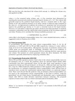
application level, see Figure 1. Such a digital production line provides deep insight into
the materials response and the involved physical effects at each step of the process chain.
Furthermore material parameters can be calculated, which will be used as input data to
perform calculations of subsequently following process steps. In fact, if the production
process chain can be completely reproduced, a backwards approach will be possible, which
allows for the transfer from application requirements to the materials design (computer aided
material design).
A fully theoretical, sufficiently accurate reproduction of all steps of materials processing is -
as far as we know - still not possible. To achieve reliable simulation results in manageable
computational times, (semi-)empirical models are widely used at nearly all production
6
2 Will-be-set-by-IN-TECH
Fig. 1. Continuous full-length models of all production steps from material to application,

exemplarily demonstrating materials design by simulation, e.g. during steel production.
steps. Such models make use of empirically introduced parameters, which must be fitted
to experiments. For example, the description of deformation or fatigue in materials with
complex microstructures, such as in multiphase steels or compound materials (e.g. fiber
reinforced plastics), requires models for various physical effects on a large length- and
timescale. Here, additional to macroscopic finite element analysis on the (centi-)meter scale,
calculations on the microstructure (microscale) down to atomistic models (nanoscale) are
necessary, cf. Figure 2.
To handle the resulting multi-scale problem, different approaches are possible. The classical
approach typically starts at the application level. Here macroscopic calculations are
performed, which may presuppose more detailed investigations. Such details could lead
to smaller length-scales, which mainly result in an increasing number of model-parameters
(input data). On the microstructure level parameters must be taken into account, in particular
to describe morphology and composition as well as the temporal and spatial behaviour of
the microstructures. For instance, for multiphase steels materials data of each phase and
information about its shape and spatial distribution must be known. In case of compound
materials the same arguments hold for the different materials fractions. Moreover, in some
cases an additional description of internal interfaces (e.g. between phases or grains) must be
taken into account, see for example (Artemev et al., 2000; Cahn, 1968; Kobayashi et al., 2000).
By starting from the macro level, all parameters on smaller levels must be available. The
efforts for the measurement of these parameters increase with decreasing length scales.
Therefore, some of the required parameters cannot be measured and must be treated as fitting
parameters or estimated ad hoc.
The ongoing improvement of algorithms and modeling methods accompanying the
continuously rising computer capacities, allow for the use of an alternative approach to
deal with the aforementioned multi-scale problems. Atomistic or even electronic level
calculations can be carried out totally parameter-free (ab-initio calculations) by considering
the interactions between the elemental components of matter. In this context no measurements
are necessary to perform calculations at this level. Experimental data is only used for
validation purposes. By following this theoretical approach, difficult experiments for the

determination of required model parameters on the microscale are supplemented or partially
substituted by adequate calculations. Thus, the need of fitting parameters is drastically
reduced and experimental efforts are minimized, which - in turns - lead to cheaper and faster
development processes.
130
Thermodynamics – Kinetics of Dynamic Systems
Closing the Gap Between Nano- and Macroscale: Atomic Interactions vs. Macroscopic Materials Behavior 3
5m
50
μm
5nm
50 cm
necessary data (input)
calculation time
without details details included
micro -structure
calculation
ab-initio simulation
numerical simulation
Input
experiment
experimentexperiment
Input
experiment
Input
no
Input
“new” simulation approach
“new” simulation approach
classical approach

classical approach
Fig. 2. Modelling on different length scales using different techniques.
However, regardless of the increasing computational capacities, most modern materials -
unfortunately - are still too complex for reliable, purely-theoretical estimations of materials
behaviour. Advanced high-strength steels, in particular, consist of more than 10 components
(e.g. Nb, V, Al, Cr, Mn, etc.) and show different, coexisting lattice structures (e.g., martensite
or austenite), orientations (texture) or precipitates (e.g., carbon nitrides). Moreover, final
properties are often adjusted during advanced materials processing beyond the classical
production line (e.g. annealing during surface galvanizing or hardening during hot stamping
of blanks for automotive light-weight structures).
In order to understand basic mechanisms determining the specific mechanical and
thermodynamic materials characteristics it is necessary to reduce the above-mentioned
complexity. For this reason simple model-systems are considered to study various effects on
the atomistic scale, which crucially determine the macroscopic materials properties. Recent
examples in literature are e.g. binary systems such as Fe-H (Desai et al., 2010; Lee & Jang,
2007; Nazarov et.al., 2010; Psiachos et al., 2011), Fe-C (Hristova et al., 2011; Lee, 2006) or the
eutectic, binary brazing alloy Ag-Cu (Böhme et al., 2007; Feraoun et al., 2001; Najababadi et al,
1993; Williams et al., 2006). Here atomistic methods allow to study the impact of interstitial
elements, mostly without any a-priori assumptions, or to derive required materials data for
microscopic theories (such as phase field studies), which cannot be simply measured by
experiments.
The present work starts with an overview and classification of different interactions models,
beginning with electronic structure theories and ending with empirical atomic potentials. In
order to calculate different thermodynamic and thermo-mechanical materials properties we
consider in Section 3 and 4 the above mentioned alloy Ag-Cu as well as the corresponding
pure components. Two reasons are worth-mentioning for this choice: (a) Ag-Cu is of
high technical relevance and often employed for high-stressed or high-temperature, brazing
connections, e.g. for gas pipe joints. (b) According to the high relevance the materials
behaviour is well-known and a lot of reference data are available; thus all performed
calculations can be easily evaluated. But there is also materials behaviour, which cannot

131
Closing the Gap Between Nano- and Macroscale:
Atomic Interactions vs. Macroscopic Materials Behavior
4 Will-be-set-by-IN-TECH
be directly analyzed by the equations of Sections 3 and 4. In this context mean values
and collective behaviour following from the investigation of many particle systems must be
considered. One possibility for such an analysis is given by molecular dynamics simulations,
which are explained in Section 5. Here we start with a brief description of the basic idea and
framework and then exemplarily present simulations subjected to the temporal evolution of a
misoriented grain in Titanium at finite temperature. The article ends with concluding remarks
and a discussion of future tasks and challenges.
2. Atomic interactions
A central task of atomistic simulation in materials science is to calculate the cohesive energy
for a given set of atoms. The many approaches to achieve this goal differ to a great extent
in accuracy and computational effort. The common aspect, however, is that the calculated
cohesive energy can be utilised to determine a variety of material properties: (i) Differences
in the cohesive energies of stable structures are the basis for determining the relative stability
of different structures or the formation energy of defects and and surfaces. (ii) Differences in
the cohesive energy of metastable and unstable structures are required to calculate e.g. the
energy barriers for diffusion or phase transformation. (iii) Gradients of the cohesive energy
determine the forces acting on the atoms that are needed to carry out structural relaxation
or dynamic simulations. (iv) Derivatives of the cohesive energy are required to calculate e.g.
elastic properties. In the remainder of this section we describe the approaches that span the
regime from highly accurate but computationally expensive electronic-structure calculations
to less accurate but computationally cheap empirical interaction potentials.
2.1 Electronic structure theory
One of the most accurate, yet tractable theoretical approaches in materials science is electronic
structure theory that we will briefly introduce here. For further information we refer the
reader to one of the review papers, e.g. (Bockstedte et al., 1997; Kohn, 1998; Payne et al., 1992),
or textbooks, e.g. (Dreizler & Gross, 1990; Parr & Yang, 1989). The starting point of electronic

structure theory in materials science is the quantum-mechanical description of the material by
the S
CHRÖDINGER equation
1
(

H
− E)Ψ =(

T
e
+

T
i
+

V
e−e
+

V
e−i
+

V
i−i
− E)Ψ = 0. (1)
for ions (i.e. the atomic nuclei) and electrons with a many-body wavefunction Ψ.The
terms


V
e−e
,

V
e−i
and

V
i−i
describe the COULOMB interactions between electrons/electrons,
electrons/ions, as well as ions/ions. The terms

T
e
and

T
i
denote the kinetic energies of
the electrons and ions. The structure and properties of many-body systems can then be
determined by solving the S
CHRÖDINGER equation. Most practical applications simplify
this matter by assuming a decoupled movement of electrons and ions (B
ORN-OPPENHEIMER
approximation (Born & Oppenheimer, 1927)) and thereby reducing the problem to the
interaction of the electrons among each other. This interaction is determined by the C
OULOMB
1

Without loss of generality we refer through the work to Cartesian coordinates. Scalar quantities are
written in italic letters (s); vectors are single underlined (v
); tensors or matrices of second or higher
order are double underlined (T
) or marked by blackboard capital letters (M). Operators are indicated
by the
()-symbol. Scalar products between vectors and tensors are marked with (·)or(··), respectively.
Greek indices refer to atoms (αβγ)orelectrons(μνξ).
132
Thermodynamics – Kinetics of Dynamic Systems
Closing the Gap Between Nano- and Macroscale: Atomic Interactions vs. Macroscopic Materials Behavior 5
potential and the PAULI principle. There are several approaches to solve the remaining
quantum-mechanical problem, the most successful one being density-functional theory that
can be considered the today standard method of calculating material properties accurately.
2.2 Density-functional theory
Density-functional theory originates from the KOHN-SHAM formalism (Hohenberg & Kohn,
1964; Kohn & Sham, 1965) that is based on the electron density ρ of a system which describes
the number of electrons per unit volume:
ρ
(r
1
)=N



|Ψ(x
1
, , x
N
)|

2
dx
2
dx
N
.(2)
The volume-integral of this quantity is the total number of electrons

ρ(r) dr = N (3)
in the system. K
OHN and SHAM mapped the problem of a system of N interacting electrons
onto the problem of a set of systems of non-interacting electrons in the effective potential v
eff
of the other electrons. The SCHRÖDINGER equation for electrons in the non-interacting system
is then

−
1
2
∇
2
+ v
eff
(r)

ψ
n
(r)=ε
n
ψ

n
(r) , n = 1 N (4)
with the electronic density of N electrons of spin s
ρ
(r)=
N
∑
n=1
∑
s
|ψ
n
(r , s)|
2
.(5)
The effective potential v
eff
v
eff
(r)=v( r)+v
H
(r)+v
xc
(r) ,(6)
includes the Hartree-potential v
H
and the so-called exchange-correlation energy functional
v
xc
(r) that is not known a priori and that needs to be approximated. The most widely

used approximations to the exchange-correlation functional are the local-density approximation
(LDA) and the generalized-gradient approximation (GGA).
2.3 Tight-binding and bond-order potentials
The limitation of DFT to small systems (few 100 atoms) due to the numerical cost can be
overcome by taking the description of the electronic structure to an approximate level. This
can be carried out rigorously by approximating the density functional theory (DFT) formalism
in terms of physically and chemically intuitive contributions within the tight-binding (TB)
bond model (Sutton et al., 1988). The TB approximation is sufficiently accurate to predict
structural trends as well as sufficiently intuitive for a physically meaningful interpretation
of the bonding. The tight-binding model is a coarse-grained description of the electronic
structure that expresses the eigenfunctions ψ
n
of the KOHN-SHAM equation in a minimal basis
ψ
n
=
∑
αμ
c
(n)
αμ
αμ (7)
133
Closing the Gap Between Nano- and Macroscale:
Atomic Interactions vs. Macroscopic Materials Behavior