Two Phase Flow Phase Change and Numerical Modeling Part 5 pptx
Bạn đang xem bản rút gọn của tài liệu. Xem và tải ngay bản đầy đủ của tài liệu tại đây (676.86 KB, 30 trang )
Two Phase Flow, Phase Change and Numerical Modeling
110
Fig. 14. Evolution of the curvature radius along a microchannel
In the evaporator and adiabatic zones, the curvature radius, in the parallel direction of the
microchannel axis, is lower than the one perpendicular to this axis. Therefore, the meniscus
is described by only one curvature radius. In a given section, r
c
is supposed constant. The
axial evolution of r
c
is obtained by the differential of the Laplace-Young equation. The part
of wall that is not in contact with the liquid is supposed dry and adiabatic.
In the condenser, the liquid flows toward the microchannel corners. There is a transverse
pressure gradient, and a transverse curvature radius variation of the meniscus. The
distribution of the liquid along a microchannel is presented in Fig. 14.
The microchannel is divided into several elementary volumes of length, dz, for which, we
consider the Laplace-Young equation, and the conservation equations written for the liquid
and vapor phases as it follows
Laplace-Young equation
vl c
2
c
dP dP dr
dz dz r dz
σ
−=− (9)
Liquid and vapor mass conservation
()
lll
v
d w A
1dQ
dz h dz
ρ
=
Δ
(10)
()
vvv
v
d w A
1dQ
-
dz h dz
ρ
=
Δ
(11)
Liquid and vapor momentum conservation
2
ll ll
lilillwlwll
d(A w ) d(A P )
dz dz A A
g
Asin dz
dz dz
ρ=+τ+τ−ρβ
(12)
Theoretical and Experimental Analysis of Flows and Heat Transfer
within Flat Mini Heat Pipe Including Grooved Capillary Structures
111
2
vv vv
vililvwvwvv
d(A w ) d(A P )
dz dz A A
g
Asin dz
dz dz
ρ=−−τ−τ−ρβ (13)
Energy conservation
()
2
w
wwsat
2
ww
Th 1dQ
TT
zt ltdz
∂
λ−−=−
∂×
(14)
The quantity dQ/dz in equations (10), (11), and (14) represents the heat flux rate variations
along the elementary volume in the evaporator and condenser zones, which affect the
variations of the liquid and vapor mass flow rates as it is indicated by equations (10) and
(11). So, if the axial heat flux rate distribution along the microchannel is given by
ae e
aeea
ea
aeatb
cb
Q z/L 0 z L
Q Q L z L L
LL - z
Q 1 L L z L L
L - L
≤≤
=<<+
+
++≤≤−
(15)
we get a linear flow mass rate variations along the microchannel.
In equation (15), h represents the heat transfer coefficient in the evaporator, adiabatic and
condenser sections. For these zones, the heat transfer coefficients are determined from the
experimental results (section 5.3.3). Since the heat transfer in the adiabatic section is equal to
zero and the temperature distribution must be represented by a mathematical continuous
function between the different zones, the adiabatic heat transfer coefficient value is chosen
to be infinity.
The liquid and vapor passage sections, A
l
, and A
v
, the interfacial area, A
il
, the contact areas
of the phases with the wall, A
lp
and A
vp
, are expressed using the contact angle and the
interface curvature radius by
22
lc
sin 2
A 4rsin
2
θ
=∗ θ−θ+
(16)
2
vl
AdA=− (17)
il c
A8 rdz=×θ×× (18)
lw c
16
Arsin dz
2
=θ
(19)
vw c
16
A4d-rsin dz
2
=× θ
(20)
4
π
θ= −α
(21)
Two Phase Flow, Phase Change and Numerical Modeling
112
The liquid-wall and the vapor-wall shear stresses are expressed as
2
lw l l l
1
wf
2
τ=ρ
,
l
l
l
e
k
f
R
= ,
llhlw
el
l
wD
R
ρ
=
μ
(22)
2
vw v v v
1
wf
2
τ=ρ
,
v
v
ev
k
f
R
= ,
vvhvw
ev
v
wD
R
ρ
=
μ
(23)
Where k
l
and k
v
are the Poiseuille numbers, and D
hlw
and D
hvw
are the liquid-wall and the
vapor-wall hydraulic diameters, respectively.
The hydraulic diameters and the shear stresses in equations (22) and (23) are expressed as
follows
2
c
hlw
sin 2
2rsin
2
D
sin
θ
×θ−θ+
=
θ
(24)
222
c
hvw
c
sin 2
d4rsin
2
D
4
dsinθ r
2
θ
−θ−θ+
=
−×
(25)
lll
lw
2
c
1kwsin
sin
2
22sin r
2
μθ
τ=
θ
θ−θ+
(26)
vvv c
vw
222
c
4
kw d sin r
2
sin
2d 4r sin
2
μ− θ
τ=
θ
−θ−θ+
(27)
The liquid-vapor shear stress is calculated by assuming that the liquid is immobile since its
velocity is considered to be negligible when compared to the vapor velocity (w
l
<< w
v
).
Hence, we have
2
vvv
il
eiv
1wk
2R
ρ
τ= ,
v v hiv
eiv
v
wD
R
ρ
=
μ
(28)
where D
hiv
is the hydraulic diameter of the liquid-vapor interface. The expressions of D
hiv
and τ
iv
are
222
c
hi
c
sin 2
d4rsin
2
D
2r
θ
−θ−θ+
=
θ
(29)
vcvv
il
222
c
krw
sin 2
d4rsin
2
θμ
τ=
θ
−θ−θ+
(30)
Theoretical and Experimental Analysis of Flows and Heat Transfer
within Flat Mini Heat Pipe Including Grooved Capillary Structures
113
The equations (9-14) constitute a system of six first order differential, nonlinear, and coupled
equations. The six unknown parameters are: r
c
, w
l
, w
v
, P
l
, P
v
, and T
w
. The integration starts
in the beginning of the evaporator (z = 0) and ends in the condenser extremity (z = L
t
- L
b
),
where L
b
is the length of the condenser flooding zone. The boundary conditions for the
adiabatic zone are the calculated solutions for the evaporator end. In z = 0, we use the
following boundary conditions:
()
0
ccmin
00
lv
0
vsatv
0
lv
cmin
r r (a)
w w 0 (b)
P P T (c)
P P - (d)
r
=
==
=
σ
=
(31)
The solution is performed along the microchannel if r
c
is higher than r
cmin
. The coordinate
for which this condition is verified, is noted L
as
and corresponds to the microchannel dry
zone length. Beyond this zone, the liquid doesn't flow anymore. Solution is stopped when r
c
= r
cmax
, which is determined using the following reasoning: the liquid film meets the wall
with a constant contact angle. Thus, the curvature radius increases as we progress toward
the condenser (Figs. 14a and 14b). When the liquid film contact points meet, the wall is not
anymore in direct contact with vapor. In this case, the liquid configuration should
correspond to Fig. 14c, but actually, the continuity in the liquid-vapor interface shape
imposes the profile represented on Figure 14d. In this case, the curvature radius is
maximum. Then, in the condenser, the meniscus curvature radius decreases as the liquid
thickness increases (Fig. 14e). The transferred maximum power, so called capillary limit, is
determined if the junction of the four meniscuses starts precisely in the beginning of the
condenser.
6.2 Numerical results and analysis
In this analysis, we study a FMHP with the dimensions which are indicated in Table 1. The
capillary structure is composed of microchannels as it is represented by the sketch of Fig. 1.
The working fluid is water and the heat sink temperature is equal to 40 °C. The conditions of
simulation are such as the dissipated power is varied, and the introduced mass of water is
equal to the optimal fill charge.
The variations of the curvature radius r
c
are represented in Fig. 15. In the evaporator,
because of the recession of the meniscus in the channel corners and the great difference of
pressure between the two phases, the interfacial curvature radius is very small on the
evaporator extremity. It is also noticed that the interfacial curvature radius decreases in the
evaporator section when the heat flux rate increases. However, it increases in the condenser
section. Indeed, when the heat input power increases, the liquid and vapor pressure losses
increase, and the capillary pressure becomes insufficient to overcome the pressure losses.
Hence, the evaporator becomes starved of liquid, and the condenser is blocked with the
liquid in excess.
The evolution of the liquid and vapor pressures along the microchannel is given in Figs. 16
and 17. We note that the vapor pressure gradient along the microchannel is weak. It is due
to the size and the shape of the microchannel that don't generate a very important vapor
Two Phase Flow, Phase Change and Numerical Modeling
114
pressure drop. For the liquid, the velocity increase is important near of the evaporator
extremity, which generates an important liquid pressure drop.
Fig. 18 presents the evolution of the liquid phase velocity along a microchannel. In the
evaporator section, as the liquid passage section decreases, the liquid velocity increases
considerably. On other hand, since the liquid passage section increases along the
microchannel (adiabatic and condenser sections), the liquid velocity decreases to reach zero
at the final extremity of the condenser. In the evaporator, the vapor phase velocity increases
since the vapor passage section decreases. In the adiabatic zone, it continues to grow with
the reduction of the section of vapor passage. Then, when the condensation appears, it
decreases, and it is equal to zero on the extremity of the condenser (Fig. 19).
1.00E-04
1.10E-04
1.20E-04
1.30E-04
1.40E-04
1.50E-04
1.60E-04
1.70E-04
1.80E-04
0 0.010.020.030.040.050.060.070.080.09 0.1
z (m)
r
c
(m)
10 W
20 W
30 W
40 W
50 W
60 W
10 W
20 W
30 W
40 W
50 W
60 W
Evaporator Adiabatic Zone Condenser
Fig. 15. Variations of the curvature radius r
c
of the meniscus
8.00E-05
5.00E+03
1.00E+04
1.50E+04
2.00E+04
2.50E+04
3.00E+04
3.50E+04
0 0.01 0.02 0.03 0.04 0.05 0.06 0.07 0.08 0.09 0.1
z (m)
P
v
(Pa)
Evaporator Adiabatic Zone Condenser
10 W
20 W
30 W
40 W
50 W
60 W
Fig. 16. Variations of the vapor pressure P
v
Theoretical and Experimental Analysis of Flows and Heat Transfer
within Flat Mini Heat Pipe Including Grooved Capillary Structures
115
8.00E-05
5.00E+03
1.00E+04
1.50E+04
2.00E+04
2.50E+04
3.00E+04
0 0.01 0.02 0.03 0.04 0.05 0.06 0.07 0.08 0.09 0.1
z (m)
P
l
(Pa)
Evaporator Adiabatic Zone Condenser
10 W
20 W
30 W
40 W
50 W
60 W
Fig. 17. Variations of the liquid pressure P
l
8.00E-05
5.08E-03
1.01E-02
1.51E-02
2.01E-02
2.51E-02
0 0.01 0.02 0.03 0.04 0.05 0.06 0.07 0.08 0.09 0.1
z (m)
w
l
(m/s)
Evaporator Adiabatic Zone Condenser
10 W
20 W
30 W
40 W
50 W
60 W
Fig. 18. The liquid phase velocity distribution
0.0
0.5
1.0
1.5
2.0
2.5
3.0
3.5
0 0.01 0.02 0.03 0.04 0.05 0.06 0.07 0.08 0.09 0.1
z (m)
w
v
(m/s)
10 W
20 W
30 W
40 W
50 W
60 W
Evaporator
Adiabatic Zone
Condenser
Fig. 19. The vapor phase velocity distribution
Two Phase Flow, Phase Change and Numerical Modeling
116
The variations of the wall temperature along the microchannel are reported in Fig. 20. In the
evaporator section, the wall temperature decreases since an intensive evaporation appears
due the presence of a thin liquid film in the corners. In the adiabatic section, the wall
temperature is equal to the saturation temperature corresponding to the vapor pressure. In
the condenser section, the wall temperature decreases. In this plot, are shown a comparison
between the numerical results and the experimental ones, and a good agreement is found
between the temperature distribution along the FMHP computed from the model and the
temperature profile which is measured experimentally. An agreement is also noticed
between the temperature distribution which is obtained from a pure conduction model and
that obtained experimentally (Fig. 21).
20
30
40
50
60
70
80
90
100
110
0 0.01 0.02 0.03 0.04 0.05 0.06 0.07 0.08 0.09 0.1
z (mm)
T (°C)
Experimental 10 W
Experimental 20 W
Experimental 30 W
Experimental 40 W
Experimental 50 W
Experimental 60 W
Model
Evaporator
Adiabatic zone Condenser
Fig. 20. Variations of the FMHP wall temperature
0
20
40
60
80
100
120
140
160
180
0 0.01 0.02 0.03 0.04 0.05 0.06 0.07 0.08 0.09 0.1
z (mm)
T (°C)
Experimental 10 W
Experimental 20 W
Experimental 30 W
Experimental 40 W
Experimental 50 W
Experimental 60 W
Model
Fig. 21. Variations of the copper plate wall temperature
7. Conclusion
In this study, a copper FMHP is machined, sealed and filled with water as working fluid.
The temperature measurements allow for a determination of the temperature gradients and
maximum localized temperatures for the FMHPs. The thermal FMHP are compared to those
Theoretical and Experimental Analysis of Flows and Heat Transfer
within Flat Mini Heat Pipe Including Grooved Capillary Structures
117
of a copper plate having the same dimensions. In this way, the magnitude of the thermal
enhancement resulting from the FMHP could be determined. The thermal measurements
show significantly reduced temperature gradients and maximum temperature decrease
when compared to those of a copper plate having the same dimensions. Reductions in the
source-sink temperature difference are significant and increases in the effective thermal
conductivity of approximately 250 percent are measured when the flat mini heat pipes
operate horizontally.
The main feature of this study is the establishment of heat transfer laws for both
condensation and evaporation phenomena. Appropriate dimensionless numbers are
introduced and allow for the determination of relations, which represent well the
experimental results. This kind of relations will be useful for the establishment of theoretical
models for such capillary structures.
Based on the mass conservation, momentum conservation, energy conservation, and
Laplace-Young equations, a one dimensional numerical model is developed to simulate the
liquid-vapor flow as well as the heat transfer in a FMHP constituted by microchannels. It
allows to predict the maximum power and the optimal mass of the fluid. The model takes
into account interfacial effects, the interfacial radius of curvature, and the heat transfer in
both the evaporator and condenser zones. The resulting coupled ordinary differential
equations are solved numerically to yield interfacial radius of curvature, pressure, velocity,
temperature information as a function of axial distance along the FMHP, for different heat
inputs. The model results predict an almost linear profile in the interfacial radius of
curvature. The pressure drop in the liquid is also found to be about an order of magnitude
larger than that of the vapor. The model predicts very well the temperature distribution
along the FMHP.
Although not addressing several issues such as the effect of the fill charge, FMHP
orientation, heat sink temperature, and the geometrical parameters (groove width, groove
height or groove spacing), it is clear from these results that incorporating such FMHP as
part of high integrated electronic packages can significantly improve the performance and
reliability of electronic devices, by increasing the effective thermal conductivity,
decreasing the temperature gradients and reducing the intensity and the number of
localized hot spots.
8. References
Angelov, G., Tzanova, S., Avenas, Y., Ivanova, M., Takov, T., Schaeffer, C. & Kamenova, L.
(2005). Modeling of Heat Spreaders for Cooling Power and Mobile Electronic
Devices,
36
th
Power Electronics Specialists Conference (PESC 2005), pp. 1080-1086,
Recife, Brazil, June 12-15, 2005
Avenas, Y., Mallet, B., Gillot, C., Bricard, A., Schaeffer, C., Poupon, G. & Fournier, E. (2001).
Thermal Spreaders for High Heat Flux Power Devices,
7
th
THERMINIC Workshop,
pp. 59-63, Paris, France, September 24-27, 2001
Cao, Y., Gao, M., Beam, J.E. & Donovan, B. (1997). Experiments and Analyses of Flat
Miniature Heat Pipes,
Journal of Thermophysics and Heat Transfer, Vol.11, No.2, pp.
158-164
Cao, Y. & Gao, M. (2002). Wickless Network Heat Pipes for High Heat Flux Spreading
Applications,
International Journal of Heat and Mass Transfer, Vol.45, pp. 2539-2547
Two Phase Flow, Phase Change and Numerical Modeling
118
Chien, H.T., Lee, D.S., Ding, P.P., Chiu, S.L. & Chen, P.H. (2003). Disk-shaped Miniature
Heat Pipe (DMHP) with Radiating Micro Grooves for a TO Can Laser Diode
Package,
IEEE Transactions on Components and Packaging Technologies, Vol.26, No.3,
pp. 569-574
Do, K.H., Kim, S.J. & Garimella, S.V. (2008). A Mathematical Model for Analyzing the
Thermal Characteristics of a Flat Micro Heat Pipe with a Grooved Wick,
International Journal Heat and Mass Transfer, Vol.51, No.19-20, pp. 4637-4650
Do, K.H. & Jang, S.P. (2010). Effect of Nanofluids on the Thermal Performance of a Flat
Micro Heat Pipe with a Rectangular Grooved Wick,
International Journal of Heat and
Mass Transfer
, Vol.53, pp. 2183-2192
Gao, M. & Cao, Y. (2003). Flat and U-shaped Heat Spreaders for High-Power Electronics,
Heat Transfer Engineering, Vol.24, pp. 57-65
Groll, M., Schneider, M., Sartre, V., Zaghdoudi, M.C. & Lallemand, M. (1998). Thermal
Control of electronic equipment by heat pipes,
Revue Générale de Thermique, Vol.37,
No.5, pp. 323-352
Hopkins, R., Faghri, A. & Khrustalev, D. (1999). Flat Miniature Heat Pipes with Micro
Capillary Grooves,
Journal of Heat Transfer, Vol.121, pp. 102-109
Khrustlev, D. & Faghri, A. (1995). Thermal Characteristics of Conventional and Flat
Miniature Axially Grooved Heat Pipes,
Journal of Heat Transfer, Vol.117, pp. 1048-
1054
Faghri, A. & Khrustalev, D. (1997). Advances in modeling of enhanced flat miniature heat
pipes with capillary grooves, Journal of Enhanced Heat Transfer, Vol.4, No.2, pp.
99-109
Khrustlev, D. & Faghri, A. (1999). Coupled Liquid and Vapor Flow in Miniature Passages
with Micro Grooves,
Journal of Heat Transfer, Vol.121, pp. 729-733
Launay, S., Sartre, V. & Lallemand, M. (2004). Hydrodynamic and Thermal Study of a
Water-Filled Micro Heat Pipe Array,
Journal of Thermophysics and Heat Transfer,
Vol.18, No.3, pp. 358-363
Lefèvre, F., Revellin, R. & Lallemand, M. (2003). Theoretical Analysis of Two-Phase Heat
Spreaders with Different Cross-section Micro Grooves,
7th International Heat Pipe
Symposium
, pp. 97-102, Jeju Island, South Korea, October 12-16, 2003
Lefèvre, F., Rullière, R., Pandraud, G. & Lallemand, M. (2008). Prediction of the Maximum
Heat Transfer Capability of Two-Phase Heat Spreaders-Experimental Validation,
International Journal of Heat and Mass Transfer, Vol.51, No.15-16, pp. 4083-4094
Lim, H.T., Kim, S.H., Im, H.D., Oh, K.H. & Jeong, S.H. (2008). Fabrication and Evaluation of
a Copper Flat Micro Heat Pipe Working under Adverse-Gravity Orientation,
Journal of Micromechanical Microengineering, Vol.18, 8p.
Lin, L., Ponnappan, R. & Leland, J. (2002). High Performance Miniature Heat Pipe,
International Journal of Heat and Mass Transfer, Vol.45, pp. 3131-3142
Lin, J.C., Wu, J.C., Yeh, C.T. & Yang, C.Y. (2004). Fabrication and Performance Analysis of
Metallic Micro Heat Spreader for CPU,
13
th
International Heat Pipe Conference, pp.
151-155, Shangai, China, September 21-25, 2004
Moon, S.H., Hwang, G., Ko, S.C. & Kim, Y.T. (2003). Operating Performance of Micro Heat
Pipe for Thin Electronic Packaging,
7
th
International Heat Pipe Symposium, pp. 109-
114, Jeju Island, South Korea, October 12-16, 2003
Theoretical and Experimental Analysis of Flows and Heat Transfer
within Flat Mini Heat Pipe Including Grooved Capillary Structures
119
Moon, S.H., Hwang, G., Ko, S.C. & Kim, Y.T. (2004). Experimental Study on the Thermal
Performance of Micro-Heat Pipe with Cross-section of Polygon,
Microelectronics
Reliability
, Vol.44, pp. 315-321
Murakami, M., Ogushi, T., Sakurai, Y., Masumuto, H., Furukawa, M. & Imai, R. (1987). Heat
Pipe Heat Sink,
6
th
International Heat Pipe Conference, pp. 257-261, Grenoble, France,
May 25-29, 1987
Ogushi, T. & Yamanaka, G. (1994). Heat Transport Capability of Grooves Heat Pipes,
5
th
International Heat Pipe Conference
, pp. 74-79, Tsukuba, Japan, May 14-18, 1994
Plesh, D., Bier, W. & Seidel, D. (1991). Miniature Heat Pipes for Heat Removal from
Microelectronic Circuits,
Micromechanical Sensors, Actuators and Systems, Vol.32, pp.
303-313
Popova, N., Schaeffer, C., Sarno, C., Parbaud, S. & Kapelski, G. (2005). Thermal management
for stacked 3D microelectronic packages,
36th Annual IEEE Power Electronic
Specialits Conference (PESC 2005)
, pp. 1761-1766, recife, Brazil, June 12-16, 2005
Popova, N., Schaeffer, C., Avenas, Y. & Kapelski, G. (2006). Fabrication and Experimental
Investigation of Innovative Sintered Very Thin Copper Heat Pipes for Electronics
Applications,
37th IEEE Power Electronics Specialist Conference (PESC 2006), pp. 1652-
1656, Vol. 1-7, Cheju Island, South Korea, June 18-22, 2006
Romestant, C., Burban, G. & Alexandre, A. (2004). Heat Pipe Application in Thermal-Engine
Car Air Conditioning,
13
th
International Heat Pipe Conference, pp. 196-201, Shanghai,
China, September 21-25, 2004
Schneider, M., Yoshida, M. & Groll, M. (1999a). Investigation of Interconnected Mini Heat
Pipe Arrays For Micro Electronics Cooling,
11
th
International Heat Pipe conference,
6p., Musachinoshi-Tokyo, Japan, September 12-16, 1999
Schneider, M. Yoshida, M. & Groll, M. (1999b). Optical Investigation of Mini Heat Pipe
Arrays With Sharp Angled Triangular Grooves,
Advances in Electronic Packaging,
EEP-Vol. 26-1 and 26-2, 1999, pp. 1965-1969.
Schneider, M. Yoshida, M. & Groll, M. (2000). Cooling of Electronic Components By Mini
Heat Pipe Arrays,
15
th
National Heat and Mass transfer Conference and 4
th
ISHMT/ASME Heat and Mass Transfer Conference, 8p., Pune, India, January 12-14,
2000
Soo Yong, P. & Joon Hong, B. (2003). Thermal Performance of a Grooved Flat-Strip Heat
Pipe with Multiple Source Locations,
7
th
International Heat Pipe Symposium, pp. 157-
162, Jeju Island, South Korea, October 12-16, 2003
Shi, P.Z., Chua, K.M., Wong, S.C.K. & Tan, Y.M. (2006). Design and Performance
Optimization of Miniature Heat Pipe in LTCC,
Journal of Physics: Conference Series,
Vol.34, pp. 142-147
Sun, J.Y. & Wang, C.Y. (1994). The Development of Flat Heat Pipes for Electronic Cooling,
4
th
International Heat Pipe Symposium, pp. 99-105, Tsukuba, Japan, May 16-18, 1994
Tao, H.Z., Zhang, H., Zhuang, J. & Bowmans, J.W. (2008). Experimental Study of Partially
Flattened Axial Grooved Heat Pipes,
Applied Thermal Engineering, Vol.28, pp. 1699-
1710
Tzanova, S., Ivanova, M., Avenas, Y. & Schaeffer, C. (2004). Analytical Investigation of Flat
Silicon Micro Heat Spreaders,
Industry Applications Conference, 39
th
IAS Annual
Meeting Conference Record of the 2004 IEEE, pp. 2296-2302, Vol.4, October 3-7, 2004
Two Phase Flow, Phase Change and Numerical Modeling
120
Xiaowu, W., Yong, T. & Ping, C. (2009). Investigation into Performance of a Heat Pipe with
Micro Grooves Fabricated by Extrusion-Ploughing Process,
Energy Conversion and
Management
, Vol.50, pp.1384-1388
Zaghdoudi, M.C. & Sarno, C. (2001). Investigation on the Effects of Body Force Environment
on Flat Heat Pipes,
Journal of Thermophysics and Heat Transfer, Vol.15, No.4, pp. 384-
394
Zaghdoudi, M.C., Tantolin, C. & Godet, C. (2004). Experimental and Theoretical Analysis of
Enhanced Flat Miniature Heat Pipes,
Journal of Thermophysics and Heat Transfer,
Vol.18, No.4, pp. 430-447
Zhang, L., Ma, T., Zhang, Z.F. & Ge, X. (2004). Experimental Investigation on Thermal
Performance of Flat Miniature Heat Pipes with Axial Grooves,
13
th
International
Heat Pipe Conference
, pp. 206-210, Shangai, China, September 21-25, 2004
Zhang, M., Liu, Z. & Ma, G. (2009). The Experimental and Numerical Investigation of a
Grooved Vapor Chamber,
Applied Thermal Engineering, Vol.29, pp. 422-430
6
Modeling Solidification Phenomena in the
Continuous Casting of Carbon Steels
Panagiotis Sismanis
SIDENOR SA
Greece
1. Introduction
In recent years the quest for advanced steel quality satisfying more stringent specifications
by time has forced research in the development of advanced equipment for the
improvement of the internal structure of the continuously cast steels. A relatively important
role has played the better understanding of the solidification phenomena that occur during
the final stages of the solidification. Dynamic soft-reduction machines have been placed in
industrial practice with top-level performance. Nevertheless, the numerical solution of the
governing heat-transfer differential equation under the proper initial and boundary
conditions continues to play the paramount role for the fundamental approach of the whole
solidification process. Steel properties are critical upon the solidification behaviour.
Different chemical analyses of carbon steels alter the solidus and liquidus temperatures and
therefore influence the calculated results. Shell growth, local cooling rates and solidification
times, solid fraction, and secondary dendrite arm-spacing are some important metallurgical
parameters that need to be ultimately computed for specific steel grades once the heat
transfer problem is solved.
2. Previous work and current status
Solidification heat-transfer has been extensively studied throughout the years and there are
numerous works on the subject in the academic and industrial fields. Towards the
development of continuous casting machines adapted to the needs of the various steel
grades a great deal of research work has been published in this metallurgical domain. In one
of the early works (Mizikar, 1967), the fundamental relationships and the means of solution
were described, but in a series of articles (Brimacombe, 1976) and (Brimacombe et al, 1977,
1978, 1979, 1980) some important answers to the heat transfer problem as well as to
associated product internal structures and continuous-casting problems were presented in
detail. The crucial knowledge-creation practice of combining experiments and models
together was the main method applied to most of these works. In this way, the shell
thickness at mold exit, the metallurgical length of the caster, the location down the caster
where cracks initiate, and the cooling practice below the mold to avoid reheating cracks
were some of the points addressed. At that time, the first finite-element thermal-stress
models of solidification were applied in order to understand the internal stress distribution
in the solidifying steel strand below the mold. The need for data with respect to the
Two Phase Flow, Phase Change and Numerical Modeling
122
mechanical properties of steels and specifically creep at high temperatures as a means for
controlling the continuous casting events was realized from the early years of analysis
(Palmaers, 1978). In a similar study, the bulging produced by creep in the continuously cast
slabs was analyzed (Grill & Schwerdtfeger, 1979) with a finite-element model. In order to
simulate the unbending process in a continuous casting machine a multi-beam model was
proposed (Tacke, 1985) for strand straightening in the caster. With the advent of the
computer revolution more advanced topics relevant to the fluid flow in the mold were
addressed. Unsteady-state turbulent phenomena in the mold were tackled using the large
eddy simulation method of analysis (Sivaramakrishnan et al, 2000); in extreme cases, it was
reported that the computer program could take up to a month to converge and come up
with a solution. Nevertheless, computational heat-transfer programs have helped in the
development of better internal structure continuously-cast steels mostly for two main
reasons: [1] the online control of the casting process and, [2] the offline analysis of factors
which are more intrinsic to the specific nature of a steel grade under investigation, i.e.,
chemical analysis and internal structure. Continuing the literature survey more focus will be
given to selected published works relevant to the second [2] influential reason.
The formation of internal cracks that influence the internal structure of slabs was
investigated from the early years (Fuji et al, 1976) of continuous casting. It was proven that
internal cracks are formed adjacent to the solid-liquid interface and greatly influenced by
bulging. As creep was critical upon bulging in continuously cast slabs a model was
proposed (Fujii et al, 1981) with adequate agreement between theory and practice for low
and medium carbon aluminum-killed steels. In another study (Matsumiya et al, 1984) a
mathematical analysis model was established in order to investigate the interdendritic
micro-segregation using a finite difference scheme and taking into consideration the
diffusion of a solute in the solid and liquid phases. As mechanical behavior of plain carbon
steel in the austenite temperature region was proven of paramount importance in the
continuous casting process a set of simple constitutive equations was developed (Kozlowski
et al, 1992) for the elastoplastic analysis used in finite element models. Chemical
composition of steel and specifically equivalent carbon content as well as the Mn/S ratio
were found to define a critical strain value above which internal structure problems could
appear (Hiebler et al, 1994). As analysis deepened into the internal structure and specifically
into micro- and macro-segregation, relationships between primary and secondary dendrite
arm spacing (Imagumbai, 1994) started to appear. In fact, first order analysis revealed that
secondary dendrite arm-spacing is about one-half of the primary one. The effect of cooling
rate on zero-strength-temperature (ZST) and zero-ductility-temperature (ZDT) was found to
be significant (Won et al, 1998) due to segregation of solute elements at the final stage of
solidification. The calculated temperatures at the solid fractions of 0.75 and 0.99
corresponded to the experimentally measured ZST and ZDT, respectively. Furthermore, a
set of relationships that take under consideration steel composition, cooling rate, and solid
fraction was proposed; the suggested prediction equation on ZST and ZDT was found in
relative agreement with experimental results. In a monumental work (Cabrera-Marrero et al,
1998), the dendritic microstructure of continuously-cast steel billets was analyzed and found
in agreement with experimental results. In fact, the differential equation of heat transfer was
numerically solved along the sections of the caster and local solidification times related to
microstructure for various steel compositions were computed. Based on the Clyne-Kurz
model a simple model of micro-segregation during solidification of steels was developed
Modeling Solidification Phenomena in the Continuous Casting of Carbon Steels
123
(Won & Thomas, 2001). In this way, the secondary dendrite arm spacing can be sufficiently
computed with respect to carbon content and local cooling rates. In another study (Han et al,
2001), the formation of internal cracks in continuously cast slabs was mathematically
analyzed with the implementation of a strain analysis model together with a micro-
segregation model. The equation of heat transfer was also numerically solved along the
caster. Total strain based on bulging, unbending, and roll-misalignment attributed strains,
was computed and checked against the critical strain. Consequently, internal structure
problems could be identified and verified in practice. The unsteady bulging was found to be
(Yoon et al, 2002) the main reason of mold level hunching during thin slab casting. A finite
difference scheme for the numerical solution of the heat transfer equation together with a
continuous beam model and a primary creep equation were developed in order to match
experimental data. A 2D unsteady heat-transfer model (Zhu et al, 2003) was applied to
obtain the surface temperature and shell thickness of continuous casting slabs during the
process of solidification. Roll misalignment was proven to provoke internal cracks once total
strain at the solid/liquid interface exceeded the critical strain for the examined chemical
composition of steel slabs. As creep was proven to be important in the continuous casting of
steels, an evaluation of common constitutive equations was performed (Pierer at al, 2005)
and tested against experimental data. The proposed results could help in the development
of more sophisticated 2D finite element models. Once offline computer models are proven
correct they can be applied online in real-time applications and minimize internal defects
(Ma et al, 2008).
Consequently, very advanced types of continuous casting machines have appeared in the
international market as a result of these investigations. Different steel grades are classified
into groups which are processed in the continuous casters as heats cast with similar design
and operating parameters. Automation plays an important role supervising the whole
continuous casting process by running in two levels, i.e., controlling the process, and
computing the final solidification front as a real-time solution to the heat-transfer problem
case. The numerous steel products of excellent quality manifest the success of these
sophisticated casting machines.
3. Present work
In this work the modelling of the solidification phenomena for two slab casters installed in
different plants, one in Stomana, Pernik, Bulgaria, and the other in Sovel, Almyros, Greece,
is presented. Both plants belong to the SIDENOR group of companies. Simple design and
operating parameters together with the chemical analyses of the steel grades cast are the
basic data to approximate the heat transfer solution, compute the temperature distributions
inside the continuously cast slabs in every section of the caster, and investigate the
solidification phenomena from the metallurgical point of view. A 3D numerical solution of
the differential equation of heat transfer was developed and tested in a previous publication
(Sismanis, 2010) and is not to be presented in detail here. Some routines were also
implemented in the main core of that developed software in order to cover the extra
computational work required for the metallurgical analysis of the solidification phenomena.
Furthermore, strain analysis for any slab bulging and for the straightening positions was
implemented as well. The methodology applied for tackling the continuous casting
problem for different carbon steel grades from the metallurgical point of view is maybe
Two Phase Flow, Phase Change and Numerical Modeling
124
what makes this purely computational study more intriguing and specific in nature. Critical
formulas that bind the heat transfer problem with the various solidification parameters and
strains in the slab are presented and discussed.
3.1 The heat transfer model applied
The general 3D heat transfer equation that describes the temperature distribution inside the
solidifying body is given by the following equation (Carslaw & Jaeger, 1986) and (Incropera
& DeWitt, 1981):
P
T
CkTS
t
ρ
∂
=∇⋅ ∇ +
∂
(1)
The source term S, in units W· m
-3
, may be considered (Patankar, 1980) to be of the form:
CP
SS ST=+⋅ (2)
that is, by a constant term and a temperature dependent term and can be related to
correspond to the latent heat of phase change. Furthermore, T is the temperature, and ρ, C
p
,
and k are the density, heat capacity, and thermal conductivity of steel, respectively. The heat
transfer equation in Cartesian coordinates may be written as:
p
TT T T
CkkkS
txx yy zz
ρ
∂∂∂ ∂∂ ∂∂
=+++
∂∂ ∂ ∂ ∂ ∂ ∂
(3)
The solidification problem in the continuous casting may be considered as such of studying
the advance of the solidification front by means of mathematical solution of the global heat
transfer involved in the specific geometry, and the local heat transfer in the mushy zone. In
the present study, the heat conduction along the casting direction is considered to be
negligible. So, (3) can be written as:
P
TT T
CkkS
txx yy
ρ
∂∂∂ ∂∂
=++
∂∂ ∂ ∂ ∂
(4)
The boundary conditions applied in order to solve (4) are as follows:
Heat flux in the mold is equalized to the empirical equation used by other researchers (Lait
et al, 1974),
md
qt
65
2.67 10 2.21 10=×−× (5)
The mold heat-flux (q
m
) is given in W/m
2
, and t
d
(in seconds) is the dwell time of the strand
inside the mold. Involving an expression for the local heat-transfer coefficient inside the
mold (Yoon et al, 2002) a more realistic formula was derived that exhibited good results in
the present study:
mm
hzq
3
1.35 10 (1 0.8 )
−
=⋅⋅− ⋅ (6)
The heat fluxes due to water spraying and radiation of the strand in the secondary cooling
zones were calculated using the following expressions:
Modeling Solidification Phenomena in the Continuous Casting of Carbon Steels
125
()
ss w
qhTT
0
=⋅ − (7)
()
env
rr env r
env
TT
q h T T with h
TT
44
σε
−
=⋅− = ⋅
−
(8)
()
cc env
qhTT=⋅− (9)
where
h
s
, h
r
, and h
c
are the heat transfer coefficients for spray cooling, radiation, and
convection, respectively,
T
w0
is the water temperature, T
env
is the ambient temperature, σ is
the Stefan-Boltzmann constant, and
ε is the steel emissivity (equal to 0.8 in the present
study). Natural convection was assumed to prevail at the convection heat transfer as
stagnant air-flow conditions were considered due to the low casting speeds of the strand
applied in practice. The strand was assumed to be a long horizontal cylinder with an
equivalent diameter of a circle having the same area with that of the strand cross-sectional
area, and a correlation valid for a wide Rayleigh number range proposed by (Churchill &
Chu, 1975) was applied, written in the form proposed by (Burmeister, 1983):
DD
Nu B B Ra B < )
16/9
9/16
1/6 513
0.559
0.60 0.387 1 (10 10
Pr
−
=+ = + <
(10)
where Nu, Ra, and Pr are the dimensionless Nusselt, Rayleigh, and Prandtl numbers,
respectively. In this way, h
c
is calculated by means of the Nu
D
number. It is worth
mentioning, however, that the radiation effects are more pronounced than the convection
ones in the continuous casting of steels. From various expressions proposed in the literature
for the heat transfer coefficient in water-spray cooling systems the following formula was
applied as approaching the present casting conditions:
w
s
T
hW
0.55
0
1 0.0075
1570
4
−
=⋅⋅
(11)
where W is the water flux for any secondary spray zone in liters/m
2
/sec, and h
s
is in
W/m
2
/K. At any point along the secondary zones (starting just below the mold) of the
caster the total flux q
tot
is computed according to the following formula, taking into account
that q
s
may be zero at areas where no sprays are applied:
tot s r
qqqq=++ (12)
In mathematical terms, considering a one-fourth of the cross-section of a slab assuming
perfect symmetry, the aforementioned boundary conditions can be written as:
mx
y
m
tot x y m
q
at x W ,
y
W 0 zL
T
k
x
q
at x W ,
y
W z L
0,
0,
=≤≤≤≤
∂
−=
∂
=≤≤>
(13)
my x m
tot y x m
q
at
y
W x W z L
T
k
y
q at y W x W z L
,0 ,0
,0 ,
=≤≤≤≤
∂
−=
∂
=≤≤>
(14)
Two Phase Flow, Phase Change and Numerical Modeling
126
where z follows the casting direction starting from the meniscus level inside the mold;
consequently, the mold has an active length of L
m
. W
x
and W
y
are the half-width and the
half-thickness of the cast product, respectively. Due to symmetry, the heat fluxes at the
central planes are considered to be zero:
y
T
k at x y W , z
x
00,0 0
∂
−= =≤≤ ≥
∂
(15)
x
T
k at y xW z
y
00,0 ,0
∂
−= =≤≤ ≥
∂
(16)
Finally, the initial temperature of the pouring liquid steel is supposed to be the temperature
of liquid steel in the tundish:
xy
TT t z xW
y
W
0
at 0 (and 0), 0 , 0 == =<<<< (17)
The thermo-physical properties of carbon steels were obtained from the published work of
(Cabrera-Marrero et al, 1998); the properties were given as functions of carbon content for
the liquid, mushy, solid, and transformation temperature domain values. The liquidus and
solidus temperatures were obtained from the work of (Thomas et al, 1987):
L
TCSiMnPS
Ni Cr Cu Mo V Ti
1537 88(% ) 8(% ) 5(% ) 30(% ) 25(% )
4(% ) 1.5(% ) 5(% ) 2(% ) 2(% ) 18(% )
=− − − − −
−− −− −−
(18)
S
TCSiMnPS
Ni Cr Al
1535 200(% ) 12.3(% ) 6.8(% ) 124.5(% ) 183.9(% )
4.3(% ) 1.4(% ) 4.1(% )
=− − − − −
−−−
(19)
At any time step the simulating program computes whether a given nodal point is at a
lower or higher temperature than the liquidus or solidus temperatures for a given steel
composition. Consequently, the instantaneous position of the solidification front is derived,
and therefore, in the solidification direction the last solidified nodal point at the solidus
temperature.
3.1.1 Strain analysis computations
Bulging strain ε
B
was computed based on the analysis by (Fujii et al, 1976) in which primary
creep was taken under consideration. Equations (20) through (27) contain the necessary
formulas used in these computations:
BBP
S
2
1600 /
εδ
=⋅⋅ (20)
BP PPC
t S and t u
3
//
δβ
== (21)
PP
A
24
50
12(1 )
βνσα
=−⋅⋅⋅⋅ (22)
()
() ()
{}
x
P
W
and =
5
5
2
2cosh tanh 2
cosh
π
αψψψψ
πψ
=−−
(23)
Modeling Solidification Phenomena in the Continuous Casting of Carbon Steels
127
Some important parameters are included in the expressions: ℓ
P
is the roll pitch in the part of
the caster under consideration,
u
C
is the casting speed, t
P
is time in seconds, S is the thickness
of the solidified shell at the point of analysis along the caster, and
ν is the Poisson ratio for steel
which is related to steel according to the following relationship (Uehara et al, 1986):
()
PPSSur
f
T and T T T
5
1
0.278 8.23 10
2
ν
−
=+×⋅ =+
(24)
The T
P
value (in ºC) is taken as the average value between the solidus and the surface
temperature of the slab. Primary creep data were taken from the work of (Palmaers, 1978)
and applied with good results mostly for low and medium carbon steel slabs produced at
Sovel. Table 1 presents the data used. Equation (25) illustrates the expression used for the
calculation of the primary creep strain and σ
P
(in MPa) resembles the ferro-static pressure
(26) at a point along the caster which has a distance H
5
measured along the vertical axis from
the meniscus level; it is clarified that the maximum value of H
5
can be around the caster
radius (27).
nm
C
CPP
Q
At
RT
0
exp( )
εσ
=⋅ ⋅⋅ −
(25)
P
gH
5
σρ
= (26)
C
HR
5,max
= (27)
For the steel slabs produced at Stomana, the constitutive equations for model II (Kozlowski
et al, 1992) were applied after integration (T in Kelvin=T
P
+273.16):
nm
PCKPP
CQTt
,
exp( / )
εσ
=⋅ − ⋅ ⋅
(28)
where,
Q
C,K
= 17160 and:
CCC
2
0.3091 0.2090 (% ) 0.1773 (% )=+⋅+⋅ (29)
nTT
362
6.365 4.521 10 1.439 10
−−
=−⋅⋅+⋅⋅ (30)
mTT
482
1.362 5.761 10 1.982 10
−−
=− + ⋅ ⋅ + ⋅ ⋅ (31)
So, after appropriate integration of the strain rate (28), the following expression was applied
for the primary creep that exhibited better results than the correlations of (Palmaers, 1978)
specifically for the Stomana slabs, probably due to their much larger size compared to the
size of the slabs produced at Sovel:
()
nm
PCKP
Cm Q T t
1
,
/( 1) exp( / )
εσ
+
=+⋅− ⋅⋅
(32)
The unbending strain was computed according to equation (33) where R
n-1
, R
n
are the
unbending radii of the caster, (Uehara et al, 1986) and (Zhu et al, 2003).
Sy
nn
WS
RR
1
11
100 ( )
ε
−
=⋅ −⋅ − (33)
Two Phase Flow, Phase Change and Numerical Modeling
128
Any caster misalignment of value δ
M
can be computed according to (34), as described in the
works of (Han et al, 2001) and (Zhu et al, 2003):
M
MP
S
2
300 /
εδ
=⋅⋅ (34)
The total strain ε
tot
that a slab may undergo at a specific point along the caster is the sum of
all the aforementioned strains:
tot B S M
εεεε
=++ (35)
The total strain should never exceed the value for the critical strain ε
Cr
which is a function of
the carbon equivalent value (36) and the Mn/S ratio, as this could cause internal cracks
during casting (Hiebler et al, 1994). It should be pointed out that low carbon steels with high
Mn/S (>25) ratios are the least prone for cracking during casting.
eq C
C C Mn Ni Si Cr Mo
,
(% ) 0.02(% ) 0.04(% ) 0.1(% ) 0.04(% ) 0.1(% )=+ + − − − (36)
%Carbon Temperature
range, ºC
A
0
m n Q
C
(kJ/mol)
0.090 (low carbon) < 1000 0.349 0.35 3.1 150.6
0.090 (low carbon) 1000-1250 2.422 0.33 2.5 146.4
0.090 (low carbon) > 1250 6.240 0.21 1.6 123.4
0.185 (medium carbon) < 1000 141.1 0.36 3.1 211.3
0.185 (medium carbon) 1000-1250 1.825 0.37 2.5 144.3
0.185 (medium carbon) > 1250 1.342 0.25 1.5 102.5
Table 1. Data used for primary creep
3.1.2 Solid fraction analysis
The solid fraction values f
S
are very important especially at the final stages of solidification
in which soft reduction is applied in many slab casters in an attempt to reduce or minimize
any internal segregation problems. The following expressions extracted from the work of
(Won et al, 1998) were used:
()
()
S
j
j
T
f
fC
1
1536 1 2
12 1 and
1
κ
κ
κ
Λ
−
−−Ω
=−Ω − Λ=
−
′
(37)
()
j
j
f
CCSiMnPS 67.51(% ) 9.741(% ) 3.292(% ) 82.18(% ) 155.8(% )
′
=+ + ++
(38)
1
(1 exp( 1 / )) exp( 1 /(2 ))
2
αα α
Ω= − − − −
(39)
Modeling Solidification Phenomena in the Continuous Casting of Carbon Steels
129
R
C
0.244
33.7
α
−
=⋅ (40)
LL//
0.265 and =( ) /2
δγ
κκκκ
=+ (41)
As described by equations (37) through (41), considering an average equilibrium partition
coefficient κ=0.265 for carbon at the delta/liquid and gamma/liquid phase transformations,
respectively, and a local cooling rate C
R
, solid fraction values can be computed as a function
of mushy-zone temperatures and specific chemical analysis of steel. Dendrites are
characterized by means of the primary λ
PRIM
and secondary λ
SDAS
dendritic arm spacing. The
dependence of both λ
PRIM
and λ
SDAS
spacing on the chemical composition and solidification
conditions is needed for a correct microstructure prediction whose results can be employed
for micro- and macro-segregation appraisal. Primary dendrite arm spacing is related to the
solidification rate r and thermal gradient G in the mushy zone according to the following
formula (Cabrera-Marrero et al, 1998):
PRIM rg
nr G
11
42
λ
−−
=⋅⋅ (42)
Solidification rate r is actually the rate of shell growth:
dS
r
dt
=
(43)
and the thermal gradient G is defined as:
LS
TT
G
w
()−
=
(44)
where w is the width of the mushy zone. It is interesting to note that local solidification
times T
F
are related to the local cooling rates with the expressions:
LS LS LS
F
R
TT TT TT
T
dS
CrG
G
dt
−−−
===
(45)
Furthermore, λ
SDAS
is an important parameter as it plays a great role in the development of
micro-segregation towards the final stage of solidification. For this reason it has received
more attention than λ
PRIM
. Consequently, recalling the work of (Won & Thomas, 2001)
secondary dendrite arm spacing λ
SDAS
(in μm) was computed using the following equation:
R
SDAS
C
R
CC C
CC C
0.4935
(0.5501 1.996 (% ))
0.3616
(169.1 720.9 (% )) for 0 (% ) 0.15
143.9 (% ) for (% ) 0.15
λ
−
−⋅
−
−⋅ ⋅ <≤
=
⋅⋅ >
(46)
4. Results and discussion
For the Stomana slab caster that normally casts slab sizes of 220x1500 mm x mm two
chemical analyses for steel were examined depending on the selected carbon concentrations,
as presented on Table 2.
Two Phase Flow, Phase Change and Numerical Modeling
130
%C %Si %Mn %P %S %Cu %Ni %Cr %Al T
liq
(°C) T
sol
(°C)
0.100 0.30 1.20 0.025 0.015 0.35 0.30 0.10 0.03 1515 1495
0.185 0.30 1.20 0.025 0.015 0.35 0.30 0.10 0.03 1508 1479
Table 2. Steel chemical analyses examined for Stomana
Fig. 1. Temperature distribution in sections of a 220 x 1500 mm x mm Stomana slab, at 5.1 m
for part (a) and 10 m for part (b) from the meniscus, respectively. %C = 0.10; casting speed:
0.80 m/min; SPH: 20 K; solidus temperature = 1495ºC; (all temperatures in the graph are in ºC)
In addition to this, two levels for superheat SPH (=T
cast
-T
L
) were selected at the values of 20K
and 40K. Two levels for the casting speed u
c
were also examined at the 0.6 and 0.8 m/min.
Fig. 1 presents the temperature distribution till solidus temperature inside a slab at two
different positions in the caster; parts (a) and (b) show results at about 5.1 m and 10.0 m
from the meniscus level in the mold, respectively. The dramatic progress of the solidification
front is illustrated. The following casting parameters were selected in this case: %C=0.10,
SPH= 20K, and u
c
= 0.8 m/min. It is interesting to note that the shell grows faster along the
direction of the smaller size, i.e., the thickness than the width of the slab. Fig. 2 presents
some more typical results for the same case. The temperature in the centre is presented by
line 1, and the temperature at the surface of the slab is presented by line 2. The shell
thickness S and the distance between liquidus and solidus w are presented by dotted lines 3
and 4, respectively. In part (b) of Fig. 2 the rate of shell growth (dS/dt), the cooling rate (C
R
),
and the solid fraction (f
S
) in the final stages of solidification are presented. Finally, in part (c)
the local solidification time T
F
, and secondary dendrite arm spacing λ
SDAS
are also presented.
It is interesting to note that the rate of shell growth is almost constant for the major part of
solidification. Computation results show that solid fraction seems to significantly increase
towards solidification completion. Apart from unclear fluid-flow phenomena that may
adversely affect the uniform development of dendrites in the final stages of solidification
Modeling Solidification Phenomena in the Continuous Casting of Carbon Steels
131
and influence the local solid-fraction values, the shape of the f
S
curve at the values of f
S
above 0.8 seem to be influenced by the selected set of equations (37)-(41). Fig. 3 depicts
computed strain results along the caster.
Fig. 2. Results with respect to distance from the meniscus: In part (a), lines (1) and (2)
illustrate the centreline and surface temperatures of a 220 x 1500 mm x mm Stomana slab;
lines (3) and (4) depict the shell thickness and the distance between the solidus and liquidus
temperatures; in part (b), the solid fraction f
S
, the local cooling-rate C
R
, and the rate of shell
growth dS/dt are presented; in part (c), the local solidification time and secondary dendrite
arm spacing are depicted, as well. Casting conditions: %C = 0.10; casting speed: 0.80 m/min;
SPH: 20 K; solidus temperature = 1495ºC; (all temperatures in the graph are in ºC)
In part (a) of Fig. 3 line 1 depicts the bulging strain along the caster with the aforementioned
formulation. Left-hand-side (LHS) axis is used to present the bulging strain which is also
presented by dashed line 2 with the means of another formulation (Han et al, 2001) which is
presented by the following equations:
PP
BP
e
t
ES
4
,2
3
32
σ
δ
=
(47)
where most parameters were defined in the appropriate section and E
e
is an equivalent
elastic modulus that was calculated using the following equation:
SP
e
S
TT
E
T
4
10 in MPa
100
−
=×
−
(48)
Two Phase Flow, Phase Change and Numerical Modeling
132
Consequently, the bulging strain is computed by equation (20) in which δ
B
is substituted by
δ
B,2
. It seems that the computed results in the latter case are much higher than the ones
computed with the generally applied method as described in 3.1.1. Furthermore, the
recently presented formulation (47)-(48) was proven to be of limited applicability in most
cases for the Sovel slab caster and in some cases in the Stomana caster as it gave rise to
extremely high values for the bulging strain. Coming back to Fig. 3, the right-hand-side
(RHS) axis in part (a) presents the misalignment and unbending strains in a smaller scale. In
order to emphasize the misalignment effect upon the strain two different values, 0.5 mm
and 1.0 mm of rolls misalignment were chosen at two positions, about 8.9 m and 13.4 m,
respectively, along the caster. In this way, these values are depicted by lines 3 and 4 in part
(a) of Fig. 3. The caster radius is 10.0 m while two unbending points with radii 18.0 m and
30.0 m at the 13.5 m and 18.0 m positions along the caster were selected in order to simulate
the straightening process. Line 8 in part (a) of Fig. 3 actually presents the strain from the first
unbending point. The LHS axis in part (b) of Fig. 3 represents the total strains as computed
by the two methods for bulging strain and illustrated by lines 5 and 6. In this case, the total
strain is less than the critical strain (as measured on the RHS axis and illustrated by straight
line 7) throughout the caster.
Fig. 3. In part (a), bulging strain (LHS axis), and misalignment and unbending strains (RHS
axis) are illustrated. Bulging strain is depicted by two lines (1) and (2) depending on the
applied formulation: line (1) is based on the formulation presented in section 3.1.1, and line
(2) is based on the formulation described by equations (47) & (48). Lines (3) and (4) depict
the strains resulting from 0.5 mm and 1.0 mm rolls-misalignment, respectively. Line (8)
shows the strain from unbending at this position of the caster. In a similar manner, the total
strains (LHS axis) are presented in part (b); the critical strain (RHS axis) is also, included.
Casting conditions: 220 x 1500 mm x mm Stomana slab;%C = 0.10; casting speed: 0.80
m/min; SPH: 20 K; solidus temperature = 1495ºC
Modeling Solidification Phenomena in the Continuous Casting of Carbon Steels
133
Fig. 4. Temperature distribution in sections of a 220 x 1500 mm x mm Stomana slab, at 8.0 m
for part (a) and 16 m for part (b) from the meniscus, respectively. %C = 0.185; casting speed:
0.80 m/min; SPH: 20 K; solidus temperature = 1479ºC; (all temperatures in the graph are in ºC)
Fig. 5. Results with respect to distance from the meniscus: In part (a), lines (1) and (2)
illustrate the centreline and surface temperatures of a 220 x 1500 mm x mm Stomana slab;
lines (3) and (4) depict the shell thickness and the distance between the solidus and liquidus
temperatures; in part (b), the solid fraction f
S
, the local cooling-rate C
R
, and the rate of shell
growth dS/dt are presented; in part (c), the local solidification time and secondary dendrite
arm spacing are depicted, as well. Casting conditions: %C = 0.185; casting speed: 0.80
m/min; SPH: 20 K; solidus temperature = 1479ºC; (all temperatures in the graph are in ºC)