Two Phase Flow Phase Change and Numerical Modeling Part 3 doc
Bạn đang xem bản rút gọn của tài liệu. Xem và tải ngay bản đầy đủ của tài liệu tại đây (1.63 MB, 30 trang )
Numerical Modeling and Experimentation on
Evaporator Coils for Refrigeration in Dry and Frosting Operational Conditions
49
Fig. 15. Heat transfer distribution with quality
(Figure 14) indicates that for x ≥ 0.75 approximately the required tube length for evaporation
increases. For the case considered, 35% of the total length is used in the quality range 0.75 –
1, while only 17.5% is used in the quality range of 0. – 0.25. This is a consequence of more
efficient heat transfer in the range of moderate qualities. This condition is expressed in terms
of the heat transfer coefficient in figure 15 for different air velocities. The internal heat
transfer coefficient h
i
on this figure is highest at low qualities and it maintains a stable value
up to 50%. From 50% to 75%, its value decreases gradually up to 75%, beyond which the
heat transfer declines rapidly, particularly towards 90% quality. On the other hand, it was
shown by (Ouzzane & Aidoun, 2005) that internal pressure drop, expressed in terms of the
pressure gradient for similar conditions steadily increased in the quality range of 0. ≤ x ≤ 0.8
before decreasing again. In the range of qualities x ≤ 0.5 and x ≥ 0.8, pressure losses are
moderate. Under such conditions it is possible to use high flow rates in the low and high
quality ranges for better heat transfer and less pressure loss penalty. The flow may be
reduced in the medium range qualities where high heat transfer and high-pressure losses
prevail. These important observations are put into practice in the example that follows,
where circuiting is expected to play a major role in the design of large capacity coils.
Optimized circuits may reduce the coil overall size, better distribute the flow and reduce
frost formation. Most hydro fluorocarbons can accommodate only limited tube lengths due
to excessive pressure drop in refrigeration coils as is shown for R507A in (Fig. 17),
corresponding to the coil geometry of (Fig. 16). Due to the thermo physical properties of
R507A, it was found that internal pressure losses were very high, rapidly resulting in a
significant drop of saturation temperature over relatively short tube lengths. In order to
maintain a reasonably constant temperature across an evaporator this temperature drop
must be small (ideally less than 2
o
C) and in order to fulfill this condition, several short
length circuits were needed with synthetic refrigerants, while only one circuit was required
with carbon dioxide under similar working conditions (Aidoun & Ouzzane, 2009).
Two Phase Flow, Phase Change and Numerical Modeling
50
Fig. 16. Case of application for circuiting
In the event of frost formation it is expected to be more uniform and to occur over a longer
period of time in comparison to ordinary synthetic refrigerants. With refrigerant R507A,
several iterative attempts were performed before obtaining a reasonable temperature drop. At
least four circuits were found to be necessary to satisfy this condition. The four circuits selected
were 2 rows each, arranged in parallel. In such a case, the circuits are well balanced and the
temperature drop in the saturation temperature is of the order of 2.6
o
C in each circuit (22.5
metres) while it’s only of the order of 1.8
o
C for CO
2
in all the coil length (90 metres).
Fig. 17. Temperature distribution for air and R507A with coil length
Numerical Modeling and Experimentation on
Evaporator Coils for Refrigeration in Dry and Frosting Operational Conditions
51
Fig. 18. Evaporation level in different circuits
Fig. 19. Effect of refrigerant on temperature glide
(Fig. 18) shows the amount of evaporation taking place in each circuit. CO
2
uses only one
circuit and evaporates 100% of the available refrigerant. R505A needs four circuits to deliver
the same capacity. In this case only the frontal circuit works at full capacity. The other three
are increasingly underused from the coil front to rear because of their exposure to an
Two Phase Flow, Phase Change and Numerical Modeling
52
increasingly cold air flowing across the coil. In (Fig.19) and considering a representative
circuit, the temperature distribution for CO
2
and R507A are compared in the same
conditions. Because of its properties, particularly the low viscosity and the high saturation
pressure, CO
2
temperature glide with pressure loss is negligible. This in turn insures
uniform air cooling and small temperature gradients between refrigerant and air. R507A
does not provide the same advantages. The temperature slide is high and as a consequence
it is more difficult to obtain uniform air temperature otherwise than by multiplying the
number of circuits.
4.3 Effect of refrigerant and geometrical parameters
4.3.1 Effect of refrigerant
Carbon dioxide is considered to be a potential environmentally innocuous replacement in
many applications where HCFC’S and HFC’S are currently used. In this context, a
comparative study of CO
2,
R22 and R134A was performed on a 15 pass, 15 m length
staggered counter-current flow tube coil (Aidoun & Ouzzane, 2005). The refrigerant mass
flow was adjusted for complete evaporation for R22 which was taken as the reference case.
CO
2
was shown to present a very low pressure drop in comparison with R22 and R134a,
especially for low saturation temperatures.
Refrigerant
Psat
[kPa]
Exit state
Dptotal [Pa] Q [W]
R22
296.2 x=100 % 4966.2 779.4
CO
2
2288.0 x= 74.5 % 1210.9 726.5
R134A
163.9 x = 91.7% 6486.3 691.6
Table 5. Comparison between different refrigerants
Fig. 20. Quality distribution for different refrigerants
Numerical Modeling and Experimentation on
Evaporator Coils for Refrigeration in Dry and Frosting Operational Conditions
53
At –20°C, R22 has a pressure drop six times higher than that of CO
2
, resulting in higher
compression power. (Fig. 20) presents the quality distribution through the tubes for R22,
CO
2
and R134A, at -15°C. Air and refrigerant inlet conditions were kept constant. For these
conditions, only R22 was completely evaporated (x=1 at exit). The evaporator size is
however not sufficient to complete the evaporation of CO
2
and R134A. Due to better internal
heat transfer, R22 gives the highest capacity (Table 5). At –15
o
C, R134A latent heat of
evaporation is comparable to that of R22 (209.5 kJ /kg and 216.5 kJ/kg), respectively.
However, because of its other properties, R134A performs less than R22. CO
2
has a
comparatively higher latent heat of evaporation (ΔH
L
=270.9 kJ/kg]), resulting in the lowest
exit quality (x=74.5%). Its lowest pressure drop however allows increasing the mass flow
rate with a corresponding increase in heat transfer or decreasing tube diameter.
4.3.2 Effect of fin spacing
Fin spacing was shown to generally enhance heat transfer in dry coils and condensers.
Increasing the fin number reduces fin spacing, increases the Reynolds number and the
overall heat transfer coefficient. The heat transfer area also increases thereby increasing the
heat exchanger capacity and efficiency. When operating at low temperatures the fin number
needs to be reduced because of frost formation. Frost build up reduces air flow channels
cross section, eventually obstructing them and affects considerably the performance.
Overall operation time is reduced because of frequent defrosting, which also means
increased energy consumption and decreased production. Simulated results for the
conditions of 90% relative humidity and -25
o
C evaporation temperature are represented.
Fig. 21. Cooling capacity for different fin spacing
In this case study, calculations are stopped after five hours of operation or when the first
control volume is totally blocked by frost. The effect of fin density on air pressure drop and
coil capacity is respectively represented in (Fig. 21) and (Fig. 22). The fin density was varied
from 60 to 100, which initially increases capacity but this advantage is lost after
approximately 30 minutes due frost growth.
Two Phase Flow, Phase Change and Numerical Modeling
54
Fig. 22. Air pressure drop for different fin spacing
(Fig. 21) shows heat exchangers with 100 fins per meter get blocked after 66 minutes from
the start while those with 60 fins per meter continue to work after 5 hours. (Fig. 21) indicates
that as long as the frost layer remains thin, high fin numbers produce more capacity. After
approximately 30 minutes of operation, because of the reduction of the exchanger
effectiveness which is due to the frost formation, the trend is reversed with the coil having
the least fins producing the highest capacity. (Fig. 22) represents air pressure drop in coils
with frost development. In this case coils with the highest fin number systematically incur
higher losses than those having less fin numbers, irrespective of the amount of frost formed.
4.3.3 Combined effect of tube diameter and circuiting
In order to outline the advantages offered by the combined use of circuiting and CO
2
, a
comparative study was carried out on two coils with two different tubes diameters: a base
configuration (Case A) and circuited configuration (Case B) (Ouzzane & Aidoun, 2008). For
Case B and for comparison purposes, the number of tubes and their arrangement are
selected in such a way that the frontal section, perpendicular to the air flow is equal to that
of Case A. In contrast with Case A (base case) and due to the smaller tube diameter used in
Case B, it is not possible to use a single circuit or even two circuits since the pressure losses
and the glide of the evaporation temperature are too high and do not correspond to the
conditions normally encountered in practice. Several iterative tests have had to be
performed in order to obtain a reasonable temperature drop. In particular it was found to be
impossible to use less than three circuits for this case (case B). Therefore the configuration
selected was that of three circuits, respectively 3, 4 and 4 rows deep (in the direction of air
flow). The geometry, core dimensions and relevant operating conditions for both
configurations are summarized in Table 6.
Two types of results deserve attention: global results summarized in Table 7 and detailed
results presented in (Fig. 23) and (Fig. 24). Table 7 shows that when reducing the tube
diameter in Case B, internal pressure losses (refrigerant side) increase significantly, a fact that
Numerical Modeling and Experimentation on
Evaporator Coils for Refrigeration in Dry and Frosting Operational Conditions
55
results in an important evaporation temperature glide. It can be observed that for the given
conditions, while the base configuration of Case A results in a pressure loss of 58 kPa over a
single circuit in excess of 90 m, the Case B configuration uses three circuits with the respective
lengths of 45.12 m, 60.16 m, 60.16 m. The internal pressure loss in each of them is 66 kPa,
corresponding to a temperature glide of 1.4
o
C. These results have direct repercussions on the
total capacity produced by each coil: the configuration of Case B gives a 19% increase in
capacity over the base configuration (Case A), mainly due to better heat transfer across the coil.
The first and second circuits perform well while the third circuit produces less than half the
capacity of the first circuit, evaporating only 20% of the available CO
2
. This is due to the more
important temperature gradients between air and CO
2
, available for the first rows,
corresponding to air inlet.
Case A (Base Case) Case B
Internal/external diameter d
i
/d
o
=9.525/12.7 mm d
i
/d
o
=6.35/9.52 mm
Longitudinal and transversal
tube pitch
P
l
/P
t
=28.03/31.75 mm P
l
/P
t
=20.39/23.81 mm
Tubes number/total length (m) 48/90.24 m 88/165.44 m
118 fins/m, fin thickness= 0.19 mm, Pass length =1.88 m
Inlet
conditions
Air
Tair
in
=-24.0 °C, Pair
in
=101.3 kPa, HR
in
=0.5,
air
m 1.105k
g
/s
•
=
CO
2
Tco
2i
n
=-30.0 °C, quality=X=0%
Table 6. Geometrical data and operational conditions
Case A (Base case) Case B
CO
2
Total pressure drop per circuit (kPa) 58.0 66.3
ΔT of refrigerant per circuit ( C)
1.19 1.4
CO
2
mass flow rate per circuit (g/s) 12.2
6.7 circuit n°1
6.7 circuit n°2
15.0 circuit n°3
Outlet CO
2
quality (%) 100
100.0 circuit n°1
73.5 circuit n°2
20.0 circuit n°3
Power (W) 3699.8
2032.4 circuit n°1
1488.6 circuit n°2
874.8 circuit n°3
4395.8 (total)
Air Total pressure drop (Pa) 48.87 49.35
Mass
(kG)
Tubes 44.67 58.50
Fins 1.60 1.56
Total Coil Mass (kG) 46.27 60.06
Table 7. Results of comparison
The effect of tube diameter can also be presented in colors by the distribution of air
temperature in (Fig. 23) and (Fig. 24). It is important to point out that the -28
o
C of air
temperature at the exit of the coil in case A can be reached at the end of the eighth row in
Two Phase Flow, Phase Change and Numerical Modeling
56
case B. This means that the coil volume as well as the mass of material can be reduced by 27
% without affecting the evaporation capacity. It was previously shown that under the same
operating conditions, using CO
2
as a refrigerant in coils having tube diameters of 3/8 inches
incur a smaller internal pressure drop in comparison with other commonly used synthetic
refrigerants such as R507A for the case of supermarkets. Taking these results into account
allows the use of longer circuits (as in Case A), therefore reducing their number and
simplifying the overall configuration for a given capacity. The tube diameter has a great
impact on the capacity and pressure drop of CO
2
. Advantage can be taken of CO
2
thermo
physical properties by using more tubes with small diameter, arranged in an appropriate
number of circuits such that it becomes possible to reduce both the size and the mass of the
coil while maintaining or even improving the capacity.
Fig. 23. Isotherms Case A (Base case)
Fig. 24. Isotherms Case B
Numerical Modeling and Experimentation on
Evaporator Coils for Refrigeration in Dry and Frosting Operational Conditions
57
5. Conclusion
Finned tube heat exchangers are almost exclusively used as gas-to-liquid heat exchangers in
a number of generic operations such as HVAC, dehumidification, refrigeration, freezing
etc…, because they can achieve high heat transfer in reduced volume at a moderate cost. An
improved coil design can considerably benefit the cycle efficiency, which is reflected in the
coefficient of performance (COP). To this end, two different solution procedures were
introduced in the modeling: the Forward Marching Technique (FMT) and the Iterative
Solution for Whole System (ISWS). FMT solves the conservation equations one elementary
control volume at a time before moving to the next while ISWS resolves simultaneously the
conservation equations arranged in a matrix form for all the elements. Both procedures offer
good flexibility for local simulations. The first was limited to dry operation and simple
circuitry as a trade-off against relative simplicity while the second with its original indexing
and parameterization method of flow directions, circuits and other relevant information
offers extended capabilities for complex configurations and frosting conditions. The
proposed models were validated against sets of data obtained on a dedicated refrigeration
facility, and from the literature.
Comparison of numerical predictions and experimental
results were shown to be in very good agreement.
The tool was then successfully applied to predict coil performance under different practical
conditions and simulation results were analysed. More particularly, it was shown that with
this procedure, parameters of a three-dimensional coil could be represented by using a 1-
dimensional approach, within reasonable limits of calculation accuracy, by tracking
refrigerant and air flows inside tubes and across passes. The influence of non uniformities in
air flow and the refrigerant local behavior could in this way be tackled. CO
2,
a natural
refrigerant was selected as the main fluid of study with which some other current refrigerants
were compared. Its pressure drop in typical refrigeration conditions was shown to be very
low in comparison to traditional refrigerants and resulting in very small temperature glides.
The effect of frost growth was studied in conjunction with the fin effect. This has shown that
in general, frost initially enhanced heat transfer as long as the frost layer was sufficiently
thin. Beyond this, the trend was changed with the least fins being more efficient.
Large fin
spacing delayed channel blockage and extended operation time.
The tool was also applied to study circuiting and its effects on coil operation and
performance for different configurations of evaporation paths with CO
2
as the working
fluid. The basic unit had only one circuit forming the whole coil and served as a reference.
The other configurations had two circuits with different refrigerant paths but with the same
total area and tube length. Comparison between these units has shown that circuiting
affected performance and general coil operation. Internal pressure drop and corresponding
temperature glides were greatly reduced, making it possible to use longer and fewer circuits
with CO
2
as opposed to other refrigerants for similar refrigeration capacities. Combined
effects of circuiting and tube diameters were then used to take advantage of the favourable
thermo-physical characteristics of CO
2
in order to highlight the benefits in terms of size
reductions. This exercise has demonstrated that by reducing the tube diameter and by
increasing the number of circuits, it was possible to reduce both the size and the mass of the
coil by at least 20% without affecting its capacity.
6. Acknowledgments
Funding for this work was mainly provided by the Canadian Government’s Program on
Energy Research and Development (PERD). The authors thank the Natural Sciences and
Two Phase Flow, Phase Change and Numerical Modeling
58
Engineering Research Council of Canada (NSERC) for the scholarship granted to the third
author.
7. References
Aidoun Z. & Ouzzane M., 2005, Evaporation of Carbon Dioxide: A Comparative Study With
Refrigerants R22 and R134A
, 20
th
Canadian Congress of Applied Mechanics
(CANCAM2005),
May 30-June 2, Mc Gill, Montreal, Quebec, Canada.
Aidoun Z. & Ouzzane M., 2009, A Model Application to Study Circuiting and Operation in
CO
2
Refrigeration Coils, Applied Thermal Engineering, Vol. 29, 2544-2553.
Aljuwayhel N.F., Reindl D.T., Klein S.A. & Nellis G.F., 2008, Comparison of parallel and
counter-flow circuiting in an industrial evaporator under frosting conditions,
International Journal of Refrigeration, 31: 98-106.
ASHRAE, 1993,
ASHRAE Handbook of Fundamentals, SI Edition, chapter 6, pp.1-17, U.S.A.
ASHRAE, 2000, Methods of testing forced circulation air cooling and heating coils,
ASHRAE
Standard
33-2000, Atlanta, Georgia, U.S.A.
ASHRAE, 1987, Standard Methods for Laboratory Airflow Measurement,
ANSI/ASHRAE
Standard
41.2 (RA92), Atlanta, Georgia, U.S.A.
Bendaoud A., Ouzzane M., Aidoun Z. & Galanis N., Oct. 2010, A New Modeling Procedure
for Circuit Design and Performance Prediction of Evaporator Coil Using CO
2
as
Refrigerant,
Applied Energy, Vol. 87, Issues 10, 2974-2983.
Bendaoud A., Ouzzane M., Aidoun Z. & Galanis N., July 2011, A Novel Approach to Study
the Performance of Finned-Tube Heat Exchangers Under Frosting Conditions,
Journal of Applied Fluid Mechanics, will be published in Vol. 4, Number 2, Issue 8 in
July 2011.
Bensafi A., Borg S. & Parent D., 1997, CYRANO: A computational model for the detailed
design of plate-fin-and-tube heat exchangers using pure and mixed refrigerants,
International Journal of Refrigeration, 20(3): 218–28.
Byun J. S., Lee J. & Choi J. Y., 2007,Numerical analysis of evaporation performance in a
finned-tube heat exchanger,
International Journal of Refrigeration, 30: 812-820.
Chuah Y.K., Hung C.C.& Tseng P.C., 1998, Experiments on the dehumidification
performance of a finned tube heat exchanger,
HVAC&R Research, 4(2): 167-178.
Corberan J.M. & Melon M.G., 1998, A modeling of plate finned tube evaporators and
condensers working with R134A,
International Journal of Refrigeration, 21(4): 273–83.
Domanski P.A., 1989, EVSIM- An evaporator simulation model accounting for refrigerant
with and one-dimensional air distribution, NIST report,
NISTIR, 89-4133.
Domanski, P.A., 1991, Simulation of an evaporator with non-uniform one-dimensional air
distribution,
ASHRAE Transaction, 97 (1), 793-802.
Drew T.B., Koo E.C. & Mc Adams W.H., 1932, The friction factors for clean round pipes
,
Trans. AIChE, Vol. 28-56.
Ellison, P.R., F.A. Crewick, S.K. Ficher & W.L. Jackson, 1981, A computer model for air-
cooled refrigerant condenser with specified refrigerant circuiting,
ASHRAE
Transaction
, 1106-1124.
Geary D.F., 1975, Return bend pressure drop in refrigeration systems,
ASHRAE Transactions,
Vol. 81, No. 1, pp. 250-264.
Numerical Modeling and Experimentation on
Evaporator Coils for Refrigeration in Dry and Frosting Operational Conditions
59
Guo X.M., Chen Y.G., Wang W.H. & Chen C.Z., 2008, Experimental study on frost growth
and dynamic performance of air source heat pump system,
Applied Thermal
Engineering
, 28: 2267-2278.
Hwang Y., Kim B.H. & Radermacher R., Nov. 1997, Boiling heat transfer correlation for
carbon dioxide,
IIR international conference, Heat Transfer Issues in Natural
Refrigeration.
Incropera F.P. & DeWitt D.P., 2002,
Fundamentals of heat and mass transfer, John Wiley and
Sons, 5
th
edition, NY.
Jones & Parker J.D., 1975, Frost
formation with varying environmental parameters, Journal of
Heat Transfer
,Vol.97, pp. 255–259.
Jiang H., Aute V. & Radermacher R., 2006, Coil Designer: A general-purpose simulation and
design tool for air-to-refrigerant heat exchangers,
International Journal of
Refrigeration
, 601–610.
Kakaç S. & Liu H., 1998,
Heat exchangers, Selection, Rating and Thermal Design, CRC Press LLC.
Kays W. M. & London A. L., 1984,
Compact Heat Exchangers, 3rd edition, New York,
McGraw-Hill.
Kondepudi S.N. & O’Neal D.L., 1993a, Performance of finned-tube heat exchangers under
frosting conditions: I. Simulation model
, International Journal of Refrigeration, Vol. 16,
No. 3, pp. 175-180.
Kondepudi S. N. & O’Neal D. L., 1993b, Performance of Finned-Tube Heat Exchangers
Under Frosting Conditions II : Comparison of Experimental Data with Model,
International Journal of Refrigeration, Vol.16,No 3, 181-184.
Kuo M.C., Ma H. K., Chen S. L. & Wang C.C., 2006, An algorithm for simulation of the
performance of air-cooled heat exchanger applications subject to the influence of
complex circuitry,
Applied Thermal Engineering, 26: 1- 9.
Lee K.S., Kim W.S. & Lee T.H., 1997, A one-dimensional model for frost formation on a cold
flat surface
, International Journal of Heat Mass Transfer, Vol. 40 No.18, pp. 4359-4365.
Liang S.Y., Liu M., Wong T. N. & Nathan G. K., 1999, Analytical study of evaporator coil in
humid environment,
Applied Thermal Engineering, 19: 1129-1145.
Liang, S.Y., Wong, T.N. & Nathan, G.K., 2001, Numerical and experimental studies of
refrigerant circuitry of evaporator coils,
International Journal of Refrigeration, 24,
pp.823-833.
Liang S. Y., Wong T. N. & Nathan G. K., 2000, Study on refrigerant circuitry of condenser
coils with exergy destruction analysis,
Applied Thermal Engineering, 20: 559-577.
Liu J., Wei W., Ding G., Zhang C., Fukaya M., Wang K. & Inagaki T., 2004, A general steady
state mathematical model for fin-and-tube heat exchanger based on graph theory,
International Journal of Refrigeration, 27: 965- 973.
NIST, July 1998,
Thermodynamic and Transport Properties of Refrigerant Mixtures-REFPROP,
Version 6.01, U.S. Department of Commerce, Technology Administration.
Ogawa K., Tanaka N. & Takeshita M., 1993, Performance improvement of plate-fin-and-tube
heat exchangers under frosting conditions,
ASHRAE Transactions, CH-93-2-4: 762-771.
Ouzzane M. & Aidoun Z., 2008, A Numerical Study of a Wavy Fin and Tube CO
2
Evaporator Coil,
Heat Transfer Engineering, Vol. 29, 12, 1008-1017.
Ouzzane M. & Aidoun Z., 2004, A numerical procedure for the design and the analysis of
plate finned evaporator coils using CO
2
as refrigerant, CSME Forum (The Canadian
Society for the Mechanical Engineering),
June1-4, 2004, London, Ontario, Canada.
Two Phase Flow, Phase Change and Numerical Modeling
60
Ouzzane M. & Aidoun Z., 2007, A Study of The Effect of Recirculation On An Air-CO
2
Evaporator Coil in A Secondary Loop of A Refrigeration System;
Heat SET 2007
Conference,
Chambery, 18-20 April, pp. 877-884, France.
Ouzzane M. & Aidoun Z., 2008, A Study of a Wavy Fin and Tube CO
2
Evaporator Coil for a
Secondary Loop in a Low Temperature Refrigeration System,
International
Conference, Design and Operation of Environmentally Friendly Refrigeration and AC
Systems,
October 15-17, Poznan, Poland.
Rich D.G., 1973, The effect of fin spacing on the heat transfer and friction performance of
multi-row, plate fin-and-tube heat exchangers,
ASHRAE Transactions, 79 (2): 137-145.
Rich D.G., 1975, The effect of number of tube row on heat transfer performance of smooth
plate fin-and-tube heat exchangers, ASHRAE Transactions, 81 (1): 307-317.
Rohsenow, W.M., Hartnett, J.P. and Cho and Y.I., 1998,
Handbook of Heat Transfer, Third
Edition, Mc Graw Hill, New York, pp. 17.89-17.97.
Seker D., Karatas H. & Egrican N., 2004a, Frost formation on fin-and-tube heat exchangers.
Part I-Modeling of frost formation on fin-and-tube heat exchangers,
International
Journal of Refrigeration, 27(4): 367-374.
Seker D., Karatas H. & Egrican N., 2004b, Frost formation on fin-and-tube heat exchangers.
Part II-Experimental investigation of frost formation on fin- and tube heat
exchangers,
International Journal of Refrigeration, 27(4): 375-377.
Singh V., Aute V. & Radermacher R., 2008, Numerical approach for modeling air-to-
refrigerant fin-and-tube heat exchanger with tube-to-tube heat transfer,
International Journal of Refrigeration, 31: 1414-1425.
Singh V., Aute V. & Radermacher R., 2009, A heat exchanger model for air-to- refrigerant
fin-and-tube heat exchanger with arbitrary fin sheet,
International Journal of
Refrigeration,
32: 1724-1735.
Shokouhmand H., Esmaili E., Veshkini A. & Sarabi Y., Jan. 2009, Modeling for predicting
frost behaviour of a fin-tube heat exchanger with thermal contact resistance,
ASHRAE Transactions, pp. 538-551.
Stoecker W.F., 1957, How frost formation on coils effects refrigeration systems, Refrigeration
Engineering, 42.
Stoecker W.F., 1960, Frost formation on refrigeration coils,
ASHRAE Trans., 66:91.
Vardhan A., Dhar P.L., 1998, A new procedure for performance prediction of air
conditioning coils,
International Journal of Refrigeration, 21(1): 77–83.
Wang C. C., Chang Y. J., Hsieh Y. C. & Lin Y. T., 1996, Sensible heat and friction
characteristics of plate-fin-and-tube heat exchangers having plain fins,
International
Journal of Refrigeration, 19(4): 223-230.
Wang C.C., Hsieh Y. C. & Lin Y. T., 1997, Performance of plate finned tube heat exchangers
under dehumidifying conditions,
Journal of Heat Transfer, 11(9): 109-117.
Wang, C.C., Hwang, Y.M. & Lin, Y.T., 2002, Empirical correlations for heat transfer and flow
friction characteristics of herringbone wavy fin-and-tube heat exchangers,
International Journal of Refrigeration, Vol. 25, pp.673- 680.
Yang D., Lee K. & Song S., 2006a, Modeling for predicting frosting behaviour of a fin-tube
heat exchanger, International
Journal of Heat and Mass Transfer, 49 (7-8): 1472-1479.
Yang D., Lee K. & Song S., 2006b, Fin spacing optimization of a fin-tube heat exchanger
under frosting conditions,
International Journal of Heat and Mass Transfer, 49 (15-16):
2619-2625.
3
Modeling and Simulation of the Heat Transfer
Behaviour of a Shell-and-Tube Condenser for a
Moderately High-Temperature Heat Pump
Tzong-Shing Lee and Jhen-Wei Mai
Department of Energy and Refrigerating Air-Conditioning Engineering
National Taipei University of Technology, Taipei
Taiwan
1. Introduction
For many countries, increasing energy efficiency and reducing greenhouse gas emissions are
key countermeasures to cope with the energy crisis and climate change. Of the various
heating equipment such as heat pumps, gas-fired boilers, oil-fired boilers, or electric boilers,
heat pumps are widely adopted for space heating, water heating, and process heating by
households, business, and industry due to high energy efficiency and effective reduction of
greenhouse gases. The main components in a heat pump include the compressor, the
expansion valve and two heat exchangers referred to as evaporator and condenser.
Condenser is the essential component for heat pump transferring heat from refrigerant-side
to water-side. Among many types of heat exchangers, shell-and-tube condensers are
probably the most common type for using in heat pump as a heat exchanger for heating
water, because of their relatively simple manufacturing and adaptability to various
operating conditions.
When heat pumps are used for residential and commercial hot water supply, the outlet
water temperature of condenser is generally kept below 60°C. However, when heat pumps
are used for process heating, the hot water outlet water temperature of condenser can range
anywhere from 60 to 95°C. Such heat pumps are referred to as a moderately high-
temperature heat pump. Under such operating conditions, the shell-and-tube condensers
may face several issues: (1) the temperature difference between hot water inlet and outlet
temperatures is high; generally above 40K and even up to 60K; (2) the condensing
temperature increases as the outlet temperature increases contributing to the increase in
the sensible heat ratio of refrigerants during the condensing process by as much as 25%;
(3) as condensing temperature increases, the discharge temperature of compressor also
increases, resulting in a decrease in energy efficiency of heat pump units. Therefore,
under conditions of large temperature difference, high sensible heat ratio, and high outlet
water temperature, how to effectively recover sensible heat, reduce condensing
temperature, and thus improve the performance of heat pump units have become key
challenges for this type of shell-and-tube condenser design. Because the factors that can
influence heat transfer performance of heat exchangers are many, including flow
arrangement, tube size, geometric configuration, and inlet/outlet conditions on the water
Two Phase Flow, Phase Change and Numerical Modeling
62
and refrigerant sides, in order to effectively shorten or reduce the time and cost in the
development and design of this type of heat exchanger, computer-aided design of
moderately high-temperature heat pump condensers, as well as relevant simulation
studies, is worth further investigation.
Lately, several studies dealt with shell-and-tube heat exchangers. Kara & Güraras (2004)
made a computer-based design model for preliminary design of shell-and-tube heat
exchangers with single-phase fluid flow both on shell and tube side. The program
determined the overall dimensions of the shell, the tube bundle, and optimum heat transfer
surface area required to meet the specified heat transfer duty by calculating minimum or
allowable shell side pressure drop, and selected an optimum exchanger among total number
of 240 exchangers. Moita et al. (2004) summarized the current existing criteria in a general
design algorithm to show a path for the calculations of the main design variables of shell-
and-tube heat exchangers. They also introduced an economic strategy design algorithm to
allow a feasible design which minimizes the cost of heat exchanger. Karlsson & Vamling
(2005) carried out a 2-D CFD calculations to investigate the behaviour of vapor flow and
the rate of condensation for a geometry similar to a real shell-and-tube conenser with 100
tubes.
It is shown that: (1) The vapour flow behaviour for a zeotropic mixed refrigerant in a shell-
and-tube condenser is complex and can be significantly different from that for a pure
refrigerant. (2) The clearance size between the tube bundle and the shell has no greater
influence on the flow field for the mixed refrigerant, but it has an influence on the flow field
for pure refrigerant. (3) Small adjustments of the inlet design can influence the average heat
flux by up to 24% for a low temperature driving force, and up to 8% for a high temperature
driving. force. Karno & Ajib (2006) developed a new model for calculation, simulation and
optimization of shell-and-tube heat exchangers, and investigated the effects of transverse
and longitudinal tube pitch in the in-line and staggered tube arrangements on Nusselt
numbers, heat transfer coefficients, and thermal performance of the heat exchangers. It is
shown that a good agreement is observed between the calculated values and the lierature
values. Selbas et al. (2006) presented a method using genetic algorithms (GA) to find the
optimal design parameters of a shell-and-tube heat exchanger and using LMTD method to
determine the heat transfer area for a given design configuration. Allen & Gosselin (2008)
presented a model for estimating the total cost of shell-and-tube heat exchangers with
condensation in tubes or in the shell, as well as a designing strategy for minimizing this cost.
The optimization process is based on a genetic algorithm, and two case studies are
presented. Patel & Rao (2010) presented particle swarm optimization (PSO) for design
optimization of shell-and-tube heat exchangers from economic view point. Three design
variables such as shell internal diameter, outer tube diameter and baffle spacing are
considered for optimization. Triangle and square tube layout were also considered for
optimization. Four different case studies were presented to demonstrate the effectiveness
and accuracy of the proposed algorithm. And the results were compared with those
obtained by using genetic algorithm (GA). Wang et al. (2010) experimentally studied flow
and heat transfer characteristics of the shell-and-tube heat exchanger with continuous
helical baffles (CH-STHX) and segmental baffles (SG-STHX). Experimental results that the
CH-STHX can increase the heat transfer rate by 7–12% than the SG-STHX for the same mass
flow rate although its effective heat transfer area had 4% decrease. The heat transfer
coefficient and pressure drop of the CH-STHX also had 43–53% and 64–72% increase than
Modeling and Simulation of the Heat Transfer Behaviour
of a Shell-and-Tube Condenser for a Moderately High-Temperature Heat Pump
63
those of the SG-STHX. Li et al. (2010) investigated the flow field and the heat transfer
characteristics of a shell-and-tube heat exchanger for the cooling of syngas. The results show
that higher operation pressure can improve the heat transfer, however brings bigger
pressure drop. The components of the syngas significantly affect the pressure drop and the
heat transfer. The arrangement of the baffles influences the fluid flow. Ghorbani et al. (2010)
studied an experimental investigation of the mixed convection heat transfer in a coil-in-shell
heat exchanger for various Reynolds and Rayleigh numbers, various tube-to-coil diameter
ratios and dimensionless coil pitch. They purposed to assess the influence of the tube
diameter, coil pitch, shell-side and tube-side mass flow rate over the performance coefficient
and modified effectiveness of vertical helical coiled tube heat exchangers. It was found that
the mass flow rate of tube-side to shell-side ratio was effective on the axial temperature
profiles of heat exchanger. Vera-Garcia et al. (2010) proposed a simplified model of shell-
and-tubes heat exchangers, and it is implemented and tested in the modelization of a
general refrigeration cycle by using R22, the results are compared with data obtained from a
specific test bench for the analysis of shell-and-tubes heat exchangers.
Throughout the literature review, the study on the modeling and simulation of a shell-
and-tube condenser utilizing in moderately high-temperature heat pumps is still lacking.
This chapter will present a study experimentally and theoretically investigating the heat
transfer modeling of a new shell-and-tube condenser with longitude baffels, designed for
an air-source moderately high-temperature heat pump water heater. Experimental data
and theoretical methods were applied in order to develop a theoretical model that can
simulate the heat transfer behavior of this type of heat exchanger. Cases study for sizing
and rating of the heat exchanger was then demonstrated. Some topics will be covered in
this chapter:
i. Experimental measurements of the shell-and-tube condenser,
ii. Modeling, and validation of the heat transfer behavior of the shell-and-tube
condenser
iii. Cases study for sizing and rating by using modified model.
The results of this study can be used as a reference in development of computer-aided
design and simulation of heat transfer performance of shell-and-tube condensers for
moderately high-temperature heat pumps.
2. Experimental setup and test conditions
2.1 Experimental apparatus
An air-source moderately high-temperature heat pump system with its condenser for
heating water has been built and tested in this study. The aims of this study were focused
mainly on the heat transfer performance of the new condenser designed for operating under
large temperature difference, high sensible heat ratio, and high outlet water temperature.
Figure 1 shows the schematic diagram of the experimental setup and the location of the
sensors. The testing system consists of a compressor, a condenser, a throttling device, and an
evaporator. R134a was selected as the working refrigerant in the testing system. The
compressor is a type of semi-hermetic scroll with a displacement volume of 46.5 m
3
/hr. The
condenser, shown in Figure 2 and 3, is a type of shell-and-tube heat exchanger with
longitude baffles, twelve tube passes, and 48 copper tubes. The evaporator is a cross flow
air-to-refrigerant heat exchanger of finned-tube type. The throttling device is a thermostatic
Two Phase Flow, Phase Change and Numerical Modeling
64
expansion valve with an external equalizer. Heat released from the condenser is transferred
to water while the evaporator takes heat from air in a controlled environment room as heat
source. The temperature and humidity of ambient air entering to the finned-tube
evaporator was controlled by a testing facility used to conduct the heat pump experiment.
The inlet water temperature is adjusted by circulating the generated hot water and mixing
with colder water from both cooling tower and water main supply. The temperatures of
water, refrigerant, and air at various points in the heat pump system were measured by T-
type thermocouples with an accuracy of ±0.1K. The measurement of refrigerant pressures
is made by calibrated pressure transducers with an accuracy of ±0.15%. The water flow
rate of condenser is measured by an electromagnetic flowmeter with accuracy of ±0.5%,
while the power consumed by compressor and fan are measured by power meter with an
accuracy of ±0.5%.
c
a
d
g
b
f
e
a. compressor
b. oil separator
c. condenser
d. dryer
e. expansion valve
f. evaporator
g. liquid-gas separator
Fig. 1. Schematic diagram of an air-source moderately high-temperature heat pump system
Modeling and Simulation of the Heat Transfer Behaviour
of a Shell-and-Tube Condenser for a Moderately High-Temperature Heat Pump
65
T
ro
T
wi
T
wo
Refrigerant
baffle
Water
baffle
rri
ri
m ,T
P
w
m
I
II
A
B
A
B
Fig. 2. Schematic diagram of the shell-and-tube condenser with longitude baffles
1
3
5
7
9
11
2
4
6
8
10
12
(a) (b)
Fig. 3. Passes layout for the shell-and-tube condenser (a) A-A section view, (b) B-B section
view
2.2 Test condition and procedures
The experimental parameters of this work are inlet and outlet states of refrigerant, inlet and
outlet water temperatures, and water flow rate passing through condenser. In order to
investigate the effect of those parameters on the heating capacity and performance of
moderately high-temperature air-source heat pump, this work conducted 27 experiments.
The detail of testing conditions of this work is listed in Table 1. The test data sets were
acquired and recorded every five minutes intervals through the data logger system
Two Phase Flow, Phase Change and Numerical Modeling
66
connected to a notebook computer after the testing system operation had reached steady
state. The reliability of experimental data recorded was confirmed by energy balance
method with less than 5% between the measured and calculated values.
2.3 Data reduction
The heating capacity of shell-and-tube condenser for heat pump can be determined as
follows.
-()
Hcwpwwowi
QFcTT
ρ
=
[kW] (1)
where
c
F
is the volumetri flow rate of water,
w
ρ
is the density of water
p
w
c is the specific
heat of water,
T
wi
and T
wo
represent the inlet and outlet water temperatures, respectively.
3. Mathematical models
3.1 Heat transfer rate
In the shell-and-tube condenser as shown in Fig. 2, water flows inside the tubes and
refrigerant flows outside the tubes through the shell. The heat transfer rate between
refrigerant and water can be determined in three ways:
M
odel r w
Q=Q=Q
(2)
and
M
odel m
QUAFT=Δ
(3)
-()
r r ri ro
Qmhh=
(4)
-()
ww
p
wwo wi
QmcTT=
(5)
where
M
odel
Q
is the heat transfer rate determined by Eq.(3) [kW],
r
Q
is the heat transfer
rate determined by refrigerant-side data [kW],
w
Q
is the heat transfer rate determined by
water-side data [kW], U is the overall heat transfer coefficient [W/m
2
°C], A is the heat
transfer area [m
2
], F is a correction factor, ΔT
m
represents log mean temperature
difference,
r
m
is the mass flow rate of refrigerant [kg/s],
h
ri
and h
ro
are, respectively, the
inlet and outlet enthalpy of refrigerant [kJ/kg],
w
m
is the mass flow rate of water[kg/s],
c
pw
is the specific heat of water [kJ/kgK], T
wi
and T
wo
are the inlet and outlet temperature
of water [°C], respectively.
3.2 Heat transfer area
The heat transfer area (A) of the shell-and-tube condenser is computed by:
ot
ALdN
π
= (6)
where
L is the tube length [m], d
o
is the tube outside diameter [m], and N
t
is the number of
tubes.
Modeling and Simulation of the Heat Transfer Behaviour
of a Shell-and-Tube Condenser for a Moderately High-Temperature Heat Pump
67
3.3 Correction factor
In design the heat exchangers, a correction factor is applied to the log mean temperature
difference (LMTD) to allow for the departure from true countercurrent flow to determine
the true temperature difference. The correction factor
F for a multi-pass and crossflow heat
exchanger and given for a two-pass shell-and-tube heat exchangers is calculated by (Kara &
Güraras, 2004):
-
-
-
-
2
2
2
1
1ln( )
1
2( 1 1
(1)ln{[ ]}
2( 1 1)
P
R
PR
F
PR R
R
PR R
+
=
++
++ +
(7a)
and
-
-
()
()
co ci
hi ci
TT
P
TT
= (7b)
-
-
()
()
hi ho
co ci
TT
R
TT
= (7c)
where P is the thermal effectiveness, and R is the heat capacity flow-rate ratio. The value of
correction factor for a condenser is 1, regardless of the configuration of the heat exchanger
(Hewitt, 1998).
3.4 Log-mean temperature difference
The log mean temperature difference ΔT
m
for countercurrent flow is determined by:
-
-
()()
ln
hi co ho ci
m
hi co
ho ci
TT TT
T
TT
TT
Δ=
(8)
where
T
hi
and T
ho
are, respectively, the inlet and outlet temperature for hot fluid, T
ci
and T
co
are the inlet and outlet temperature for cool fluid, respectively.
3.5 Overall heat transfer coefficient
Overall heat transfer coefficient U depends on the tube inside diameter, tube outside
diameter, tube side convective coefficient, shell side convective coefficient, tube side fouling
resistance, shell side fouling resistance, and tube material, which is given by (Kara &
Güraras, 2004):
1
ln( )
11
()
2
o
o
io
fo fi
sm it
U
d
d
dd
RR
hk dh
=
++++
(9)
where
h
s
is the shell-side heat transfer coefficient [W/m
2
K], h
t
is the tube-side heat transfer
coefficient [W/m
2
K], d
i
and d
o
are, respectively, the inside and outside diameters of tubes
Two Phase Flow, Phase Change and Numerical Modeling
68
[m], k
m
is the thermal conductivity [W/mK], R
fi
and R
fo
are the tube-side and shell-side
fouling resistances [m
2
K/W], respectively.
3.6 Shell-side heat transfer coefficient in single phase flow
In this work, the shell-side heat transfer coefficient h
s
in single phase flow is given by (Kern,
1950):
0.55 1/3 0.14
0.36Re Pr ( )
se s
sss
swts
hD
Nu
k
μ
μ
== (10)
and
Re
se
s
ss
mD
A
μ
=
(11)
-
2
2
4[0.86 ( )]
4
o
T
e
o
d
P
D
d
π
π
= for triangular pitch (12)
-(1 )
o
si
T
d
ADB
P
= (13)
Pr
s
p
s
s
s
c
k
μ
= (14)
where
D
e
is the hydraulic diameter [m],
s
m
is the mass flow rate of refrigerant [kg/s], μ
s
is
dynamic viscosity [Pa-s],
μ
wts
is wall dynamic viscosity [Pa-s], d
o
is the tube outside
diameter[m],
P
T
is the tube pitch[m], As is the shell-side pass area [m
2
], Di is inside diameter
[m], B is the baffles spacing [m], cps is the specific heat [kJ/kgK], and
k
s
is the thermal
conductivity [W/mK].
3.7 Shell-side heat transfer coefficient in condensation flow
The average heat transfer coefficient h
s
for horizontal condensation outside a single tube is
given by the equation (Edwards, 2008):
32
0.25
[]
ff fg
s
fo f
kgh
hC
dT
ρ
μ
=
Δ
(15a)
where C=0.943, k
f
is
the film thermal conductivity [W/mK], ρ
f
is the film density [kg/m
3
], μ
f
is the film dynamic viscosity[Pa s], h
fg
is the latent heat of vaporization [J/kg], g is
gravitational acceleration [m/s
2
], d
o
is the tube outside diameter[m], ΔT
f
is the film
temperature difference[°C].
For a bundle of N
t
tubes, the heat transfer coefficient can be modified by the Eissenberg
expression as following (Kakac & Liu, 2002):
-1/4
1
0.60 0.42
N
h
N
h
=+ (15b)
Modeling and Simulation of the Heat Transfer Behaviour
of a Shell-and-Tube Condenser for a Moderately High-Temperature Heat Pump
69
where hN is the average heat transfer coefficient for a vertical column of N tubes, and h
1
is
the heat transfer coefficient of the top tube in the row.
3.8 Tube-side heat transfer coefficient
According to flow regime, the tube-side heat transfer coefficient h
t
can be computed by
following relations (Patel & Rao, 2010):
1.33
0.3
0.0677(Re Pr )
[3.657 ]
10.1Pr(Re )
i
tt
ti
t
i
t
tt
d
hd
L
Nu
d
k
L
== +
+
for Re
t
<2300 (16)
-
-
0.67
0.67
(Re 1000)Pr
8
{[1()]}
1 12.7 (Pr 1)
8
t
tt
ti i
t
t
t
t
f
hd d
Nu
kL
f
== +
+
for 2300<Re
t
<10000 (17)
0.8 1/3 0.14
0.027Re Pr ( )
to t
ttt
twt
hd
Nu
k
μ
μ
== for Re
t
>10000 (18)
and
Re
tti
t
t
vd
ρ
μ
= (19)
2
4
p
t
t
o
t
t
n
m
v
d
N
π
ρ
=
(20)
Pr
t
p
t
t
t
c
k
μ
= (21)
-
-
2
t10
f(1.82logRe1.64)
t
=
(22)
where
Nu
t
is tube-side Nusselt number, Re
t
is tube-side Reynolds number, Pr
t
is tube-side
Prandtl number,
k
t
is the thermal conductivity [W/mK], d
i
is the tube inside diameter[m], L
is tube length[m],
v
t
is tube-side fluid velocity [m/s],
t
m
is tube-side mass flow rate[kg/s], d
o
is tube outside length [m],
ρ
t
is tube-side density [kg/m
3
], n
p
is number of tube passes, N
t
is
number of tubes,
μ
t
is viscosity at tube wall temperature [Pa-s], μ
wt
is viscosity at core flow
temperature [Pa-s],
f
t
is Darcy friction factor (Hewitt, 1998).
3.9 Coefficient of variation of root-mean-square error
This study uses the coefficient of variation of root-mean-square error (CV) to indicate how
well the model predicting value fits the experimental data, defined as follows:
Two Phase Flow, Phase Change and Numerical Modeling
70
-
2
1
1
()
100%
n
ii
i
n
i
i
yx
n
CV
y
n
=
=
=×
(23)
where
x
i
is the predicting value by present model, y
i
is experimental data, and n is the
number of experimental data set.
3.10 Solution procedures
According to the configuration of the horizontal baffles in the heat exchanger, the condenser
can be separate into two regions, Section-I and II, as indicated in Figure 2-4. Section-I has
three tube passes and two horizontal baffles, while Section-II has nine tube passes without
any horizontal baffle. In Section-I, both water and refrigerant are in single phase. The
temperature variations of the refrigerant and water streams are shown in Figure 4. In the
interface between Section-I and II, the entering water temperature
T
w
and the leaving
refrigerant temperature Tr should be determined by iteration method.
T
ri
T
ro
T
wi
T
wo
T
w
T
c
0
L
T
r
II I
Fig. 4. Temperature variations of two steams in the condenser
The total heat transfer rate of the condenser is the sum of individual heat transfer rate of the
two sections.
,,
M
odel Model I Model II
QQ Q=+
(24)
Modeling and Simulation of the Heat Transfer Behaviour
of a Shell-and-Tube Condenser for a Moderately High-Temperature Heat Pump
71
where
,
Q
M
odel I
and
Model,II
Q
represent the heat transfer rate in Section-I and II, respectively,
and can be determined as following equations.
,
()
M
odel I Model m I
QUAFT=Δ
(25)
,
()
M
odel II Model m II
QUAFT=Δ
(26)
The overall heat transfer coefficient for the two sections can be calculated by
,I
1
ln( )
11
()
2
Model
o
o
io
fo fi
s,I m i t
U
d
d
dd
RR
hk dh
=
++++
(27)
,II
1
ln( )
11
()
2
Model
o
o
io
fo fi
s,II m i t
U
d
d
dd
RR
hk dh
=
++++
(28)
The heat transfer areas for the two sections can be calculated as
,IotI
ALdN
π
= (29)
,II o t II
ALdN
π
= (30)
The tube-side heat transfer rates for Section-I and II are:
,,wwIwII
QQ Q=+
(31)
-
,,
()( )
wI rI r ri r Ex
p
mI
QQmhhUAT== = Δ
(32)
-
w,I
wwo
w
p
w
Q
TT
mc
=
(33)
-
,
()( )
wII w
p
ww wi Ex
p
mII
QmcTTUAT==Δ
(34)
where the log mean temperature difference for Section-I and II can be determined by:
-
-
,
()()
ln( )
ri wo r w
mI
ri wo
rw
TT TT
T
TT
TT
Δ=
(35)
-
-
,
()( )
ln( )
rw rowi
mII
rw
ro wi
TT T T
T
TT
TT
Δ=
(36)
Two Phase Flow, Phase Change and Numerical Modeling
72
The present modeling procedures for determining the total heat transfer rate are shown as
Fig. 5 and detailed as following steps:
1. Input design parameters and geometry factors:
Design parameters include the refrigerant inlet and outlet temperatures (
T
ri
,
T
ro
), the
refrigerant inlet pressure
P
ri
, the water inlet and outlet temperatures (T
wi
, T
wo
), the water
and refrigerant mass flow rate (
wr
m, m
), the condensing temperature T
c
, and the number
of tubes
N
t
. Geometry factors include the tube inside and outside diameters (d
i
, d
o
), the
shell inside diameter
D
i
, the baffles distance B, the tube pitch P
T
,
and the tube length L.
2. Initial guess a shell-side outlet temperature (
T
r
) for Section-I.
3. Determine relative physical quantities for Section-I:
The physical quantities include the heat transfer areas, the shell-side hydraulic
diameter,
the tube-side fluid velocity, the Reynolds numbers, the tube- and shell-side
heat transfer coefficients, overall heat transfer coefficient, log mean temperature
difference, the heat transfer rate (
w,I
Q
) computed from water-side data and the heat
transfer rate (
Model,I
Q
) predicting by present model.
4. If the percent error
-
w,I Model,I
w,I
Q
<0.01%, then output
T
r
, T
w
,
Model,I
Q
and
w,I
Q
and go to
step 5. If not, gives a new shell-side outlet temperature and goes back to step 2. Iteration
of the previous steps until the relative error is within the value of 0.01%.
5. Determine relative physical quantities for Section-II:
The relative physical quantities needing to determine in the section include the heat
transfer area (
A
II
), the shell-side heat transfer coefficient (h
s,II
), the overall heat transfer
coefficient (
U
Model,II
), the log mean temperature difference (ΔT
m,II
), the heat transfer rate
(
w,II
Q
) computing from water-side data, and the heat transfer rate (
Model,II
Q
) predicting
by present model.
6. Compute total heat transfer rate by water-side data (
w
Q
) and present model (
Model
Q
)
7. Output calculation results.
4. Results and discussions
A shell-and-tube condenser designed for moderately high-temperature heat pump system
were built and tested in this study. Twenty-seven sets of experiment results are shown in
Table 1.
By observing the data listed in Table 1, we found that, except for the data set 2-5, the water
outlet temperature is higher than the condensing temperature for most data sets. These
results were in line with our expectations. This is because that at the beginning of design
stage, in order to effectively recover the sensible heat from superheating vapour at
refrigerant-side inlet of the condenser, two horizontal baffles were placed on the refrigerant-
side to extend the contact time between the refrigerant and the water.
The new shell-and-tube condenser has divided into two sections, according to whether or not
the refrigerant-side has placed horizontal baffles, as shown in Figure 2. By using the theoretical
model and solution procedure introduced previously, numerical simulation of heat transfer
behaviour was carried out for Section-I first and then for Section-II. After substituting the same
conditions similar to the 27 sets of experiments, the preliminary comparison of the simulated
and the experimental results are shown in Figure 6a and Figure 6b.
Modeling and Simulation of the Heat Transfer Behaviour
of a Shell-and-Tube Condenser for a Moderately High-Temperature Heat Pump
73
Examining Figure 6a showed that the simulation results for the Section-I of condenser are very
close to the deduced results from the experiment. This is because in the Section-I iteration
process solving the heat transfer rates for refrigerant- and the water-side, the convergence
constrain was set within 0.01% in order to meet energy conservation requirements.
The output results from Section-I calculation were set as the input data for the following
Section-II calculation. The computation results for the Section-II calculation were compared
to the deduced results from Eq. (34), and the difference between the two results is shown in
Figure 6b, the CV value of Section-II is 23.01%.
No
Yes
YesNo
)
r
h-
ri
(h
r
m=
Ir,
Q eminDeter
r,I
Q =
w,I
Q
)
pw
c
w
m/(
Iw,
Q-
wo
T =
w
T
(35) Eq. by TΔ
Im,
Im,
TΔ
I
A
IModel,
U=
IModel,
Q
Start
conditions Design:Input
factors geometry
properties ynamicmodther
2/)T+T(=T:Guess
crir
I Section
De As, ,
I
A etermineD
v ,
IModel,
U ,
t
h ,
Is,
h Re,
0.01%<
w,I
Q)/
Model,I
Q-
w,I
Q(
I,Model
Q>
I,w
Q
2/)
r
T+
c
T(=
new
r
T
2/)
r
T+
ri
T(=
new
r
T
Iw,
Q ,
w
T ,
r
T:Output
II Section
IIModel,
U ,
IIs,
h ,
II
A eminDeter
(36) Eq. by TΔ
IIm,
)
wi
T-
w
(T
pw
c
w
m=
IIw,
Q etermineD
II,m
TΔ
II
A
II,Model
U=
IIModel,
Q
IIModel,
Q ,
IIw,
Q :Output
IIw,
Q+
Iw,
Q=
w
Q :Output
IIModel,
Q+
IModel,
Q=
Model
Q
End
I,Model
Q
Fig. 5. Algorithm of the model