Waves in fluids and solids Part 5 docx

Surface and Bulk Acoustic Waves in Multilayer Structures

89
The factors sequence must be namely such, as in (64), any transposition is impossible in
general case, because A
.
B ≠ B
.
A for a matrices multiplication in general case. The matrix M
in (64) transfers the values u
j
, T
1j
, D
1
and

from the surface x
1
= 0 (bottom) to the surface x
1

= l
1
+l
2
+…+l
N
(top).
All the layers may be arbitrary (piezoelectric, dielectric, metal), but if the layer is used as an

electrode, its transfer matrix differs from matrices, described above. It is obviously, that only
the metal layer can be used as an electrode. Therefore all the mechanical values and the
electric potential of the electrode are transferred by the matrix (63). If the metal layer is not
connected to the electric source and is electrically neutral, the matrix (63) transfer the normal
component of the electric displacement correctly too, i.e. (D
1
)
x1=l
= (D
1
)
x1=0
(but not inside the
metal layer, where D
1
= 0). But if the metal layer is connected to the electric source and is
used as an electrode, a discontinuity of the value D
1
takes place which is not represented in
the matrix (63).
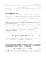
Therefore the special consideration is needed for electrodes. Fig. 6 shows two electrodes,
connected to an external harmonic voltage source with an amplitude V and a frequency

.


Fig. 6. Two electrodes, connected to an external harmonic voltage source with amplitude V
and frequency

.

First we will consider electrodes of zero thickness. Therefore all the mechanical values are
transferred without changes (electric potential is transferred without changes always by
metal layer of any thickness).
Values D
1
(1-) and D
1
(1+) on both sides of the first electrode are different, for the second
electrode analogously. The difference D
1
(1+) - D
1
(1-) is equal to the electric charge per unit
area of the electrode (in the SI system). A time derivative of this value is the current density.
Its multiplication on the electrode area A gives the total electrode current. For a harmonic
signal the time derivative equivalent to a multiplication on i

. As a result the following
expression takes place for a current I
1
of the electrode 1:
I
1
= i

A[D
1
(1+) - D
1
(1-)] (65)

For electrode 2 analogously. If there are only two electrodes connected to one electric source,
then I = I
1
= - I
2
and:
I = VY, (66)
where V =


–


(

1
and

2
are electrode potentials) and Y is an admittance of two
electrodes for the external electric source.
We are free in determining the zero point of the electric potential

and we can choose it so:

1
+

2
= 0, i.e. V = 2


1
= -2

2
(67)
Electrode 1

Electrode 2

x
1

D
1
(2+)

D
1
(
2-
)

D
1
(1-)

D
1
(1+)

V
I

Waves in Fluids and Solids

90
As a result, we can obtain from (65) and (66):

111
2
(1 ) (1 )
Y
DD
iA




(68)
which expresses the value of D
1
at the upper side of the electrode as a linear function of the
values of

and D
1
at the lower side (

has the same value on both sides of an electrode). It

means that the transfer matrix of the electrode of zero thickness (an ideal electrode) has a
following form:

Ee
100000 0 0
010000 0 0
001000 0 0
000100 0 0
000010 0 0
000001 0 0
000000 1 0
2
000000 1
Y
iA

















M
(69)
The metal electrode of a finite thickness (a real electrode) can be presented as a combination
of two layers, one of which is the metal electrode of a zero thickness (an ideal electrode),
transferring only electric values, and another one is a layer of a finite thickness, transferring
only the mechanical values (mechanical layer) - see Fig. 7.


Fig. 7. Representation of a real electrode as a combination of an ideal electrode and a
mechanical layer.
Therefore we can obtain the whole transfer matrix of the real electrode as a multiplication of
a matrix of the ideal electrode (69) and a matrix, transferring only mechanical values and
presented by expression (63):

M
E
= M
Ee
.
M
Em
= M
Em
.
M
Ee
(70)
As it was mentioned above, the matrices don’t obey the commutative law in general case,
but in this concrete case one can transpose these two matrices, what can be checked by

direct multiplication. This means, in particular, that an ideal electrode can be placed on any
side of the read electrode, as shown in Fig. 7. Physically more correctly to place the ideal
electrode on the side which is a face of contact with the interelectrode space.
As a result, the multilayer bulk acoustic wave resonator, containing arbitrary quantity of
arbitrary layers, but only with two electrodes, has a view, presented in Fig. 8.
=

=

real electrode

ideal electrode

mechanical la
y
er
mechanical la
y
er
ideal electrode

Surface and Bulk Acoustic Waves in Multilayer Structures

91


Fig. 8. Multilayer bulk acoustic wave resonator with two electrodes.
Here F is a combination of arbitrary quantity of arbitrary layers under electrodes, G is the
same above electrodes, Q is the same between electrodes (at least one of layers in Q must be
piezoelectric), E1 and E2 are the two electrodes of a finite thickness.

All the eight values u
j
, T
1j
, D
1
and

are transferring from a lower surface of the whole
construction to its upper surface by the whole transfer matrix, which is the multiplication of
transfer matrices of each elements:
M
FE1QE2G
= M
G
.
M
E2
.
M
Q
.
M
E1
.
M
F
(71)
Transfer matrices
M

F
, M
Q
, M
G
are calculated by (64) and matrices M
E1
and M
E2
– by (70).
Because of electrodes presence the total transfer matrix of the whole resonator
M
FE1QE2G
does
not have generally the special form with 0 and 1 in the 7
th
column and the 8
th
row (as in
(57)), but it is of the most general form:

11 12 13 11 12 13 1 1
21 22 23 21 22 23 2 2
31 32 33 31 32 33 3 3
11 12 13 11 12 13 1 1
12
21 22 23 21 22 23 2 2
uu uu uu uT uT uT u uD
uu uu uu uT uT uT u uD
uu uu uu uT uT uT u uD

Tu Tu Tu TT TT TT T TD
FE QE G
Tu Tu Tu TT TT TT T TD
MMMMMMMM
MMMMMMMM
MMMMMMMM
MMMMMMMM
MMMMMMMM
M





M
31 32 33 31 32 33 3 3
123123
123123
Tu Tu Tu TT TT TT T TD
uuuTTT D
Du Du Du DT DT DT D DD
MMMMMMM
MMMMMMMM
MMMMMMMM



















(72)
The expressions, obtained above, allow to calculate the admittance of the resonator Y which
is its main work characteristic.
The zero boundary conditions for T
1j
and D
1
on the external free lower and upper surfaces
of the construction are used for these calculations:
T
11
= 0, T
12
= 0, T
13
= 0, D
1
= 0 on free surfaces (73)

The normal components of a stress tensor are equal to zero because lower and upper
surfaces are free, the electric displacement is zero because the electric field of the external
source is concentrated only between two electrodes (between their inner surfaces).
E2


F

G
Q


x
1


E1


Waves in Fluids and Solids

92
Let us denote the mechanical displacements and the electric potential on the lower free
surface as
(1) (1) (1)
(1)
123
,,,uuu

and the same values on the upper free surface as

(2) (2) (2)
(2)
123
,,,uuu

. Then with taking into account (73) these values will be connected each
other by the transfer matrix
M
FE1QE2G
by the following expression:

(2)
11 12 13 11 12 13 1 1
1
(2)
21 22 23 21 22 23 2 2
2
(2)
31 32 33 31 32 33 3 3
3
11 12 13 11 12 13 1
(2)
0
0
0
0
uu uu uu uT uT uT u uD
uu uu uu uT uT uT u uD
uu uu uu uT uT uT u uD
Tu Tu Tu TT TT TT T

MMMMMMMM
u
MMMMMMMM
u
MMMMMMMM
u
MMMMMMM




















(1)
1
(1)

2
(1)
3
1
21 22 23 21 22 23 2 2
31 32 33 31 32 33 3 3
(1)
123123
123123
0
0
0
0
TD
Tu Tu Tu TT TT TT T TD
Tu Tu Tu TT TT TT T TD
uuuTTT D
Du Du Du DT DT DT D DD
u
u
u
M
MMMMMMMM
MMMMMMMM
MMMMMMMM
MMMMMMMM











































(74)
From here we can write for the 4
th
– 6
th
rows separately and for the 8
th
row separately:
(1)
1
11 12 13 1
(1)
(1)
21 22 23 2
2
(1)
31 32 33 3
3
0
0
0
Tu Tu Tu T
Tu Tu Tu T

Tu Tu Tu T
u
MMM M
MMM u M
MMM M
u























(1)

1
(1)
(1)
123
2
(1)
3
0( )
Du Du Du D
u
MMM u M
u









(75)
We can obtain the vector
(1) (1) (1)
123
,,uuufrom the first equation (75) (using the standard
inverse matrix designation):

1
(1)

1
11 12 13 1
(1)
(1)
21 22 23 2
2
(1)
31 32 33 3
3
Tu Tu Tu T
Tu Tu Tu T
Tu Tu Tu T
u
MMM M
uMMMM
MMM M
u











  







(76)
Now we can substitute this into the second equation (75) and obtain:

1
11 12 13 1
(1) (1)
123 212223 2
31 32 33 3
0( )
Tu Tu Tu T
Du Du Du Tu Tu Tu T D
Tu Tu Tu T
MMM M
MMM M M M M M
MMM M









     




(77)
In an arbitrary case

(1)
≠ 0, therefore we obtain from (77) the follow scalar equation:

1
11 12 13 1
123 21 22 23 2
31 32 33 3
() 0
Tu Tu Tu T
Du Du Du Tu Tu Tu T D
Tu Tu Tu T
MMM M
MMM M M M M M
MMM M













(78)
This is the main equation of the problem. It connects the resonator admittance Y with the
frequency

 because Y value is contained in the transfer matrices of electrodes. We can set

Surface and Bulk Acoustic Waves in Multilayer Structures

93
the concrete value of

and calculate from (78) the corresponding value of Y, i.e. we can
obtain the frequency response of the resonator – its main work characteristic. Matrix
elements in (78) are elements of the total transfer matrix of the whole device – see (72).
In an arbitrary case the equation (78) cannot be solved analytically. The solution can be
found only by some numerical method. We used our own algorithm of searching for the
global extremum of a function of several variables (Dvoesherstov et. al., 1999). Solution
corresponds to the global minimum of the square of the absolute value of the left part of the
equation (78). Two arguments of this function are the real and imaginary parts of the
admittance Y (for each given frequency).
If there is not any piezoelectric layer in the packets F and G outside the electrodes, the
transfer matrices of these packets have the simpler form (62) and the equation (78) can be
solved analytically in the following view:
1
()[ ]()
T u uu TT Tu uT uD TD D
QQ Q Q QQ
QQ Q

iA
Y

 


 
"" """"
FG FGFG
MMM MM MMM MMM MM M M
(79)
Here the compressed form of matrices is used for compactness. For example,
uu
Q
M means
the 3x3 matrix including the first 3 columns and the first 3 rows of the 8x8 matrix,
uT
Q
M
means the 3x3 matrix including the columns 4 – 6 and the first 3 rows of the 8x8 matrix,
T
Q

M means the 1x3 matrix including the columns 4 – 6 and the 7
th
row of the 8x8 matrix,
and so on. Index Q means that all these elements are taken from transfer matrix of the Q
packet (not for the whole device).
"
F

M
and
"
G
M
are 3x3 matrices, obtained as follows:

1
11
([(]
Em Em

  
"Tuuu
FF F
MM M M M))
1
22
[( ) ] ( )
TT Tu
Em Em

 
"
GG G
MMM MM (80)
In these expressions the lower indexes F and G also designate the corresponding packets,
M
F
and M

G
are the whole 8x8 matrices of the corresponding packets, M
E1m
and M
E2m
– the
“mechanical” parts of the electrodes 8x8 matrices and upper indexes uu, Tu, uT and TT
means that corresponding 3x3 matrices are taken from whole 8x8 matrices.
Practically all the concrete FBAR devices do not contain piezoelectric layers outside the
electrodes, i.e. practically for all these devices the frequency response can be calculated with
expressions (79) – (80).
But not only the frequency response can be calculated by the technique, described here. The
expression (57) allows to calculate all eight values u
j
, T
1j
, D
1
and

not only on the second
surface of the layer but also for any coordinate x
1
inside the layer, if these eight values are
known for the first “input” surface of this layer. These values on the second “output”
surface of the first layer can be used as “input” values for the second layer for the same
calculations for any coordinate x
1
inside the second layer and so on, i.e. the spatial
distribution of all eight values inside the whole multilayer system can be obtained. As was

mentioned above, the values on the first “input” surface of the first layer must be known for
such calculations (for frequency response calculations all eight values on the first surface of
the first layer are not needed).
Four of eight values, namely, T
1j
and D
1
are known, they are zero – see (73). The absolute
value of the electric potential is not essential from point of view of the spatial distribution of
all eight values. We can set any (but not zero) value of the electric potential on the first
surface of the first layer, for instance

(1)
= -1 V. Then we can obtain all three values of the
mechanical displacements
(1) (1) (1)
123
,,uuu from the equation (76). So all eight values on the

Waves in Fluids and Solids

94
first surface of the first layer are determined and the spatial distribution of all these values
can be obtained for any multilayer resonator with two electrodes. The admittance Y for
given frequency

must be calculated preliminary, because both these values are needed for
the spatial distribution calculation.
The spatial distribution gives a possibility to obtain some information about physical wave
processes those take place inside the multilayer structure, in particular - how the Bragg

reflector “works”.
Fig. 9 shows the frequency response of the membrane type resonator (as in Fig. 3a), obtained
by technique, described above. The mass density of all the materials are taken in a form (1 +
i)

, where  =-0.001 in this case. The frequency response is calculated for two variants of
the Al electrode thickness – zero and 0.1 m.


a) b)
Fig. 9. Frequency response of the membrane type resonator. Active layer – AlN, thickness 1
m. a) – zero electrode thikness, F
res
= 5.337 GHz, b) – Al electrode thickness 0.1 m, F
res
=
4.577 GHz. Electrode area 0.01 mm
2
.
Fig. 9 illustrates an influence of the electrode thickness on a resonance frequency (this
frequency is obtained directly from a graphic as coordinate of a maximum of a Y real part).
The resonance frequency is decreased by the electrodes of a finite thickness, because the
whole device with more total thickness corresponds to more half-wavelength. This
illustrates Fig. 10 in which the spatial distribution of the T
11
component of the stress tensor is
shown, obtained also by a technique, described above.


a) F = F

res
= 5.337 GHz b) F = F
res
= 4.577 GHz
Fig. 10. Spatial distribution of T
11
component of the stress tensor for two variants, shown in
Fig. 9. F = F
res
in both cases.

Surface and Bulk Acoustic Waves in Multilayer Structures

95
A half-wavelength corresponds to a distance between neighbouring points with zero stress.
In a case a) this distance is 1 m and corresponds to a resonance frequency 5.337 GHz,
whereas in a case b) a half-wavelength is equal to 1.2 m and corresponds to a lower
frequency 4.577 GHz. This gives a possibility to control the resonance frequency by
changing of the top electrode thickness. For example, Fig. 11 shows dependences of the
resonance frequency on a top electrode thickness for two materials of this electrode – Al and
Au. The bottom electrode is Al of a thickness 0.1 m in both cases.


Fig. 11. Dependences of the resonance frequency on the top electrode tickness for Al and Au.
The bottom electrode is Al (0.1 m) in both cases. The thickness of AlN is 1 m.
For displaying of the possibilities of the described method Fig. 12 shows also the spatial
distributions of the longitudinal component of the displacement u
1
and the electric potential


for the membrane type resonator, corresponding to Figs. 9b and 10b.


a) b)
Fig. 12. Spatial distribution of the longitudinal component of the displacement u
1
(a) and the
electric potential

(b) for the membrane type resonator with Al electrodes of finite thickness
0.1 m.
Distribution of D
1
is not shown here because it is very simple – D
1
= const between the
electrodes and equal to zero outside the inner surfaces of the electrodes.
If membrane type resonator is placed on the substrate of not very large thickness, then
multiple modes appear, and this resonator can be a multi-frequency resonator, as shown in
Fig. 13a.

Waves in Fluids and Solids

96

a) b)
Fig. 13. FBAR membrane type resonator on a Si substrate of thicness 100 m (a) and 1000 m
(b). Electrodes – Al, thicness 0.1 m, active layer – AlN, thickness 1 m.
But if the substrate is too thick, there are too many modes and the resonator transforms from
multi-mode actually into a “not any mode” resonator, as one can see in Fig. 13b.

So, the membrane type resonator cannot be placed on the massive substrate directly because
of an acoustic interaction with this substrate. One must to provide an acoustic isolation
between an active zone of the resonator and a substrate. One of techniques of such isolation
is a Bragg reflector between the active zone and the substrate (as shown in Fig. 3b). This
reflector contains several pairs of materials with different acoustic properties. The difference
of the acoustic properties of two materials in a pair must not be small. Acoustic properties of
materials, used for Bragg reflector, are characterized by a value

V, where

is a mass
density and V is a velocity. Values

V are shown in Fig. 14 for some isotropic materials.
Material constants are taken from (Ballandras et. al., 1997).


Fig. 14. The value

V for some isotropic materials.
As one can see in Fig. 14, the best combination for a Bragg reflector is SiO
2
/W. A pair Ti/W
is good too, and a combination Ti/Mo also can be used successfully (combinations of Au or
Pt with other materials also can be not bad, but not cheap).
The thickness of each layer of the reflector must be equal to a quarter-wavelength in a
material of the layer for a resonance frequency. As it was mentioned above, the resonance
frequency is defined mainly by the active layer thickness and can be adjusted by proper
choice of the top electrode thickness.

Surface and Bulk Acoustic Waves in Multilayer Structures

97
The computation technique, based on the described here rigorous solution of the wave
equations, allows to calculate any bulk wave resonators with any quantity of any layers,
including the resonators with Bragg reflector. For example, Fig. 15a shows a frequency
response of the resonator, containing an AlN active layer (1 m), two Al electrodes (both 0.2
m), three pairs of layers SiO
2
/W, and a Si substrate (1000 m).


a) b)
Fig. 15. A frequency response (a) and a distribution of u
1
(b) for a resonator with a Bragg
reflector, containing three pairs of layers SiO
2
/W.
A thickness of a Bragg reflector layer is 0.38 m for SiO
2
and 0.33 m for W (a quarter-
wavelength in a corresponding material for a resonance frequency). Fig. 15a shows, that
three pairs of SiO
2
/W combination is quite enough for full acoustic isolation of an active
zone and a substrate. A spatial distribution of a wave amplitude illustrates an influence of
the Bragg reflector on a wave propagation, for example, Fig. 15b shows this distribution for
a longitudinal component of a mechanical displacement. A coordinate axis x here is directed
from a top surface of a top electrode (x = 0) towards a substrate. One can see in Fig. 15b that

a wave rapidly attenuates in the Bragg reflector and does not reach the substrate.
Calculation results show, that the first layer after an electrode must be one with lower value

V – the SiO
2
layer in this case. In a contrary case a reflection will not take place.
If difference of values

V of two layers of each pair is not large enough, then three pairs may
not be sufficient for effective reflection. For example, calculations show that three or even
four pairs of Ti/Mo layers are not sufficient for suppressing the wave in the substrate. Only
five pairs give a desired effect in this case and provide results similar shown in Fig. 15 for
SiO
2
/W layers.
So, the described technique allows to calculate any multilayer FBAR resonators, containing
any combinations of any quantity of any layers. The main results of these calculations are a
frequency response of a resonator and spatial distributions of physical characteristics of the
wave (displacement, stress, electric displacement and potential).
In addition this technique gives a possibility to calculate a thermal sensitivity of the
resonator too, i.e. an influence a temperature on a resonance frequency. A resonance
frequency always changes in general case when a temperature changes. This change is
characterized by a temperature coefficient of a frequency:

1
r
r
dF
TCF
FdT

 (81)

Waves in Fluids and Solids

98
Here T is a temperature, F
r
is a resonance frequency.
A computation technique, used here, allows to apply this expression for TCF calculation
directly and to calculate this value by numerical differentiation.
A temperature influence on a resonance frequency is due to three basic causes:
1.
A temperature dependence of material constants (stiffness, piezoelectric, dielectric
tensors) - TCF
C

2.
A temperature dependence of a mass density – TCF


3.
A temperature dependence of a layer thickness – TCF
h

A temperature dependence of material constants is described by temperature coefficients of
these constants, a temperature dependence of a mass density is described by three linear
expansion coefficients or by a single bulk expansion coefficient, a temperature dependence
of a thickness is described by a linear expansion coefficient along a thickness direction. All
these coefficients can be found in a literature, for example, for materials, usually used for
FBAR resonators, one can see corresponding values in (Ivira et al., 2008).

First we will consider the simplest variant – a membrane type FBAR resonator with a single
AlN layer and infinite thin electrodes. For typical values of AlN temperature coefficients we
can easily obtain:
TCF = TCF
c
+ TCF

+ TCF
h
= (-29.639 +7.343 – 5.268)
.
10
-6
/
о
С = -27.564
.
10
-6
/
о
С
One can check by a direct calculation, that this result does not depend on a thickness of AlN
layer (for this variant with electrodes of finite thickness and for any multilayer structure
with layers of finite thickness it is not so). TCF

value is always positive, TCF
h
value is
always negative. A sign of TCF

c
is defined mainly by a sign of temperature coefficients of
stiffness constants. If temperature coefficients of stiffness constants are negative (for most
materials, including AlN), then TCF
c
is negative, if temperature coefficients of some stiffness
constants are positive (rare case, for example quartz), then TCF
c
can be positive and a total
TCF can be zero.
For AlN a TCF value is always negative. Al electrodes aggravate this position, besause
temperature coefficients of Al stiffness constants are negative too. From this point of view
Mo electrodes are more preferable, because absolute values of temperature coefficients of
its stiffness constants are significantly less than ones for Al (althouth they are also
negative). For example, the concrete membrane type resonator Al/AlN/Al with an Al
thickness 0.2 m and an AlN thickness 1.1 m we can obtain: TCF = -44.23
.
10
-6
/
о
С (F
r
=
3.648 GHz), and for Mo/AlN/Mo resonator with the same geometry: TCF = -33.76
.
10
-6
/
о

С
(F
r
= 2.615 GHz).
For most applications a resonator must be thermostable, i.e. TCF must be equal to zero. The
single possibility to compensate the negative TCF of AlN and of electrodes and to provide a
total zero TCF is to add some additional layer with positive temperature coefficients of
stiffness constants. Such material is, for example SiO
2
. Fig. 16 shows dependenses of TCF of
membrane type resonator with Mo electrodes on a thickness h
t
of a SiO
2
layer for two cases:
SiO
2
layer is placed together with AlN layer between electrodes (structure
Mo/SiO
2
/AlN/Mo) and SiO
2
layer is placed outside the electrodes (structure
SiO
2
/Mo/AlN/Mo). Corresponding dependences of a resonance frequency are presented in
Fig. 16 too.
Fig. 16 shows that a SiO
2
layer more effectively influences on both TCF and a resonance

frequency, when it is placed between electrodes.

Surface and Bulk Acoustic Waves in Multilayer Structures

99

a) b)
Fig. 16. Dependences of TCF and a resonance frequency on a SiO
2
layer thickness h
t
for
cases, when SiO
2
is placed between electrodes (a) and when SiO
2
is placed outside electrodes
(b). A thickness of Mo electrodes is 0.06 m, a thickness of AlN is 1.9 m.
Calculations show that a Bragg reflector does not change a resonance frequency of the
corresponding membrane type resonator, if a thickness of each layer of the reflector is exactly
equal to a quarter-wavelength. But a Bragg reflector influences on a TCF. For this reason it is
reasonable to choose SiO
2
as one material of a reflector. In this case a thickness of an additional
compensating SiO
2
layer can be reduced. For example, a thickness of SiO
2
layer outside
electrodes, corresponding to TCF = 0, is equal about 0.53 m for variant, shown in Fig. 16b for

membrane type resonator. A resonance frequency is about 2.11 GHz for this case. The Bragg
reflector with three pairs of SiO
2
/Mo, corresponding this frequency, does not change this
frequency, but a TCF becomes positive due to SiO
2
material presense in the reflector. One must
reduce a thickness of an additional compensating SiO
2
layer to return a TCF to zero. But then a
resonance frequency will increase. We must either increase an AlN layer thickness to return a
resonance frequency or to change thickness of a Bragg reflector layers to adjust the reflector to
a new resonance frequency. In any case several steps of sequential approximation are
necessary. The technique, described here, allows to do this without problem. For example,
presented in Fig. 16b, full thermocompensation can be obtained for h
t
= 0.4 m (instead of 0.53
m for membrane type resonator) and for thickness of SiO
2
and Mo layers in a Bragg reflector
0.71 m and 0.75 m respectively. The AlN layer thickness remains 1.9 m and a resonance
frequency slightly shifts remaining in the vicinity of 2.1 GHz.
In many cases a presentation of FBAR resonator by means of some equivalent circuit is
convenient – see for example (Hara et. al., 2009). The simplest variant of an equivalent
circuit is shown in Fig. 17.


Fig. 17. An equivalent circuit of FBAR resonator.
C
m

L
m
R
m

C
0


Waves in Fluids and Solids

100
Hear C
0
is a static capacitance of a resonator – a real physical value, which can be calculated
by the geometry of the resonator and the dielectric properties of the layers between the
electrodes:

1
0
0
1
1
m
i
i
i
l
C

A









(82)
where

i
and l
i
is a relative dielectric permittivity (element

11
of a tensor) of a layer number i
and its thickness,

0
= 8.854
.
10
-12
F/m – the dielectric constant, A is an area of a resonator
electrode, m is a quantity of layers between electrodes.
Values C

m
, L
m
, and R
m
are equivalent dinamic capacitance, inductance and resistance of the
resonator – values, which can not be determined from any physical representation – only by
comparison with experimental frequency response or with response, obtained by some exact
theory. Theory, described here, allows to obtain these values.
An admittance of the equivalent circuit, shown in Fig. 17, can be calculated by following
expressions:

1
0Im0
1
em m Rm
m
YjL R jCYYjC
jC








(83)
Here

2
2
1
m
Rm
mm
m
R
Y
LR
C








Im
2
2
1
1
m
m
mm
m
L
C

Yj
LR
C










(84)
Y
Rm
and Y
Im
are an active and reactive components of a dinamic admittance of the resonator,
j

C
0
is an admittance of the static capacitance.
Comparison of admittance, calculated by (83) and (84), with admittance, calculated by a
rigorous theory, described here, allows to obtain the unique values C
m
, L
m
, and R

m
, which
give a frequency response, equivalent to the response, given by the rigorous theory.
The resonance frequency of the equivalent circuit, shown in Fig. 17, is defined as:

1
2
rr
mm
F
LC

 (85)
The value R
m
corresponds to a maximum of the active component of the admittance (see (84)):

max
1
()
m
Rm
R
Y
 (86)
We can find a quality-factor from curve of a active component of the admittance:

r
F
Q

F


(87)

Surface and Bulk Acoustic Waves in Multilayer Structures

101
Here F is a full width of the curve at a level 0.5 of a maximum.
Then we can calculate an equivalent dynamic inductance:

2
m
m
r
QR
L
F

 (88)
At last we can calculate an equivalent dynamic capacitance with help of (85):

2
1
(2 )
m
mr
C
LF



(89)
All these calculations the computer program performs automatically and shows obtained
results in corresponding windows of the program interface (a program is made in a Borland
C++ Builder medium and provides automatic transfer of main results into Excel worksheet).
A frequency response, calculated by expressions (83) and (84) with values C
m
, L
m
, R
m
,
obtained by such a manner, practically coincides with a frequency response, calculated with
rigorous theory, described here (if there is only one resonance peak in a frequency range). In
a wide frequency range may be several resonance peaks. In this case one can connect
required quantity of C
m
, L
m
, R
m
circuits in parallel (but with only one C
o
for all them) in Fig.
17. C
m
, L
m
, R
m

values for every circuit can be determined by comparison with corresponding
peak, given by a rigorous theory.
4. Conclusion
General methods of surface and bulk acoustic wave in multilayer structures calculation are
described in this chapter. Corresponding equations are formulated. These equations allow
to calculate all the main wave propagation characteristics and the device parameters. A
phase velocity, an electromechanical coupling coefficient, a temperature coefficient of delay,
a power flow angle and others for surface wave devices and a frequency response, a spatial
distribution of the wave characteristics, a resonance frequency, a temperature coefficient of
frequency, parameters of an equivalent circuit for bulk acoustic resonators are available for
calculations by described techniques. Obtained results allow better to understand processes
taking place in these devices and to improve their characteristics. Corresponding algorithms
and computer programs can be used for design of surface and bulk acoustic wave devices.
5. References
Adler, E.L. (1994). SAW and pseudo-SAW properties using matrix methods, IEEE
Transactions on Electronics, Ferroelectrics, and Frequency Control., Vol. 41, No. 6,
(November 1994), pp. (876-882).
Ballandras, S.; Gavignet, E., Bigler, E., and Henry, E. (1997). Temperature Derivatives of the
Fundamental Elastic Constants of Isotropic Materials, Appl. Phys. Lett. Vol. 71, No.
12, (September 1997), pp. (1625-1627).
Campbell, J. J. & Jones, W.R. (1968). A method for estimating optimal crystal cuts and
propagation directions for excitation of piezoelectric surface waves, IEEE
Transactions on Sonics and Ultrasonics, Vol. 15, No. 4, (October 1968), pp. (209-217).

Waves in Fluids and Solids

102
Dvoesherstov, M.Y., Cherednick, V.I., Chirimanov, A.P., Petrov, S.G. (1999). A method of
search for SAW and leaky waves based on numerical global multi-variable
procedures, SPIE Vol. 3900, pp. (290-296).

Hara, M.; Yokoyama, T., Sakashita, T., Ueda, M., and Satoh, Y. (2009). A Study of the Thin
Film Bulk Acoustic Resonator Filters in Several Ten GHz band, IEEE International
Ultrasonics Symposium Proceedings, (2009), pp. (851-854).
Ivira, B.; Benech, P., Fillit, R., Ndagijimana, F., Ancey, P., Parat, G. (2008). Modeling for
Temperature Compensation and Temperature Characterizations of BAW
Resonators at GHz Frequencies, IEEE Transactions on Ultrasonics, Ferroelectrics, and
Frequency Control, Vol. 55, No. 2, (February 2008), pp.(421-430).
Kovacs, G., Anhorn, M., Engan, H.E., Visiniti, G. and Ruppel, C.C.W. (1990). Improved
Material Constants for LiNbO
3
and LiTaO
3
, IEEE International Ultrasonics
Symposium Proceedings, (1990), pp. (435-438).
Nowotny, H. & Benes, E. (1987). General one-dimensional treatment of the layered
piezoelectric resonator with two electrodes, Journal of Acoustic. Society of America,
Vol. 82 (2), (August 1987), pp. (513-521).
Shimizu, Y.; Terazaki, A., Sakaue, T. (1976). Temperature dependence of SAW velocity for
metal film on -quartz, IEEE International Ultrasonics Symposium Proceedings, (1976),
pp. (519-522).
Shimizu, Y. & Yamamoto, Y. (1980). Saw propagation characteristics of complete cut of
quartz and new cuts with zero temperature coefficient of delay, IEEE International
Ultrasonics symposium Proceedings, (1980), pp. (420-423).
4
The Features of Low Frequency Atomic
Vibrations and Propagation of Acoustic
Waves in Heterogeneous Systems
Alexander Feher
1
, Eugen Syrkin

2
, Sergey Feodosyev
2
, Igor Gospodarev
2
,
Elena Manzhelii
2
, Alexander Kotlar
2
and Kirill Kravchenko
2

1
Institute of Physics, Faculty of Science P. J. Šafárik University, Košice
2
B.I.Verkin Institute for Low Temperature Physics and Engineering NASU, Kharkov
1
Slovakia
2
Ukraine
1. Introduction
In recent years, the quasi-particle spectra of various condensed systems, crystalline as well
as disordered and amorphous, became also the “object” of applications and technical
developments and not only of fundamental research. This led to the interest in the
theoretical and experimental study of the quasi-particle spectrum of such compounds,
which are among the most popular and advanced structural materials. Most of these
substances have heterogeneous structure, which is understood as a strong spatial
heterogeneity of the location of different atoms and, consequently, the heterogeneity of local
physical properties of the system, and not as the coexistence of different phases (i.e.

heterophase). To these structures belong disordered solid solutions, crystals with a large
number of atoms per unit cell as well as nanoclusters.
This chapter is devoted to the study of vibration states in heterogeneous structures. In such
systems, the crystalline regularity in the arrangement of atoms is either absent or its effect
on the physical properties of the systems is weak, affecting substantially the local spectral
functions of different atoms forming this structure. This effect is manifested in the behavior
of non-additive thermodynamic properties of different atoms (e.g. mean-square amplitudes
of atomic displacements) and in the contribution of individual atoms to the additive
thermodynamic and kinetic quantities. The most important elementary excitations
appearing in crystalline and disordered systems are acoustic phonons. Moreover, in
heterogeneous nanostructures the application of the continuum approximation is
significantly restricted; therefore we must take into account the discreteness of the lattice.
This chapter contains a theoretical analysis at the microscopic level of the behavior of the
spectral characteristics of acoustic phonons as well as their manifestations in the low-
temperature thermodynamic properties.
The chapter consists of three sections. The first section contains a detailed analysis at the
microscopic level of the propagation of acoustic phonons in crystalline solids and
disordered solid solutions. We analyze the changes of phonon spectrum of the broken
crystal regularity of the arrangement of atoms in the formation of a disordered solid

Waves in Fluids and Solids

104
solution with heavy isotope impurities and randomly distributed impurities weakly
coupled both with the atoms of the host lattice and among themselves. As is well known,
such defects enrich the low-frequency phonon spectrum and lead to a significant change in
the low-temperature thermodynamic and kinetic characteristics (see, for example, Kosevich,
1999; Maradudin et al., 1982; Lifshitz, 1952a). In particular, the impurity atoms cause the so-
called quasi-localized vibrations (Kagan & Iosilevskij, 1962; Peresada & Tolstoluzhskij 1970,
1977; Cape et al., 1966; Manzhelii et al., 1970). This section analyzes in detail the conditions

of the formation and evolution of quasi-localized vibrations with increasing concentration of
impurities. It is shown that the quasi-local maximum in the phonon spectrum of the low-
frequency zone is formed by vibrations localized on impurity atoms. Rapidly propagating
phonons corresponding to the vibrations of the host lattice atoms are scattered by localized
vibrations. This scattering forms a kink in the local spectral densities of these atoms that is
similar in shape to the first van Hove singularity of a perfect crystal. In the description of the
spectral characteristics of the elementary excitations in heterogeneous structures such
theoretical methods are necessary which do not involve the translational symmetry of the
crystal lattice. In this section we use such a method for computing the local Green's
functions and the local and partial spectral densities.
These self-averaging spectral characteristics (Lifshitz et al., 1988) can be determined also for
compounds that do not possess regularity in their crystal structure. An effective method for
describing disordered systems and calculating their quasi-particle spectra is the method of
Jacobi matrices (
J -matrices) (Peresada, 1968; Peresada et al., 1975, Haydock et al., 1972). By
this method the majority of the calculations in this paper were carried out
.
The second section is devoted to the analysis of the reasons for the strong temperature
dependence of the Debye temperature Θ
D
(T) under T ≤ 0.1Θ
D
. The temperature dependence
Θ
D
(T) is a solution of the transcendental equation C
D
(T/Θ
D
) = C(T), where C(T) is calculated

at the microscopic level or experimentally determined and C
D
(T/Θ
D
) is the temperature
dependence of the Debye heat capacity. It is shown that the reason for the formation of a
low-temperature minimum on the dependence Θ
D
(T) are the fast-propagating low-
frequency phonons (propagons) (Allen et al., 1999) scattered on the slow quasi-particles. In
the case of a defect (random reduction of force constants) the quasi-localized vibrations do
not form, but in the ratio of the phonon density of states ν(ω) to the square of the frequency
a maximum in the propagon zone of the phonon spectrum is formed with increasing
concentration of defects. The maxima in the ratio ν(ω)/ω
2
are called boson peaks (see, for
example, Feher et al., 1994; Gurevich et al., 2003; Schrimacher et al., 1998). They are
intensively studied for systems with topological disorder, glasses and such compounds as
molecular crystals with rotational degrees of freedom. In this section we analyze the arising
of such features in solid solutions with only vibration degrees of freedom. The frequency of
the boson peak coincides with the frequency of the quasi-local vibrations corresponding to a
weakly bound impurity at concentrations, for which the average distance between the
randomly distributed impurity atoms corresponds to the propagon frequency equal to the
frequency of quasi-local vibrations. That is, the distance between the impurities (disorder
parameter) becomes comparable to the wavelength of rapid acoustic phonons with the
frequency equal to the quasi-local vibration frequency. This corresponds to the phonon
Ioffe-Regel crossover (Klinger & Kosevich, 2001, 2002). It is shown that the temperature-
dependence and magnitude of Θ
D
(T) are even more informative than the phonon density of

states. It was shown on the example of a Kr
1-p
Ar
p
solid solution that for p ≈ 25% there are no
singularities both in the propagon zone of the phonon density of states and in the phonon
The Features of Low Frequency Atomic Vibrations
and Propagation of Acoustic Waves in Heterogeneous Systems

105
density relation to the square of frequency. At the same time, the temperature dependence
of the relative (compared with pure Kr) changes in the low-temperature heat capacity shows
two peaks that can not be explained by the superposition of contributions of isolated
impurities, impurity pairs, etc. The reason of this behavior is the scattering of fast
propagating phonons, corresponding to the krypton atoms, on significantly slower phonons
corresponding to the vibrations of atoms in argon clusters.
Many features of the phonon spectra and vibrational characteristic of disordered
heterogeneous structures are also inherent to the crystals with polyatomic unit cells. Third
section of this work is devoted to the analysis of phonon spectra and vibrational
characteristics of such crystals. The manifestations of the phonon Ioffe-Regel crossover in
multilayered regular crystalline structures are analyzed. The presence of the quasi-two-
dimensional and quasi-one-dimensional features in the behavior of the vibrational
characteristics of multilayer compounds is shown. The macroscopic characteristics of such
compounds are derived from the low-dimensional ones. This allows us to describe the
vibrational characteristics of such complex compounds in frames of low-dimensional
models. The features of the interaction of phonons with a planar defect are investigated
using these models. In particular, the resonance effects in the scattering of acoustic waves
and the formation of localized and resonance vibrational states in the planar defect are
considered. Such effects may lead to singularities in the experimentally observed kinetic
characteristics of the grain boundaries. The heat transfer between two different media, on

the condition that the Fano resonance occurs, is analyzed.
2. Low-frequency characteristics of the phonon spectra of disordered solid
solutions
This chapter is devoted to the study of the propagation of acoustic phonons at different
frequencies of quasi-continuous FCC crystal phonon spectrum. We analyze in more detail
the analogy of the Van Hove singularity in the phonon spectrum of the perfect crystal with
similar features of the phonon spectra of structures with broken regularity in the
arrangement of atoms of a crystal. For any solid (both crystal and the one which does not
possess the translational symmetry of the atoms arrangement), a low-frequency range exists
where the dispersion relation of phonons has the form




sk

k

( k is a module of the
wave vector k ,
k

k

, and


s

is the velocity of sound). The phonon density of states in

this range takes the Debye form

2
~

. With the increase of the k -value the phonon
dispersion relation increasingly deviates from the linear one (frequency

becomes lower
than
sk ) and the actual density of states deviates upwards from the Debye one. At low
frequencies, the sound propagation occurs along all crystallographic directions. With
increasing frequency the propagation velocity of acoustic phonons decreases, this decrease
being different for different crystallographic directions. In a perfect crystal, when the
phonon frequency corresponds to the frequency of the first van Hove singularity *
 ,
the propagation of the transverse sound along one of the crystallographic directions (in the
FCC it is the crystal direction
ГL, Fig. 1a) ceases and the corresponding group velocity is
zero. Phonons with frequencies *

 were named propagons and those with higher
frequencies are called
diffusons. With a further frequency increase also the number of
directions increases along which the propagation of sound ceases. The highest frequency of
the van Hove singularity ( * *

 ) corresponds to the frequency at which the wavelength

Waves in Fluids and Solids

106
of the longest wavelength phonons is smaller than the interatomic distance (Fig. 1b).
Phonons with * * are almost localized and they were named locons, while the
frequency interval


**,
m

 is called the locon band.


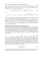
Fig. 1.
The phonon density of states (red lines), the frequency dependences of the group
velocities of phonon modes (part
a) and frequency dependences of the values


0
/
eff
l
(part
b) along the main of the highly symmetrical crystallographic directions of FCC crystal
with central nearest-neighbors interaction (blue, purple and olive line, depending on the
direction). The first octant of the first Brillouin zone of a FCC crystal with indications of
considered high-symmetry directions is shown on the right (
0
2la is the distance

between nearest neighbors).
Note that the propagation character of locons and diffusons practically does not differ from
the propagation character of optical phonons in a crystal with complex lattice. A
translational symmetry disturbance does not lead to a qualitative modification in the nature
of acoustic phonons and does not change their classification.
Let in the crystal randomly introduce heavy isotopic substitution impurities or impurities
weakly coupled to the atoms of the host lattice and among themselves. Neglecting the
interaction between impurities the variations of the phonon spectrum are satisfactorily
described by the theory of regular perturbations devised by I.M. Lifshitz (Lifshitz, 1952a). In
particular, the formation of the so-called quasi-local vibrations (QLV) due to the presence of
heavy or weakly bound impurities was predicted (Kagan & Iosilevskij, 1962) and studied in
detail both theoretically (see, for example, Peresada & Tolstoluzhskij 1977) and
experimentally (see, for example, Cape et al., 1966; Manzhelii et al., 1970). The QLV are
manifested by the resonance peaks in the low-frequency part of the phonon spectrum and
they contribute essentially to the low-temperature thermodynamic properties. At low
impurity atoms concentrations
1p

 , the vibration characteristics of the solid solution can
be described within the linear in p approximation:

 


i
i
p

  



(1)
The summation is performed over all cyclic subspaces (Peresada, 1968; Peresada et al.,1975),
in which the operator
ˆ

describing the perturbation of the lattice vibrations by either
isolated heavy or weakly coupled impurity is non-zero,


i

 is the spectral density
The Features of Low Frequency Atomic Vibrations
and Propagation of Acoustic Waves in Heterogeneous Systems

107
change in each of these subspaces,





and



 are the phonon densities of solid
solution and perfect crystal states, respectively. If in each of the cyclic subspaces the
operator

ˆ
 induces a regular degenerate operator, then the value



i

 can be
calculated using the spectral shift function



 (Lifshitz, 1952a). Using the expressions
obtained for this function in the J-matrix method (Peresada, 1968; Peresada et al., 1975,
Peresada & Tolstoluzhskij 1977), we obtain:




  
 

2
2
22
Re
Re
dSG
d
dd

SG



 
     





   



(2)

where the function


S

describes the perturbation by defect and depends on the defect
parameters,


G  is the local Green’s function of a perfect crystal. If in any cyclic subspace
the solution of the equation






Re 0SG

 (3)
is
k
 , then in the vicinity of this value the expression (2) has a resonant character:




 
2
2
2
;
4
Re
k
k
d
d
d
SG
d


 


 

 
 


. (4)
The equation (3) formally coincides with the Lifshitz equation which yields (of course for
other values of


S

) the frequencies of discrete vibrational levels, lying outside the band of
quasi-continuous spectrum of the crystal (Lifshitz, 1952a). However, these discrete levels
are, in contrast to the values
k

, the poles of the perturbed local Green’s function. The
Green’s function can not have poles within the quasi-continuous spectrum. The possibility
to determine the QLV frequencies using equation (3) arises from the fact that at low
frequencies




00 00
Re ImGG


  .
Let us analyze the quasi-local oscillations due to the substitution impurity in an FCC crystal
with the central interaction of nearest-neighbors. The interaction of the impurity with the host
lattice is also considered as a purely central and, therefore, the perturbation caused by such an
impurity should be regular and degenerate. Let us consider two cases: the isotopic impurity
with a mass four times higher than that of the host lattice (i.e. the mass defect is 3mm  )
and the impurity atom with a mass equal to the mass of a host lattice atom  = 0 and coupled
to the host lattice four times weaker than are the atoms of the host lattice between each other
( 34  is the coupling defect). In the first case, operator
ˆ

induces a non-zero
operator only in the cyclic subspace which is generated by the displacement of the impurity
atom. The vectors corresponding to this subspace transform according to the irreducible
representation
5

 of the symmetry group of the lattice
h
O (the notation of Kovalev, 1961). In
the given subspace the spectral density of perfect lattice coincides with its density of states. For
an isotopic impurity the function


S

(Peresada & Tolstoluzhskij, 1977) reads:


2

is
S 


(5)

Waves in Fluids and Solids

108
In the second case, except the subspace
5
()
H


where the function


S

is





5
2
3
1

2
m
w
S




 


(6)
the non-zero operators will be operators induced by the operator
ˆ

in cyclic subspaces
transformed according to irreducible representations,
1


,
3


,
4


and
4



of the same group
h
O . Over all of these four subspaces



2
16
m
S

. For weakly bound impurity, the
function
lim
16 /
wm
SS


 and equation (3) can not have solutions in the propagon zone
within these cyclic subspaces. Therefore, for real values of parameter

equation (3) has a
solution in the subspace
5
()
H



only. This solution for both cases shows Fig. 2. The real part of
the Green’s function (curves 2 in both parts) crosses the dashed curves 3, which represent the
equations (5) (part
a) and (6) (part b), at points
k

. This figure also shows the spectral
densities

5
()


 of the perfect crystal, coinciding with its phonon density of states




(dashed curves 1), and phonon densities of states of the corresponding solid solutions with
concentration
5%p  . This figure shows the phonon density of states (curves 1) for both the
heavy isotopes (part a) and weakly bound impurities (part b). Curves 4 show the
contributions from impurities and curves 6 those from the matrix lattice. We can see that the
maxima formed on the phonon densities


,
p



are (curves 1) completely caused by the
vibrations of impurity atoms. Let us analyze figures 2 and 3 together. The value of the
phonon density of states of a perfect crystal at
k

 can not be considered as negligible,
since it is comparable to the value of the real part of the Green’s function at this frequency
(




~0.1Re
kk
G 
). Therefore, as is seen from the figures, though the frequencies of the
maxima on the curves


,
p


and


,
imp
p


are close to the frequency
k

, they do not
coincide with it (Fig. 2
b) (especially in the case of a weakly bound impurity). For weakly
bound impurity one should expect a higher degree of localization of QLV on impurity
atoms. In Fig. 3 the values of


,
imp
p

are compared with the spectral density of isolated
impurity atoms



5
55
1
() ()
2
00
2
ˆ
ˆ
Im ,hILh









 








. The function


,
imp
p

is
nonzero only near frequencies
ql

, which are the maxima on curves 5. Therefore the
frequency

ql
 can be more reasonably than
k

considered as the frequency of QLV (quasi-
local frequency).
Therefore, QLV can be represented as waves slowly diverging from the impurity, similar to
spherical waves. Fig. 2 also presents (curves 4) the values of

5
()
01



 , i.e. the spectral
correlators of displacements of impurity atoms with their first coordination sphere




55 55
1
() () () ()
22
1
01 1 0
2
ˆ
ˆ

Im ,hILhP
 

 



  







, (8)
The Features of Low Frequency Atomic Vibrations
and Propagation of Acoustic Waves in Heterogeneous Systems

109

Fig. 2. Phonon densities of disordered solid solutions with impurity concentration 5% (curves
1) and solutions of the equation (3) (intersection of curves 2 and 3) for cases of a heavy isotopic
impurity (part
a) and weakly bound impurities (part b). Curves 4 in both parts are spectral
correlators of vibrations of the impurity atom with its first coordination sphere.
where


2

1
P  is the polynomial defined by the recurrence relations for the J-matrix of the
perturbed operator
ˆ
ˆ
L+

(Peresada, 1968; Peresada et al.,1975). Spectral correlator


01

vanishes when

E
= , where
E

is the Einstein frequency of the correspondent subspace
(

22
0
m
E
d

  

). Thus, when



E
= , the correlation with the first coordination sphere is
absent, and the close is the frequency

ql
to

E
, the stronger is the degree of localization of
QLV. As it could be seen from Fig. 2 the QLV frequency for weakly bound impurity is
nearly three times closer to

E
than that the heavy isotopic one, and the quasi-local
maximum for a weakly bound impurity has a sharper resonance form than the maximum
for a heavy isotopic defect.
The QLV are localized near the impurity atoms and their formation is very similar to the
occurrence of discrete vibrational levels (local oscillations) outside the continuous spectral
band of the host lattice in the presence of light or strongly coupled impurities in a crystal.
However, there is an important fundamental difference between the local and quasi-local
vibrations, manifested under increasing concentration of impurity atoms. Local vibrations
are the poles of the Green’s function of the perturbed crystal, and their amplitudes decay
exponentially with the distance from the impurity. Being located outside the quasi-
continuous spectrum, these vibrations do not interact with the phonon modes of the host
lattice. With an increasing concentration of either light or strongly coupled impurities their
effect upon phonon spectrum can be determined by taking into account the expansion of
concentration (Lifshitz et al., 1988). Thus, the increase of the concentration of light impurities
leads to the appearance of sharp resonant peaks in phonon spectrum with frequencies

coincident with those of local vibrations of the isolated impurity atom pairs and eventually,
regular triangles and tetrahedrons (Kosevich et al., 2007). The QLV are not the poles of the
Green’s function, they are common non-divergence maxima in the phonon density of states.
Though, as is shown in the next section, these peaks are formed by the impurity atoms
vibrations which interact with the phonon modes of host lattice. Therefore, at finite (even
low enough, about few percents) concentrations of heavy or weakly coupled impurity atoms,
the significant modification of the entire phonon spectrum of the crystal occurs,

Waves in Fluids and Solids

110


Fig. 3. Phonon densities of disordered solid solutions with impurity concentration 5%
(curves 1); from contributions impurity atoms (curves 4) and atoms of the host lattice
(curves 6). Part
а corresponds to the heavy isotopic impurity ( 4mm


), part b corresponds
to a weakly bound impurity ( 14


 ). Curves 2 show the phonon density of the original
perfect lattice, curves 3 represent the frequency dependence of the transverse sound velocity
along the crystallographic direction ГL, and curves 5 show the spectral density of single
isolated impurities, multiplied by the concentration
0.05p

.

which can not be described by the expansion of the impurity concentration. Thus the
weakening of bonds between the argon impurities in krypton matrix leads to a characteristic
“two-extreme” behavior of the temperature dependence of the relative change in the low-
temperature heat capacity unexplained by the superposition of contributions of isolated
impurities, impurity pairs, triples and etc., without taking into account the restructuring of
the entire spectrum (Bagatskii et al., 2007). The restructuring of the phonon spectrum of the
crystal and the delocalization of QLV at finite concentrations of impurities in the coherent
potential approximation was considered in (Ivanov, 1970; Ivanov & Skripnik, 1994).
The QLV usually occur in the frequency range where corresponding wavelengths of
acoustic phonons of the host lattice become comparable to the average distance between the
defects (the so-called disorder parameter). This is valid even for low concentrations of
impurity atoms as is illustrated in Fig. 1b. The value


ql


for most phonon modes
exceeds the disorder parameter even at 1%p

. Therefore an interaction of QLV with
rapidly propagating acoustic phonons of the host lattice (propagons) appears as the Ioffe-
Regel crossover as is shown in (Klinger & Kosevich, 2001, 2002) and can lead to the
formation of a boson peak (BP). The BP is an anomalous override of the low-frequency
phonon density over the Debye density. The BP was observed in the Raman and Brillouin
scattering spectra (Hehlen et al., 2000; Rufflé et al., 2006) and in inelastic neutron scattering
experiments (Buchenau et al., 1984) as maxima in the frequency dependence

2
  or


2
I  (


I  is the scattering intensity). These peaks appear in the low-frequency region
(between 0.5 and 2 THz) of the vibration density of states (Ahmad et al., 1986), i.e. far below
the Debye frequency. At the BP frequency the transition occurs from the fast-propagating
low-frequency phonons (propagons), with dispersion relation close to the acoustic one, to
The Features of Low Frequency Atomic Vibrations
and Propagation of Acoustic Waves in Heterogeneous Systems

111
the so-called diffusons, i.e. phonons, whose propagation is hampered by the scattering on
localized states (Feher et al., 1994). In the frequency range


***
,

 , the number of localized
vibrations increases with the frequency increase (Fig. 1a). Therefore, the phonons with
frequencies lying in that interval (diffuson area) are either diffusons or locons. The similarity
of the boson peak in disordered systems (e.g. glasses and substitution solid solutions) to the
first van Hove singularity in crystal structures is noted in (Buchenau et al., 2004;
Gospodarev et al., 2008). BPs are also observed in polymeric and metallic glasses (Duval et
al., 2003; Arai et al., 1999).
As is shown in Fig.4 in the frequency range [
*
0, ] the vibrations of atoms of the host lattice

propagate rapidly and are scattered by the quasi-localized states formed by impurity
vibrations. Curves 6 in this figure depict the frequency dependence


,,
imp
p
p  

. At
frequencies
ql
 there vibrations propagate as plane waves. Corresponding parts of
curves 6 are smooth and have parabolic (quasi-Debye) form. At
ql

 a kink similar to the
shape of the first van Hove singularity can be seen on curves 6. At this frequency as well as
at *
 in the phonon spectrum of a perfect crystal (Fig. 1a) there is a sharp change of the
average group velocity of phonons. The frequency
ql

is the upper limit of propagon zone
of solid solution. This is clearly exhibiting with increasing impurity concentration p. Fig. 4
shows the evolution of the contribution to the phonon density of states by the displacements
of impurity atoms (part
a) and by the displacements of atoms of the host lattice (part b) with
increasing impurity concentration. Note that both dependences can be determined
experimentally (e.g., by the method described in (Fedotov et al., 1993). On both parts of

Fig. 4 dashed curves show phonon densities of states of the perfect host lattice. In addition,
functions

5
()
p




are depicted in Fig. 4a by dashed lines. It is seen that at concentrations


0.1,0.5p the values of both


,
imp
p

and

5
()
p






are different from zero in the same
frequency range near the quasi-local frequency
ql

. For ω <
ql

the frequency dependence
takes parabolic form (quasi-Debay form). The frequency dependences


,,
imp
p
p  


also have a characteristic kink at
ql

 , similar in shape to the first van Hove singularity
(observed at all concentrations, even at 0.9p

). That is at 0.5p

the quasi-local frequency
is an upper bound of the propagon zone for the vibrations of both impurity atoms and
atoms of the host lattice.
With increasing concentration (
0.25p 

) a singularity of the kink type begins to form on the
function

,
imp
p
 at
ql

 . At concentrations 0.5p  large enough impurity clusters are
formed in the solid solution. There is a short-range order in such clusters and we can
identify the different crystallographic directions. The structure consisting of such clusters
can already be considered as a structure with topological disorder and for given values of
the concentration the upper limit of the propagon zone corresponds to the vanishing of the
group velocity of the transversally polarized phonons along the crystallographic direction
ГL in impurity clusters. This frequency, as shown in Fig. 4
a, is lower than
ql
 . With
increasing p it approaches to the value of the frequency of the first van Hove singularity of
perfect crystal consisting of heavy impurity atoms *


.
Thus the influence of impurity atoms, which are heavy or weakly bound to the atoms of
host lattice, on the phonon spectrum and the vibrational characteristics is manifested both in
the formation of quasilocal vibrations caused by the vibrations of impurities and in the
scattering on these vibrations of fast acoustic phonons generated by atomic vibrations of the

Waves in Fluids and Solids

112

Fig. 4. Part
a shows the evolution of function


,
imp
p

with increasing concentration of
impurities. Part
b shows the evolution of function




,,
imp
p
p  

with increasing
concentration of impurities.
host lattice. Up to concentrations of
0.5p  the quasi-local frequency is an upper boundary
of the propagon band, i.e. the frequency interval in which the phonons propagate freely in
all directions. Further increase in the concentration is accompanied by the shift of the
propagon zone upper boundary to the frequency of the first van Hove singularity of the

crystal consisting of impurity atoms *
ql



. At the same time for the propagation of atomic
vibrations of the host lattice the upper boundary of the propagon zone is quasi-local
frequency
ql
 .
3. Phonon spectra and low-temperature heat capacity of heterogeneous
structures with bonds randomly distributed between atoms
The Debye approximation widely used for the description of the thermal properties of solids is
based on an approximation of the real vibrational spectrum of the crystal by phonons with
acoustic dispersion law. The corresponding density of states is (see, e.g. Kosevich, 1999):



1q
q
D
q
D
q




. (9)
Fig. 5a shows the Debye density of states




3
23
3
D
D
, defined by (9) at 3q 
(curve 1), compared with the true density of states of the FCC lattice with central interaction
of nearest neighbors (curve 2). It is seen that at
0.25
m

 these curves almost coincide.
With the frequency increase a deviation of the phonon density from



3
D

 occurs. This
leads to a deviation of the temperature dependence of the phonon heat capacity from its
Debye form

D
CT. Moreover, this deviation is more apparent the lower the frequencies are
at which such deviation starts. As a rule, the deviation of the true phonon heat capacity
from


D
CT is described as a temperature dependence of the Debye temperature
D
 . This
dependence can be derived from the transcendental equation

  
3
3
0
3
3;
1
x
DD D
vD
z
zdz
CT CT RD D Dx
TT T
xe
 
 

  

 

 



, (10)
The Features of Low Frequency Atomic Vibrations
and Propagation of Acoustic Waves in Heterogeneous Systems

113
where the heat capacity


v
CT
is determined from experiment or microscopic calculation as

 
-2
sh
0
3
22
m
v
CT R d
kT kT


 


 

 


. (11)
Of course, at




3
D
  the expressions (10) and (11) coincide and


DPm
Tk ,
i.e. the Debye temperature does not depend on temperature. At low temperatures
(
,
PD
T    ) the main contribution to the heat capacity is provided by the long-wavelength
phonons with the sound dispersion relation. It seems that the dependence


v
CT is well
described by (10). That is, the Debye temperature should be practically the same as
P
 .
Indeed, as seen from Fig. 5

b (curve 2), exactly in the temperature range 0.1
P
T  the
dependence


D
T is most intense. This is typical for a large number of compounds
(Leibfried, 1955). To find the cause of a strong temperature dependence of
D

at
D
T   we
consider the function


D
T for a system for which the phonon density of states is a linear
combination of the function



3
D

 (curve 1 in Fig. 5a) and the Einstein density of states

* , where



is the frequency of the first van Hove singularity (dashed line 3 in
Fig. 5
a). Curve 3 in Fig. 5b shows the


D
T
in the case when the phonon density of states is
 


3
831
*
39 39
appr
D

. The coefficients of this linear combination are selected
from the averaging over all the high-symmetry directions in the FCC lattice. As shown in
Fig. 5
b, curve 3 quite satisfactorily coincides with the dependence


D
T of the FCC crystal
(curve 2). This is manifested in the behavior of



D
T at
0.1
P
T


and in the coincidence of
the minima (both in temperature and in magnitude). Thus, one can assert that the dependence


D
T at low temperatures is conditioned by the changes in the character of the phonon
propagation on the frequency of the first van Hove singularity.
Taking into account the Einstein level tailing can improve the approximation of the


D
T
function at low temperatures (curves 4).
As mentioned above, the frequency of the first van Hove singularity *

is an “interface”
frequency between the fast and slow phonons, i.e. between propagons and diffusons. It can
be interpreted as the Ioffe-Regel singularity (or its equivalent) in a regular crystal system.
Maxima on the ratio

2

 can be considered as BPs only when *


 , because the
maximum on the mentioned ratio, corresponding to the first van Hove singularity, always
exists. Within this frequency interval the phonon density can be approximated by a
parabola, and its deviation from the Debye density



3
D

 can be expressed by the
frequency dependence of the value
D

, i.e. writing the phonon density in a form analogous
to (9). At
q=3 we have



2
3
3
D




. (12)