Waves in fluids and solids Part 11 pdf

A Fourth-Order Runge-Kutta Method
with Low Numerical Dispersion for Simulating 3D Wave Propagation

239
Komatitsch, D. & Vilotte, J. P. (1998). The spectral element method: an efficient tool to
simulate the seismic response of 2D and 3D geological structures,
Bull. Seism. Soc.
Am.
, Vol. 88, No. 2, (April 1998), pp. 368-392, ISSN 0037-1106
Kosloff, D. & Baysal, E. (1982). Forward modeling by a Fourier method,
Geophysics, Vol. 47,
No. 10, (October 1982), pp. 1402-1412, ISSN 0016-8033
Lax, P. D. & Wendroff, B. (1964). Difference schemes for hyperbolic equations with high
order of accuracy,
Commun. Pure Appl. Math. Vol. 17, No. 3, (August 1964), pp. 381–
398, ISSN
Mizutani, H., Geller, R. J. & Takeuchi, N. (2000). Comparison of accuracy and efficiency of
time-domain schemes for calculating synthetic seismograms,
Phys. Earth Planet.
Interiors
, Vol. 119, No. 1-2, (April 2000), pp. 75–97, ISSN 0031-9201
Moczo, P., Kristek, J. & Halada, L. (2000). 3D fourth-order staggered-grid finite-difference
schemes: stability and grid dispersion,
Bull. Seism. Soc. Am., Vol. 90, No. 3, (June
2000), pp. 587-603, ISSN 0037-1106
Richtmyer, R. D. & Morton, K. W. (1967). Difference Methods for Initial Value Problems,
Interscience, New York.
Sei, A. & Symes, W. (1995). Dispersion analysis of numerical wave propagation and its
computational consequences,
J. Sci. Comput., Vol. 10, No. 1, (March 1995), pp. 1-27,
ISSN 0885-7474

Vichnevetsky, R. (1979). Stability charts in the numerical approximation of partial
differential equations: A review,
Mathematics and Computers in Simulation, Vol. 21, ,
pp. 170–177, ISSN 0378-4754
Virieux, J. (1986). P-SV wave propagation in heterogeneous media: Velocity-stress finite-
difference method,
Geophysics, Vol. 51, No. 4, (April 1986), pp. 889-901, ISSN 0016-
8033
Wang, S. Q., Yang, D. H. & Yang, K. D. (2002). Compact finite difference scheme for elastic
equations,
J. Tsinghua Univ. (Sci. & Tech.), Vol. 42, No. 8, pp. 1128-1131. (in Chinese),
ISSN 1000-0054
Yang, D. H., Liu, E., Zhang, Z. J. & Teng, J. W. 2002. Finite-difference modeling in two-
dimensional anisotropic media using a flux-corrected transport technique,
Geophys.
J. Int.
, Vol. 148, No. 2, (Feburary 2002), pp. 320-328, ISSN 0956-540X
Yang, D. H.,. Peng, J. M. Lu, M. & Terlaky, T. (2006). Optimal nearly analytic discrete
approximation to the scalar wave equation,
Bull. Seism. Soc. Am., Vol. 96, No. 3 ,
(June 2006), pp. 1114-1130, ISSN 0037-1106
Yang, D. H., Song, G. J., Chen, S. & Hou, B. Y. (2007a). An improved nearly analytical
discrete method: An efficient tool to simulate the seismic response of 2-D porous
structures,
J. Geophys. Eng., Vol. 4, No. 1, (March 2007), pp. 40-52, ISSN 1742-2132
Yang D. H., Song, G. J. & Lu, M. (2007b). Optimally accurate nearly-analytic discrete scheme
for wave-field simulation in 3D anisotropic media,
Bull. Seism. Soc. Am., Vol. 97, No.
5, (October 2007), pp. 1557-1569, ISSN 0037-1106
Yang, D. H., Teng, J. W., Zhang, Z. J. & Liu, E. (2003). A nearly-analytic discrete method for

acoustic and elastic wave equations in anisotropic media,
Bull. Seism. Soc. Am., Vol.
93, No. 2, (April 2003), pp. 882–890, ISSN 0037-1106
Yang, D. H. & Wang, L. (2010). A split-step algorithm with effectively suppressing the
numerical dispersion for 3D seismic propagation modeling,
Bull. Seism. Soc. Am.,
Vol. 100, No. 4, (August 2010), pp. 1470-1484, ISSN 0037-1106

Waves in Fluids and Solids

240
Zhang, Z. J., Wang, G. J. & Harris, J. M. (1999). Multi-component wavefield simulation in
viscous extensively dilatancy anisotropic media,
Phys. Earth planet Inter., Vol. 114,
No. 1, (July 1999), pp. 25–38, ISSN 0031-9201
Zheng, H.S., Zhang, Z. J. & Liu, E. (2006). Non-linear seismic wave propagation in
anisotropic media using the flux-corrected transport technique,
Geophys. J. Int., Vol.
165, No. 3, (June 2006), pp. 943-956, ISSN 0956-540X
0
Studies on the Interaction Between an Acoustic
Wave and Levitated Microparticles
Ovidiu S. Stoican
National Institute for Laser, Plasma and Radiation Physics - Magurele
Romania
1. Introduction
The electrode systems generating a quadrupole electric field, having both static and variable
components, under certain conditions, allow to maintain the charged particles in a well
defined region of space without physical solid contact with the wall of a container. This
process is sometime called levitation. Usually, these kinds of devices are known as quadrupole

traps. The operation of a quadrupole trap is based on the strong focusing principle (Wuerker
et al., 1959) used most of all in optics and accelerator physics. Due to the impressive results
as high-resolution spectroscopy, frequency standards or quantum computing, the research
has been directed mainly to the ion trapping. Wolfgang Paul, who is credited with the
invention of the quadrupole ion trap, shared the Nobel Prize in Physics in 1989 for this
work. Although less known, an important amount of scientific work has been deployed
to develop similar devices able to store micrometer sized particles, so-called microparticles.
Depending on the size and nature of the charged microparticles to be stored, various types of
quadrupole traps have been successfully used as a part of the experimental setups aimed to
study different physical characteristics of the dust particles (Schlemmer et al., 2001), aerosols
(Carleton et al., 1997; Davis, 1997), liquid droplets (Jakubczyk et al., 2001; Shaw et al., 2000)
or microorganisms (Peng et al., 2004). In this paper the main outlines of a study regarding
the effect of a low frequency acoustic wave on a microparticles cloud which levitates at
normal temperature and atmospheric pressure within a quadrupole trap are presented. The
acoustic wave generates a supplementary oscillating force field superimposed to the electric
field produced by the quadrupole trap electrodes. The aim of this experimental approach is
evaluating the possibility to manipulate the stored microparticles by using an acoustic wave.
That means both controlling their position in space and performing a further selection of the
stored microparticles. It is known that, as a function of the trap working parameters, only
microparticles whose charge-to-mass ratio Q/M lies in a certain range can be stored. Such a
selection is not always enough for some applications. In the case of a conventional quadrupole
trap where electrical forces act, particle dynamic depends on its charge-to-mass ratio Q/M.
Because the action of the acoustic wave is purely mechanical, it is possible decoupling the
mass M and the electric charge Q, respectively, from equation of motion. An acoustic wave
can be considered as a force field which acts remotely on the stored microparticles. There are
two important parameters which characterize an acoustic wave, namely wave intensity and
frequency. Both of them can be varied over a wide range so that the acoustic wave mechanical
effect can be settled very precisely. The experiments have been focused on the acoustic
9
2 Will-be-set-by-IN-TECH

frequency range around the frequency of the ac voltage applied to the trap electrodes, where
resonance effects are expected. Comparisons between experimental results and numerical
simulations are included.
2. Linear electrodynamic trap
To store the micrometer sized particles (microparticules), in air, at normal temperature and
pressure, the electrodes system shown in Fig.1 has been used. The six electrodes consist of
four identical rods (E1, E2, E3, E4), equidistantly spaced, and two end-cap disks (E5, E6). The
rod electrodes E2 and E3 are connected to a high ac sinusoidal voltage V
ac
= V
0
cos2π f
0
t.
The electrode E4 is connected to a dc voltage U
x
while the electrode E1 is connected to
the ground. The end-caps electrodes E5, E6 are connected to a dc voltage U
z
. Such an
electrodes arrangement is known as a linear electrodynamic trap. A linear electrodynamic trap
is characterized by a simple mechanical layout, confines a large number of microparticles and
offers good optical access. For an ideal linear electrodynamic trap, near the longitudinal axis
x, y
 R, assuming L
z
 R and neglecting geometric losses, the electric potential may be
expressed approximately as a quadrupolar form (Major et al., 2005; Pedregosa et al., 2010):
φ
(x, y, t)=

(
x
2
−y
2
)
2R
2
(U
0
+ V
0
cosΩt) (1)
where R is the inner radius of the trap and Ω
= 2π f
0
. The voltage Uz assures the axial stability
of the stored particles while the electric field due to the voltage U
x
balances the gravity force.
In the particular case of the linear electrodynamic trap used in this work, the diameter of the
rods and distance between two opposite rods are both 10 mm, therefore R=5 mm. The distance
L
z
between the end-cap disk electrodes can be varied between 30 mm and 70 mm. During the
experiments, the distance L
z
has been kept at 35 mm. The dc voltages U
z
and U

x
can be varied
in the range 0-1000V, while the ac voltage V
ac
is on the order of 1-4kV
rms
at a frequency from
40 to 100 Hz. The usual values for the voltages applied to trap electrodes are summarized
in Table 1. Microparticles cloud is confined in a narrow region along the longitudinal trap
Voltage Electrode Range Frequency
V
ac
= V
0
cos2π f
0
t E2 and E3 V
0
=1-4kV 40-100Hz
U
x
E4 0-1000V dc
U
z
E5 and E6 0-1000V dc
Table 1. Summary of the electric voltages applied to the linear trap electrodes.The electrode
E1 is connected to ground.
axis (see Fig.2 ). To avoid the perturbations produced by the air streams the whole trap is
placed inside a transparent plastic box. The charged microparticles are stored inside the trap
for hours in a quasi interaction free environment. More details on the linear electrodynamic

traps mechanical layout can be found in (Gheorghe et al., 1998; Stoican et al., 2001). The
motion of a charged particle in a quadrupole electric field is very well known e.g. (Major
et al., 2005; March, 1997) and an extensive review are beyond the scope of this paper. Here
will be summarized only the basic equations necessary to perform an appropriate numerical
analysis of the effect of an acoustic field on the stored microparticles. Taking into account the
expression (1) of the electric potential and the presence of a supplementary force due to the
242
Waves in Fluids and Solids
Studies on the Interaction Between an Acoustic
Wave and Levitated Microparticles 3
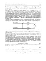
(a) View of the section xy (b) View of the section xz
(c) 3D view
Fig. 1. Schematic drawing and electrodes wiring of a linear electrodynamic trap. The
drawings are not to scale.
acoustic field, equations of motion in the (x,y) plane for a charged particle of mass M and
charge Q, located near the linear trap axis, are:
M
d
2
x
dt
2
= −
Qx
R
2
(U
0
+ V
0

cosΩt) − k
dx
dt
+ F
Ax
(t) (2)
and
M
d
2
y
dt
2
=
Qy
R
2
(U
0
+ V
0
cosΩt) − k
dy
dt
+ F
Ay
(t) (3)
The terms
−k
dx

dt
and −k
dy
dt
, describe the drag force exerted on an object moving in a fluid.
Assuming that the particles are spherical, according to Stokes’s law:
k
= 6πη(d/2) (4)
where d is the diameter of the charged particle while η
≈1.8x10
−5
kgm
−1
s
−1
is the air viscosity
at normal pressure and temperature. The time-depended terms F
Ax
(t) and F
Ay
(t), stand for
the force exerted by the acoustic wave on the stored particle. The Ox is the vertical axis. The
microparticles weight has been neglected. Making change of variable ξ
= Ωt/2 the equations
(2) and (3) can be rewritten as:
d
2
x
dξ
2

+ δ
dx
dξ
+(a
x
+ 2q
x
cos2ξ)x −s
Ax
= 0 (5)
243
Studies on the Interaction Between an Acoustic Wave and Levitated Microparticles
4 Will-be-set-by-IN-TECH
Fig. 2. Microparticles cloud stored along the longitudinal axis of the linear trap
and
d
2
y
dξ
2
+ δ
dy
dξ
+(a
y
+ 2q
y
cos2ξ)y − s
Ay
= 0 (6)

The dimensionless parameters a
x,y
, q
x,y
and δ are given by:
a
x
= −a
y
=
4QU
0
MΩ
2
R
2
(7)
q
x
= −q
y
=
2QV
0
MΩ
2
R
2
(8)
δ

=
6πηd
MΩ
(9)
The time dependent functions s
Ax
(t) and s
Ay
(t) are given by:
s
Ax
(t)=
4F
Ax
MΩ
2
(10)
s
Ay
(t)=
4F
Ay
MΩ
2
(11)
The pair
(a, q) defines the operating point of the electrodynamic trap and determines entirely
the characteristics of the particle motion. In the absence of the terms due to the drag force
(
−k

dx
dt
and −k
dy
dt
) and the acoustic wave F
Ax
(t) and F
Ay
(t), a differential equation of type
(5) or (6) is called the Mathieu equation (McLachlan, 1947). It can be shown that solutions
of a Mathieu equation describe a spatial bounded motion (stable solutions) only for certain
regions of the (a,q) plane called stability domains. This means that, a charged particle can
remain indefinitely in the space between the trap electrodes. Additionally, the charged particle
trajectory must not cross the electrodes surface implying the supplementary restrictions in its
initial position and velocity. One could say that, within the stability domains, a potential
244
Waves in Fluids and Solids
Studies on the Interaction Between an Acoustic
Wave and Levitated Microparticles 5
barrier arises preventing the stored charged particles to escape out of the trap. As an example,
for the first stability domain, if a
x
= 0, the stable solutions are obtained if 0 < q
x
< 0.908.
The first domain stability corresponds to the lowest voltages applied to the trap electrodes.
Due to the air drag area of the first stability domain is enlarged so that, depending on the
value of δ, the particle can remain inside the trap even if q
x

> 0.908. Operation within the
higher order stability domains is not practical because of very high voltage to be applied
across the trap electrodes. As can be seen in (7) and (8) the operating point depends on the
electrodynamic trap geometry, electrodes supply voltages characteristics and charge-to-mass
ratio of the stored particle. Knowing the operating point of the trap, its dimensions and
applied voltages, then charge-to-mass ratio of the stored particle can be estimated. If δ
=
0, F
Ax,y
= 0, |a
x
|, |a
y
|, |q
x
|, |q
y
|1(adiabatic approximation), the differential equations (5) and
(6) have the solutions (Major et al., 2005):
x
(t)=x
0
cos(ω
x
t + ϕ
x
)(1 +
q
x
2

cosΩt
) (12)
y
(t)=y
0
cos(ω
y
t + ϕ
y
)(1 +
q
y
2
cosΩt
) (13)
where
ω
x
=
Ω
2

q
2
x
2
+ a
x
(14)
and

ω
y
=
Ω
2

q
2
y
2
+ a
y
(15)
Under these conditions the motion of a charged particle confined in a quadrupole trap can
be decomposed in a harmonic oscillation at frequencies ω
i
/2π called "secular motion" and a
harmonic oscillation at the frequency f
0
= Ω/2π of ac voltage called "micromotion" . As a
consequence the motional spectrum of the stored particle contains components ω
i
/2π and
f
0
± ω
i
/2π(i = x, y) . For arbitrary values of the parameters a
x,y
, q

x,y
and δ, equations (5) or
(6) can be numerically solved.
3. Experimental setup
The experimental setup is based on the method described in (Schlemmer et al., 2001) used for
a linear trap. The scheme of the experiment is shown in Fig.3. The output beam of a low power
laser module (650 nm, 5 mW) is directed along the longitudinal axis (Oz axis) of the linear trap.
A hole drilled through one of the end-cap electrode (E6) allows the laser beam illuminating
the axial region of the trap where the stored particles density is maximal and the electric
potential is well approximated by the relation (1). A photodetector PD placed outside of the
trap and oriented normal to the laser beam receives a fraction of the radiation scattered by
the stored particles and converts it into an electrical voltage U
ph
proportional to the incident
radiation intensity. To prevent electrical perturbations due to the existing ac high voltage
applied to the electrodes trap, the photodetector is encapsulated in a cylindrical shielding box.
The effect of the background light is removed by means of an appropriate electronic circuit.
The acoustic excitation of the stored microparticles is achieved by a loudspeaker placed next
to the trap. The loudspeaker generates a monochromatic acoustic wave with frequency f
A
.In
this way both electrical field created by the trap electrodes and the force due to the acoustic
wave act simultaneously on the stored microparticles. The motion of the stored particles
245
Studies on the Interaction Between an Acoustic Wave and Levitated Microparticles
6 Will-be-set-by-IN-TECH
Fig. 3. Schematic of the experimental setup
Fig. 4. Block diagram of the measurement chain. The trap electrodes wiring is not shown.
modulates the intensity of the scattered radiation. Therefore the photodetector output voltage
U

ph
contains the same harmonic components. By analysing changes in the structure of the
frequency domain spectrum of the voltage U
ph
, the effect of the acoustic wave on the stored
particles can be evaluated. For this purpose a measurement chain whose block diagram is
shown in Fig. 4 has been implemented. A digital low frequency spectrum analyser is used to
determine the harmonic components of the voltage U
ph
. The loudspeaker is supplied by the
low frequency power amplifier A1 which is driven by the low frequency oscillator O1. The
intensity of the acoustic wave is monitored by means of a sound level meter. Both frequency
and intensity of the acoustic wave can be varied. A similar version of the experimental
setup has been previously described in (Stoican et al., 2008) where preliminary investigations
regarding the effect of the acoustic waves on the properties of the microparticles stored in a
linear electrodynamic trap particle has been reported.
4. Experimental measurements
The microparticles consist of Al
2
O
3
powder, 60-200 μm in diameter, stored at normal pressure
and temperature. The working parameters (U
x
, U
z
and V
0
) of the linear trap were chosen
so that the magnitude of the harmonic component of the photodetector output voltage U

ph
246
Waves in Fluids and Solids
Studies on the Interaction Between an Acoustic
Wave and Levitated Microparticles 7
corresponding to f
0
to reach a maximum (Fig. 5a). This operating point of the trap is known
as "spring point" (Davis et al., 1990). Two typical spectra of the voltage U
ph
recorded in these
experimental conditions are shown in Fig. 6. Only frequencies less than, or equal to 3 f
0
/2,
(a) No acoustic excitation (b) Acoustic excitation, f
A
=75Hz. The
voltage U
ph
appears to be amplitude
modulated.
Fig. 5. Oscilloscope image representing the time variation of the photodetector voltage
output U
ph
in the absence (a) and presence (b) of the acoustic excitation. Experimental
conditions: V
0
=3.3kV, U
x
=0, U

z
=920V, f
0
=80Hz. Experimental results.
(a) U
z
=920V (b) U
z
=100V
Fig. 6. Typical spectra of the photodetector output voltage U
ph
without the acoustic
excitation. Experimental conditions: f
0
=80Hz, V
0
=3.3kV, U
x
=0V. Experimental results.
have been considered because upper lines could be caused by the ac voltage V
ac
waveform
imperfections or digital data processing. Also it was necessary to limit the frequency band
to keep a satisfactory resolution of the recordings. As it can be seen from Fig. 6, under
these conditions, without the acoustic excitation, the spectra of the photodetector output
voltage contain only three significant lines, namely f
0
/2, f
0
and 3 f

0
/2 (here 40Hz, 80Hz and
120Hz). Depending on the applied dc voltages and photodetector position some lines could
missing. Several spectra of the photodetector output voltage U
ph
recorded during acoustic
excitation of the microparticles at different frequencies f
A
are shown in Fig. 7. The measured
sound level was about 85dB. By examining the experimental records, it can be seen that the
supplementary lines occur in the motional spectrum of the stored particles. As an empirical
rule, the frequency peaks due to the acoustic excitation belong to the combinations of the form
f
0
±|f
0
− f
A
|and n|f
0
− f
A
|where n=0, 1, 2 , f
A
is the frequency of the acoustic field and f
0
is
247
Studies on the Interaction Between an Acoustic Wave and Levitated Microparticles
8 Will-be-set-by-IN-TECH

the frequency of the applied ac voltage V
ac
. The rule is valid both for f
A
< f
0
and f
A
> f
0
.As
seen in Fig. 7a and Fig. 7d, the two spectra are almost identical because
|f
0
− f
A
|=20Hz in both
cases. If f
A
is close to the f
0
the lowest frequency component |f
0
− f
A
| yields an amplitude
modulation of the voltage U
ph
very clearly defined (Fig. 5b). The effect is similar to the beat
signal due to the interference of two harmonic signals of slightly different frequencies.

(a) f
A
=60Hz (b) f
A
=67Hz
(c) f
A
=75Hz (d) f
A
=100Hz
Fig. 7. Spectrum of the photodetector output voltage U
ph
when the stored microparticles are
excited by an acoustic wave at different frequencies f
A
. Experimental conditions: f
0
=80Hz,
V
0
=3.3kV, U
x
=0V, U
z
=920V, sound level ≈ 85dB. Experimental results.
5. Numerical analysis of the stored particle motion in an acoustic field
A qualitative interpretation of the experimental results requires a numerical analysis on the
motion of the stored particles. For this purpose the differential equations (5) and (6) must be
numerically solved. Consequently, it is necessary to express functions s
Ax

(t) and s
Ay
(t) from
(10) and (11) in terms of quantities which are known or can be experimentally measured. A
body subjected to an acoustic wave field, experiences a steady force called acoustic radiation
pressure and a time varying force caused by the periodic variation of the pressure in the
surrounding fluid. The radiation pressure is always repulsive meaning that it is directed as
the wave vector. The time varying force oscillates at the frequency of the acoustic wave and its
time average is equal to zero. The radiation pressure
F
R
exerted on a rigid spherical particle
by a plane progressive wave is derived in (King, 1934) as:
F
R
=
π
5
d
6
λ
4
wF(ρ
0
/ρ
1
) (16)
248
Waves in Fluids and Solids
Studies on the Interaction Between an Acoustic

Wave and Levitated Microparticles 9
where d is the particle diameter, λ is the wavelength of the acoustic wave and w represents the
acoustic energy density. The parameter F
(ρ
0
/ρ
1
) is called relative density factor being given by:
F
(ρ
0
/ρ
1
)=
1 +
2
9
(1 − ρ
0
/ρ
1
)
2
(2 + ρ
0
/ρ
1
)
2
(17)

where ρ
0
and ρ
1
are air and particle density, respectively. If ρ
0
/ρ
1
1, as in the present
case (see bellow), practically F
(ρ
0
/ρ
1
)=0.305. For a plane progressive acoustic wave, energy
density is (Beranek, 1993; Kinsler et al., 2000):
w = p
2
s
/ρ
0
c
2
(18)
where p
s
is sound pressure and c is the speed of propagation of the acoustic wave. Sound
pressure can be estimated according to the formula which defines the sound pressure level SPL:
SPL
= 20log

10
p
s
p
re f
(19)
where p
re f
=2x10
−5
N/m
2
is the standard reference pressure. Sound pressure level (SPL) is
expressed in dB and can be experimentally measured by using sound level meters. In (King,
1934), as an intermediate result, the velocity of a spherical particle placed in an acoustic wave
field is given as:
dr
dt
= −
A
1
α
3
k
0
ρ
0
ρ
1
1

F
1
−iG
1
(20)
where k
0
= ω/c, α = k
0
d/2, while ω = 2π f
A
is the angular frequency of the acoustic wave. If
ρ
0
/ρ
1
1 and α  1 then F
1
(α)  2/α
3
and G
1
(α) −1/3. The quantity A
1
is a measure of
wave intensity. Assuming a monochromatic plane progressive acoustic wave, the amplitude
of the acoustic oscillating force exerted on the particle may be written:
F
A0r
= |M

d
2
r
dt
2
| =
ωM|A
1
|
α
3
k
0
ρ
0
ρ
1
1
|F
1
−iG
1
|
(21)
where
|A
1
| = 3cv/ω. Taking into account expressions for F
1
, G

1
, |A
1
|, α and k
0
, written above,
the relation (21) becomes:
F
A0r
= 2ωMv
ρ
0
ρ
1
(22)
The quantity v represents the amplitude of the velocity of the surrounding fluid particles
(air in this case), which are oscillating due to the acoustic wave, and is related to the sound
pressure by the relation:
v
=
√
2p
s
ρ
0
c
(23)
Finally, the amplitude of the oscillating force, considering ρ
0
/ρ

1
1 and α  1, is:
F
A0r
=
2
√
2ωMp
s
ρ
1
c
(24)
Consequently:
F
Ar
= F
R
+ F
A0r
cos(2π f
A
t + β) (25)
249
Studies on the Interaction Between an Acoustic Wave and Levitated Microparticles
10 Will-be-set-by-IN-TECH
As further numerical evaluations will demonstrate the acoustic radiation pressure F
R
is
several order of magnitude less than that of oscillating force amplitude F

A0r
and has been
neglected. In order to simplify theoretical analysis, the weight of the microparticles (i. e.
Mg where g=9.8m/s
2
) has been also neglected. Experimentally, the microparticles weight are
usually compensated by the electric field due to the dc voltage U
x
. As a result, considering
the experiment geometry (Fig. 4):
F
Ax
(t)=F
Ay
(t) ≈
√
2
2
F
A0r
cos(2π f
A
t + β) (26)
Therefore the two function s
Ax
(t) and s
Ay
(t) takes form:
s
Ax

(t)=s
Ay
(t)=s
A0
cos(2π f
A
t + β)=s
A0
cos(2
f
A
f
0
ξ + β) (27)
where
s
A0
=
8ωp
s
ρ
1
cΩ
2
(28)
All quantities existing in formula (28) are known or can be experimentally measured.
The operating conditions considered for numerical analysis are summarized in Table 2 .
The diameter of the Al
2
O

3
microparticles can vary in the range from 60μmto200μm, as
Parameter Notation Value
trap inner radius R 5x10
−3
m
particle density (Al
2
O
3
) ρ
1
3700 kg/m
3
air density ρ
0
1.2 kg/m
3
speed of sound c 343 m/s
air viscosity η 1.8x10
−5
kgm
−1
s
−1
sound pressure level SPL 85 dB
sound pressure p
s
0.35 N/m
2

sound frequency f
A
100 Hz
ac voltage frequency f
0
80 Hz
Table 2. Operating conditions considered for numerical analysis
before mentioned. The two corresponding limit values of the parameters depending on the
microparticles size, are shown in Table 3. The operating conditions taken into account are the
same as in Table 2. According to numerical values listed in Table 2 and Table 3, ρ
0
/ρ1 1 and
particle diameter d 6x10
−5
m 2x10
−4
m
particle mass M 4.18 x 10
−10
kg 1.55 x 10
−8
kg
particle weight Mg 4.10 x 10
−9
N 1.51 x 10
−7
N
α
= k
0

d/2 5.49 x 10
−5
1.83 x 10
−4
δ 0.09 0.008
acoustic radiation pressure
F
R
2.82 x 10
−32
N 3.87 x 10
−29
N
oscillating force amplitude F
A0r
2.08 x 10
−13
N 7.71 x 10
−12
N
s
A0
/R 1.11 x 10
−6
1.11 x 10
−6
Table 3. The limit values corresponding to the particle possible diameter. Operating
conditions are listed in Table 2
250
Waves in Fluids and Solids

Studies on the Interaction Between an Acoustic
Wave and Levitated Microparticles 11
α 1, which are in good agreement with our previous assumptions. Fourier transforms X( f )
and R( f ), of the rectangular x(t) and radial r(t)=

x
2
(t)+y
2
(t) coordinates, respectively,
in the range from 0 to 125Hz, without the acoustic excitation, obtained by solving numerically
differential equations (5) or (6), for several values of the parameters q
x
, are shown in Fig.8.
Fourier transforms of x
(t) and y(t) are similar. As theory of Mathieu equations ascertains,
numerical calculations shows that for
|q
x,y
|1, the motional spectrum contains mainly
harmonic components due to the secular motion, namely ω
x
/2π and f
0
±ω
x
/2π. In practice,
the microparticles trapping in such conditions is difficult to be achieved because the potential
barrier is too low so that weak external perturbations can eject stored particles out of the
trap. The numerical results show that, close to the limit of the first stability domain, the

micromotion becomes important and the motional spectrum contains only a few significant
lines, namely at f
0
for r(t) and at f
0
/2 and 3 f
0
/2 for x(t), respectively. Fourier transforms
X
( f ) and R( f ), of the rectangular x(t) and radial r(t) coordinates, respectively, in the range
from 0 to 125Hz, in the presence of the acoustic excitation, obtained by solving numerically
differential equations (5) or (6), for several values of the acoustic wave frequency f
A
,are
shown in Fig. 9. Simulation conditions are listed in Table 4. Expression of the parameter
s
A0
/R corresponds to SLP=85dB and R=5mm. All the remaining parameters, except acoustic
wave frequency f
A
, are listed in Table 2 and Table 3 The variation of the normalized time
f
0
[Hz] q
x
a
x
δ s
A0
/R r(0)

˙
r
(0) β time interval[s]
80 0.908 0 0.01 0.11 x 10
−7
f
A
[Hz] 0 0 0 0-40
Table 4. Conditions taken into account to simulate the motion of the a microparticle in the
presence of an acoustic field (Figs.9 and 10)
average,
r(t)/R, of the coordinate r as a function of acoustic wave frequency f
A
is shown
in Fig 10. As on can see from this figure there are two critical frequencies of the acoustic
wave, namely f
0
/2 and 3 f
0
/2, where the amplitude of the particle motion rises sharply. It is
interesting to note that this very high growth of the motion amplitude does not occur for
f
A
= f
0
. The microparticles cloud appears to form a non-linear oscillating system for which
resonance frequencies occur at pf
0
/q with p and q integer (Landau & Lifshitz, 1976).
The variation of the normalized time average,

r(t)/R, of the coordinate r as a function of
log
10
(s
A0
/R) at acoustic wave frequency f
A
=120Hz is shown in Fig 11. According to (28)
and (19) the parameter s
A0
may be considered a measure of the acoustic excitation because
log
10
(s
A0
)=log
10
p
s
+ constant and sound pressure level SPL depends on log
10
p
s
.Ason
can see from this figure, beyond a threshold value, the average distance from the trap axis
grows monotonically with the level of the sound pressure level. Around s
A0
/R  10
−8
there

is a threshold value where amplitude of the microparticle motion increases suddenly (the
region within the green frame from Fig.11). The transition is not uniform, there are maximum
and minimum values of
r(t). This phenomenon could be interpreted as so called collapse of
resonance which means that the amplitude of resonance goes to zero for some value of the
perturbation amplitude (Olvera, 2001). However numerical result must be regarded with
caution. Some hypothesis aimed to simplify mathematical treatment has been introduced. For
example it was assumed that the parameter β is equal to zero and it remains constant. In fact
β, which signifies the phase shift between ac voltage V
ac
and acoustic wave, varies randomly
because the two oscillations are produced by different generators. Further experiments are
necessary to confirm theoretical assertions. All of the numerical results have been obtained by
using SCILAB 5.3.1.
251
Studies on the Interaction Between an Acoustic Wave and Levitated Microparticles
12 Will-be-set-by-IN-TECH
(a) q
x
=0.1 (b) q
x
=0.5
(c) q
x
=0.9 (d) q
x
=0.908
Fig. 8. X
n
( f )=X( f )/X

max
( f ) (red) and R
n
( f )=R( f )/R
max
( f ) (blue) where X( f ) and R( f )
are Fourier transform of the rectangular x(t) and radial r(t) coordinates, respectively, for
0< f <125Hz, a
x
=0, f
0
= Ω/2π=80Hz, δ=0.01, without the acoustic excitation. Numerical
result.
252
Waves in Fluids and Solids
Studies on the Interaction Between an Acoustic
Wave and Levitated Microparticles 13
(a) f
A
=60Hz (b) f
A
=67Hz
(c) f
A
=75Hz (d) f
A
=100Hz
Fig. 9. X
n
( f )=X( f )/X

max
( f ) (red) and R
n
( f )=R( f )/R
max
( f ) (blue) where X( f ) and R( f )
are Fourier transform of the rectangular x(t) and radial r(t) coordinates, respectively, for
0< f <125Hz, in the presence of the acoustic excitation, for several values of the acoustic wave
frequency f
A
. The plots correspond to the frequency f
0
=80Hz of the ac supply voltage V
ac
and to an incident sound level of 85dB. A complete list of the simulation conditions is
displayed in Table 4. Numerical result.
253
Studies on the Interaction Between an Acoustic Wave and Levitated Microparticles
14 Will-be-set-by-IN-TECH
Fig. 10. The normalized time average of the coordinate r(t) as a function of acoustic wave
frequency f
A
. R represents the inner radius of the linear trap. Simulation conditions are
displayed in Table 4. Numerical result.
(a) Complete view (b) Expanded view of the region within
the green frame
Fig. 11. The normalized time average of the coordinate r(t) as a function of parameter s
A0
/R
at acoustic wave frequency f

A
=120Hz. Parameter s
A0
is a measure of acoustic
excitation(log
10
(s
A0
) ∼ SP L). Simulation conditions, except parameter s
A0
/R, are displayed
in Table 4. Numerical result.
6. Conclusion
Although measurements result has been interpreted using an approximative and simplified
theory of the linear trap, by comparing the experimental spectra with numerical simulations
a good qualitative agreement can be noticed. The spectrum of the laser radiation intensity
scattered by the stored microparticles seems to be a superposition of the r
(t) and x(t) (or y(t))
harmonic components, respectively. Because the experimental spectrum obtained without
the acoustic excitation, shown in Fig.6 is similar to that displayed in Fig.8d we may suppose
that operating point of the linear trap during the experiment corresponds to q
x
≈ 0.908 (i.e.
Q/M
≈5.4 x 10
−4
C/kg cf. (8)). The simulation of the stored particle motion in an acoustic
wave has been done taking into account this assumption. By knowing the ratio Q/M and
the mass of a microparticle (from Table 3) electric charge Q can be evaluated. Because the
microparticles are stored in air at normal pressure, a supplementary restriction on the physical

characteristics of the microparticles arises. Assuming that microparticles are spherical and the
254
Waves in Fluids and Solids
Studies on the Interaction Between an Acoustic
Wave and Levitated Microparticles 15
electric charge is uniform distributed over its surface, the electric field E
d
at the surface is:
E
d
=
Q
4π
0
(d/2)
2
(29)
where 
0
=8.854 x 10
−12
F/m. Electric charge Q results from:
Q
= M(
Q
M
)=
4π
3
(

d
2
)
3
ρ
1
(
Q
M
) (30)
where Q/M is known. The electric field E
d
can not exceed a certain threshold value E
max
,
called dielectric strength, at which surrounding gas molecules become ionized, so that the
condition E
d
< E
max
is necessary. From (29) and (30), the above condition can be written:
d
<
6
0
E
max
(Q/M)ρ
1
(31)

The dielectric strength E
max
varies with the shape and size of the charged body, humidity
and pressure of the air. We consider here the dielectric strength of air E
max
≈3x10
6
V/m.
By replacing numerical values in (31), it results that d<69μm. Therefore the diameter of the
microparticles which produce the laser beam scattering sensed by the photodetector lies in the
range 60-69μm. Distribution of the frequency peaks are almost identical both in experimental
recordings and numerical simulation, but their relative heights are different. Besides a
simplified theoretical approach, there are a few possible experimental issues. The dc voltages
U
x
and U
z
shift the stored microparticles cloud position relative to the trap axis and, implicitly,
to the photodetector aperture. Thus, viewing angle of the photodetector is modified and
some harmonic components could not be observed or appear to be very weak. On the other
hand, non-uniformity of the frequency characteristic for the common loudspeakers, especially
at frequencies below 100Hz, could distort experimental recordings. Numerical estimations
demonstrate that, in the described experimental conditions and within the considered range
of the acoustic wave frequency, the acoustic radiation pressure
F
R
is very weak compared
to the microparticles weight Mg or amplitude of the oscillating force exerted by acoustic
wave F
A0r

(see Table 3). Certainly, the first improvement of theoretical approach would be
to add a constant term corresponding to the microparticles weights in differential equations
(2) and/or (3), depending on the orientation of the reference system. Like weight, acoustic
radiation pressure does not vary in time and can be regarded, mathematically speaking, as
a small correction of the microparticles weight. As a result the acoustic radiation pressure is
not important here, where only acoustic waves with frequency around frequency f
0
of the ac
voltage have been investigated. The acoustic radiation pressure can become significantly at
higher frequencies, (see (16)) varying according to f
4
. On the other hand, according to the
numerical results, if the intensity of the acoustic wave is larger than a threshold value and
its frequency has proper values, the amplitude of the stored microparticles motion increases
significantly. These frequencies are identical to certain frequency peaks existing in the
motional spectrum of the stored particle predicted by the numerical simulations (Fig. 8d) and
observed experimentally (Fig.6b). Therefore its action is effective only for the microparticles
species whose properties meet certain conditions. In this way, theoretically, the selective
manipulation of the stored microparticles by means of the acoustic waves becomes possible.
We gratefully acknowledge material support provided by Mira Technologies Group SRL -
Bucharest, Romania.
255
Studies on the Interaction Between an Acoustic Wave and Levitated Microparticles
16 Will-be-set-by-IN-TECH
7. References
Beranek, L. L. (1993). Acoustics, Acoustical Society of America, New York.
Carleton, K. L., Sonnenfroh, D. M., Rawlins, W. T., Wyslouzil, B. E. & Arnold, S. (1997).
Freezing behavior of single sulfuric acid aerosols suspended in a quadrupole trap,
Journal of Geophysical Research Vol. 102(No. D5): 6025–6033.
Davis, E. J. (1997). A history of single aerosol particle levitation, Aerosol Science and Technology

Vol. 26(No. 3): 212–254.
Davis, E. J., Buehler, M. F. & Ward, L. T. (1990). The double-ring electrodynamic balance for
microparticle characterization,Review of Scientific Instrument Vol.61(No. 4): 1281–1288.
Gheorghe, V. N., Giurgiu, L., Stoican, O., Cacicovschi, D., Molnar, R. & Mihalcea, B. (1998).
Ordered structures in a variable length a.c. trap., Acta Physica Polonica A Vol.93(No.
4): 625– 629.
Jakubczyk, D., Zientara, M., Bazhan, W., Kolwas, M. & Kolwas, K. (2001). A device
for light scatterometry on single levitated droplets, Opto-Electronics Review Vol.
9(No.4): 423–430.
King, V. L. (1934). On the acoustic radiation pressure on spheres, Proceedings of the Royal Society
(London) Vol.A147: 212–240.
Kinsler, L. E., Frey, A. R., Coppens, A. B. & Sanders, J. V. (2000). Fundamentals of Acoustics,
John Wiley and Sons, Inc, New York.
Landau, L. D. & Lifshitz, E. M. (1976). Mechanics, Butterworth-Heinemann, Oxford.
Major, F. G., Gheorghe, V. N. & Werth, G. (2005). Charged Particle Traps, Physics and Techniques
of Charged Particle Confinement, Springer, Berlin Heidelberg New York.
March, R. E. (1997). An introduction to quadrupole ion trap mass spectrometry, Journal of Mass
Spectrometry Vol. 32: 351–369.
McLachlan, N. W. (1947). Theory and Application of Mathieu Functions, Clarendon Press, Oxford.
Olvera, A. (2001). Estimation of the amplitude of resonance in the general standard map,
Experimental Mathematics Vol.10(No. 3): 401–418.
Pedregosa, J., Champenois, C., Houssin, M. & Knoop, M. (2010). Anharmonic contributions in
real rf linear quadrupole traps, International Journal of Mass Spectrometry Vol. 290(No.
2-3): 100–105.
Peng, W. P., Yang, Y. C., Kang, M. W., Lee, Y. T. & Chang, H. C. (2004). Measuring masses
of single bacterial whole cells with a quadrupole ion trap, Journal of the American
Chemical Society Vol. 126(No.38): 11766–11767.
Schlemmer, S., Illemann, J., Wellert, S. & Gerlich, D. (2001). Nondestructive high-resolution
and absolute mass determination of single charged particles in a three-dimensional
quadrupole trap, Journal of Applied Physics Vol. 90(No. 10): 5410–5418.

Shaw, R. A., Lamb, D. & Moyle, A. M. (2000). An electrodynamic levitation system for
studying individual cloud particles under upper-tropospheric conditions, Journal of
Atmospheric and Oceanic Technology Vol. 17(No. 7): 940–948.
Stoican, O. S., Dinca, L. C., Visan, G. & Radan, S. (2008). Acoustic detection of the
parametrical resonance effect for a one-component microplasma consisting of the
charged microparticles stored in the electrodynamic traps, Journal of Optoelectronics
and Advanced Materials Vol.10(No. 8): 1988–1990.
Stoican, O. S., Mihalcea, B. & Gheorghe, V. N. (2001). Miniaturized microparticle trapping
setup with variable frequency, Roumanian Reports in Physics Vol. 53(No. 3-8): 275–280.
Wuerker, R. F., Shelton, H. & Langmuir, R. V. (1959). Electrodynamic containement of charged
particles, Journal of Applied Physics Vol. 30(No. 3): 342–349.
256
Waves in Fluids and Solids
10
Acoustic Waves in Bubbly Soft Media
Bin Liang
1
, Ying Yuan
2
, Xin-ye Zou
1
and Jian-chun Cheng
1

1
Nanjing University, Nanjing
2
Jiangsu Teachers University of Techonology, Changzhou
P. R. China
1. Introduction

There exists a special class of solid media called soft media (or weakly compressible media),
for which the inequality λ>>μ is satisfied (λ and μ are the Lamé coefficients) [1-6]. Such
media with very small shear stiffness are dynamically similar to liquids to a great extent and
exhibit strongly a “water-like” characteristic and, therefore, are also associated with the
name of “water-like” media. The class of soft media includes many common media in the
fields of scientific research and practical applications (e.g. soft rubbers, tissues, or
biomimetic materials), and air bubbles are often introduced due to artificial or non-artificial
reasons. In the presence of air bubbles in a soft medium, the bubbles will oscillate violently
as an acoustic wave propagates in the bubbly medium. It has been proved that only if the
ratio λ>>μ is sufficiently large can a bubble in a solid behave like an oscillator with a large
quality factor, otherwise oscillation will be damped within a short time comparable to its
period [7]. This results in the fact that the acoustical property of a bubbly soft medium is
particularly different from that of a usual solid medium containing bubbles. The strong
scattering of acoustic waves by bubbles in soft media may lead to some significant physical
phenomena stemming from the multiple-scattering effects, such as the localization
phenomenon [8-11]. On the other hands, a bubbly soft medium has potential applications to
a variety of important situations, such as the fabrication of acoustic absorbent with high
efficiency or the clinic application of ultrasonic imaging utilizing the contrast agents [12].
Consequently, it is of academic as well as practical significance to make a comprehensive
study on the acoustic waves in a bubbly soft medium.
Attempts to theoretically investigate the bubble dynamics in a soft medium go back many
decades [1-4]. Meyer et al have performed the early measurements of the resonance
frequency of a bubble in rubbers [1]. The dynamical equation for arbitrarily large radial
motion has been derived by Erigen and Suhubi in Rayleigh-Plesset form [2]. Ostrovsky has
derived a Rayleigh-Plesset-like equation to describe the nonlinear oscillation of an
individual bubble in a soft medium [3,4]. On the basis of the linear solution of the bubble
dynamic equation of Ostrovsky, Liang and Cheng have theoretically investigated the
acoustic propagation in an elastic soft medium containing a finite number of bubbles [8-11].
By rigorously solving the wave field using a multiple-scattering method, they have revealed
the ubiquitous existence of the significant phenomenon of acoustic localization in such a

class of media, and identified the “phase transition” phenomenon similar with the order-
disorder phase transition in a ferromagnet. For practical samples of bubbly soft media,
however, the multiple-scattering method usually fails due to the extremely large number of

Waves in Fluids and Solids

258
bubbles and the strong acoustical nonlinearity in such media. In such cases, a more useful
approach is to treat the bubbly soft media as a homogeneous “effective” medium
characterized by nonlinear effective parameters, which are remarkably influenced by many
factors associated with bubble oscillations such as surface tension, compressibility, viscosity,
surrounding pressure, and an encapsulating elastic shell. Emelianov et al have studied the
influence of surrounding pressure on the nonlinear dynamics of a bubble in an
incompressible medium [5]. Their model has then been extended by Zabolotskaya et al to
account for the effects of surface tension, viscosity, weak compressibility, and elastic shell [6].
Based on the bubble dynamics model of Zabolotskaya et al, Liang et al have developed an
effective medium method (EMM) to give description of the nonlinear sound propagation in
bubbly soft media with these effects accurately included [12]. Compared with the viscosity of
soft medium, the resonance of the system introduced by bubbles becomes the most dominant
mechanism for acoustic attenuation in a bubbly soft medium which necessarily depends on
the parameters of bubbles [13].

With the availability of obtaining the effective acoustical
parameters of bubbly soft media, Liang et al have presented an optimization method on the
basis of fuzzy logic and genetic algorithm to yield the optimal acoustic attenuation of such
media by optimizing the parameters of the size distribution of bubbles [14].
The chapter is structured as follows: we first focus on the phenomenon of acoustic
localization in elastic soft media containing finite numbers of bubbles in Section 2. In Section
3, we study the phase transition in acoustic localization which helps to identify the
phenomenon of localization in the presence of viscosity. In Section 4, we discuss the EMM to

describe nonlinear acoustic property of bubbly soft media. Finally in Section 5, we study
how to enhance the acoustic attenuation in soft bubbly media in an optimal manner.
2. Acoustic localization in bubbly soft media
In this section, we theoretically study the sound propagation in an elastic soft medium
containing a finite number of bubbles by using a self-consistent method to reveal the
existence of acoustic localization under proper conditions. It will be proved that the
phenomenon of localization can be identified by properly analyzing the spatial correlation
of wave field.
2.1 The model
Consider a longitudinal wave in an elastic soft medium containing air bubbles with small
volume fraction
β
. We shall restrict our attention to the wave propagation at low
frequencies, i.e.,
0
1kr << . Here /
l
kc
ω
= and (2)/
l
c
λ
μρ
=+ are the wavenumber and
the speed of the longitudinal wave, respectively, and
ρ
is the mass density. The wave is
assumed to be of angular frequency
ω

and emitted from a unit point source located at the
origin, surrounded by N spherical air bubbles that are randomly located at
i
r in a not
overlapping way with
1,2, ,iN=⋅⋅⋅. For simplicity and without loss of generality, all the
bubbles are assumed to be of uniform radius
0
r and randomly distributed within a spatial
domain, which is taken as the spherical shape so as to eliminate irrelevant effects due to an
irregular edge. Then the radius of the spherical bubble cloud is
1/3
00
(/)RN r
β
= . Here the
source is placed inside rather than outside the bubble cloud, which is the only way to isolate
the localization effect from boundary effects and unambiguously investigate the problem of
whether the transmitted waves can indeed be trapped [15].

Acoustic Waves in Bubbly Soft Media

259
2.2 Validation of approximation
As the incident longitudinal wave is scattered by a bubble in soft media, the energy
converted into shear wave can be expected negligible, on condition of sufficiently small
shear stiffness. Next we shall present a numerical demonstration of the validation of such an
approximation by inspecting the scattering cross section of a single bubble in soft media.
The total scattering cross section
σ

of a single bubble can be expressed as
LS
σσ σ
=+
,
where
L
σ
and
S
σ
refer to the contributions of the scattered longitudinal and shear waves,
respectively. Therefore it is conceivable that the ratio
/
LS
σσ
actually reflects the extent to
which the mode conversion will occur as the incident longitudinal wave is scattered by the
bubble. The value of
/
LS
σσ
can be readily obtained from Eq. (19) in Ref. [16].
A series of numerical experiments has been performed for an individual bubble in a variety
of media, for the purpose of investigating how the energy converted into shear wave is
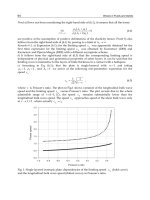
affected as the media of matrix varies. Figure 2.1 presents the typical result of the
comparison between the ratios
/
LS
σσ

versus frequency
0
kr for different media of matrix.
Three particular kinds of elastic soft media are considered: Agar-gelatin, plastisol, and
gelatin. Aluminum is also considered for comparison. The physical parameters of these
materials are listed in Table 2.1. Note that the physical parameters of soft media
approximate to those of water except for different values of shear moduli, which seems to be
natural for such “waterlike” media.
From Fig. 2.1, we find: (1) the energy of the scattered shear wave is extremely small when
compared to that of the scattered longitudinal wave, as long as the ratios /
λ
μ
are
sufficiently large. Contrarily the magnitude of the longitudinal components is nearly the
same to the shear components in the scattered field for
μ
comparable with
λ
. (2) for an
individual bubble in different soft media, the energy converted into shear wave is
diminished as the shear modulus of the medium of matrix decreases, as expected. (3)
moreover, the ratios
/
LS
σσ
are greatly enhanced in the proximity of the natural resonance
of the individual bubbles, owing to the giant monopole resonance that is the dominant
mode of bubble pulsation at low frequencies [17].

Fig. 2.1 The ratio
/
LS
σσ
versus frequency
0
kr
for a single bubble in different materials.

Waves in Fluids and Solids

260
Thereby it follows that the energy converted into shear waves is insignificant as the incident
longitudinal wave is scattered by a bubble in soft media. The shear component of the
scattered field may thus be expected to be negligible as the longitudinal wave propagates in
a bubbly soft medium. It should be stressed, however, that such an approximation can only
be regard valid under the condition that the propagation of the elastic waves is not
completely diffusive. Otherwise there will be an entirely contradicting conclusion that the
ratio between the energy of the shear and the longitudinal wave is as large as
3
2( / )
ls
cc
when the wave field is completely diffusive [18,19]. Here
2/
s
c
μρ
=
is the speed of the

shear wave.
Such a seeming paradox may be clarified by estimating the ratio between the mean free path
(MFP) of the wave and the linear “sample size”
R of the random medium. For a classical
wave propagating in a random media, the transport MFP is defined as the length over
which momentum transfer becomes uncorrelated, while the elastic MFP is the average
distance between two successive scattering events [20].
For an elastic wave, the following inequality has to be fulfilled to completely attain the
diffusive regime [21]:


1/
l
T
kl R<< << , 1/
s
T
lR
κ
<< << ,
where
l
T
l and
s
T
l refer to the transport MFPs of longitudinal wave and shear wave
respectively,
/
s

c
κω
= is the wave number of the shear wave. Otherwise the wave
propagation will be predominantly ballistic as the ratio between the MFP and the sample
size is large [22].
At low frequencies from
0
kr =0 to 0.1, a set of numerical experiments have been carried out
to estimate the MFPs of the elastic waves in various bubbly soft media for all the structure
parameters employed in the present study. The typical values of the sample size
R lie
roughly within the range
4
4 10 m 0.8mR
−
×≤≤. The results indicate that: (1) for the shear
wave in bubbly soft media, the typical values of the transport MFP
s
T
l and the elastic MFP
s
E
l of shear wave lie approximately within the range
35
610m , 410m
ss
TE
ll
−
×≤≤×. For any

particular set of structure parameters, both the transport MFP
s
T
l and the elastic MFP
s
E
l are
much larger than the sample size, i.e., ,
ss
ET
ll R>> . This manifests that the scattering of the
low-frequency shear wave by the bubbles in a soft medium is weak and, therefore, the
propagation of the shear wave in such a medium is ballistic rather than diffusive. (2) for the
longitudinal wave, for most frequencies the range of the typical values of
l
T
l and
l
E
l are
roughly
35
410m , 310m
ll
TE
ll
−
×≤≤× and the relation ,
ll
ET

ll R>> holds for any particular set
of structure parameters, except for a frequency range within which
6
1 10 m 0.8m
l
T
l
−
×≤≤
and the Ioffe-Regel criterion 1
l
T
kl ≤ is satisfied for any particular set of structure parameters
[23].

As will be explained later, such a frequency range is in fact the region where the
phenomenon of acoustic localization occurs. This is consistent with the conclusion regarding
a bubbly liquid that the coherent wave dominates the transmission for most frequencies
except for the localization region [24].
As a result, the condition to attain a completely diffusive wave field can not be satisfied at
low frequencies as the longitudinal wave propagates in a bubbly soft medium.
Consequently, the shear component of the scattered field is unimportant when compared to
the longitudinal component, and neglect of mode conversion only leads to negligible errors.

Acoustic Waves in Bubbly Soft Media

261
The results of the numerical experiments indicate that the numerical error caused by
neglecting mode conversion is less than 1% as long as the ratio
/

λμ
is roughly larger than
4
10 . In the following study, we shall assume the scattered field to be totally longitudinal
without taking mode conversion into consideration.

Materials
ρ
(kg/m
3
)
λ

μ

/
λμ

Agar-gelatin
a
1000 2.25GPa 6.35KPa 4×10
5

plastisol
b
1000 2.55GPa 12.1KPa 2×10
5

gelatin
c

1000 2.25GPa 39.0KPa 5×10
4

aluminum 2700 111.3GPa 37.1GPa 3
a
Reference [25].
b
References [4], [26], and [27].
c
Reference [6].
Table 2.1. The physical parameters of the materials
2.3 The bubble dynamics
For an individual bubble in soft elastic media, the radial pulsation driven by a plane
longitudinal wave is described by a Rayleigh-Plesset-like equation, as follows [3,4]:


2
23 2
22
0
0
23 2
2
inc
l
dU r dU dU dU
UGUqU ep
dt c dt dt dt
ω



+− = + + −





, (2.1)
where
33
0
4( )/3
in
Urr
π
=− is volume perturbation of an individual bubble with
in
r
being the
instantaneous radius,
inc
p
refers to the incident plane wave on the bubble, i.e., the driving
force of the bubble pulsation,
22
012
ωωω
=+ is the bubble resonance frequency with
2
10

4/r
ω
μρ
= and
22
20
3/
aa
cr
ω
ρρ
= corresponding to the Meyer-Brendel-Tamm
resonance and the Minnaert bubble resonance, respectively [8], the parameters of
G ,
q
, and
e are given as
2
0
(9 2 ) /2Gq
χω
=+ ,
3
0
1/(8 )
q
r
π
= ,
0

4/er
π
ρ
=
. Here
χ
is a coefficient of
asymmetry, which must lie in the range 0 1
χ
<≤. For a spherical bubble 1
χ
= . Up to the
first order approximation, one obtains the harmonic solution of Eq. (2.1), as follows

0
22 3
00
4
,
(/)
inc
l
r
Up
ir c
π
ρω ω ω
=−
−−
(2.2)

At low frequencies, the acoustic field produced by acoustic radiation from a single bubble is
taken to be the diverging spherical wave [6]

2
2
1
(,) ()exp( )
4
ss
l
dr
ptp it Ut
rdt c
ω
π

=−≈− −


rr
, (2.3)

We assume that the bubble is the i th bubble located at
i
r and express the incident plane
wave as

(,) ()exp( )
inc inc
p

tp it
ω
=−rr , (2.4)

Waves in Fluids and Solids

262
Substituting Eqs. (2.2) and (2.4) in Eq. (2.3) and discarding the time factor exp( )it
ω
− , one
obtains the scattered wave at
r from the i th bubble, denoted by ( )
i
s
p r , as follows:


0
() ( ) ( )
i
sinci i
pfpG=−rrrr, (2.5)
where
0
()exp(||)/||
iii
Gik−= − −rr rr rr is the usual three-dimensional Green’s function,
f

is the scattering function of a single bubble, defined as

0
22
00
(/ 1 )
r
f
ikr
ωω
=
−−
, (2.6)
Eqs. (2.5) and (2.6) clearly show that the scattered fields and scattering function of a single
bubble in soft media take an identical form as in liquid media, except for different
expressions of
0
ω
(see Eqs. (2) and (2) in Ref. [24] and also Eq. (2) in Ref. [28]). Compared
with the resonance frequency of a bubble in liquid media that includes only the Minnaert
contribution
2
ω
, an additional term
1
ω
is present in Eq. (2.6), due to the contribution of
shear wave in the solid wall of bubble. In the limiting case /
λ
μ
→∞, the soft medium

becomes a liquid medium, and Eq. (2.6) degenerates to Eq. (4) in Ref. [24] due to the
vanishing of
1
ω
. Despite such an agreement of the results in the form, we have to
particularly stress that it is the radial pulsation equation of a single bubble from which the
present theory begins, rather than the well-studied scattering function of a bubble employed
in Ref. [24].
2.4 The self-consistent formalism
Among many useful formalisms suggested for describing the acoustic scattering by a finite
group of random scatterers, the self-consistent method is proved to be particularly effective
[29]. This method is based on a genuine self-consistent scheme proposed first by Foldy [30]
and reviewed in Ref. [31]. Later Ye et al employed the self-consistent method to investigate
the wave propagation in a bubble liquid [24]. In the method, the multiple scattering of
waves is represented by a set of coupled equations, and the rigorous results can be obtained
by solving the equations. In the present study, the wave propagation in a bubbly soft
medium will be solved by using the self-consistent method in an exact manner.
In the presence of bubbles, the radiated wave from the source is subject to multiple
scattering by the surrounding bubbles. Hence the total acoustic wave at a spatial point
r is
supposed to include the contributions from the wave directed from the source and the
scattered waves from all bubbles, i.e.,

0
1
() () ()
N
i
s
i

pp p
=
=+

rr r, (2.7)
Analogously, the incident wave upon the i th bubble should consist of the direct wave from
the source and the scattered waves from all bubbles except for itself, i.e., [31]

0
1,
() () ()
N
j
inc i i s i
jji
pp p
=≠
=+

rr r, (2.8)

Acoustic Waves in Bubbly Soft Media

263
At
0
1kr << , the dimension of bubbles is very small when compared to the wavelength, and
the plane wave approximation still stands for the incident wave upon an individual bubble.
In this situation, the dynamics of an individual bubble can be described by the radial
pulsation equation given by Eq. (2.1). Therefore for the i th bubble, according to Eqs. (2.5)

and (2.8), the following self-consistent equation should be satisfied:

00
1,
() () () ( )
N
j
i
sisii
jji
pfp pG
=≠

=+ −




rr rrr
, (2.9)

Upon incidence, each bubble acts effectively as a secondary pulsating source. The scattered
wave from the i th bubble is regarded as the radiated wave and is rewritten as

[28]

0
() ( )
i
si i

pAG=−rrr (2.10)
where the complex coefficient
i
A
refers to the effective strength of the secondary source.
Substitution of Eq. (2.10) in Eq. (2.8) yields

00
1,
() ( )
N
ii jji
jji
Afp AG
=≠


=+ −





rrr
, (2.11)

By setting r in Eq. (2.10) to any bubble other than the i th, this equation becomes a set of
closed self-consistent equations which can be expressed as

f

=+APCA
, (2.12)
where
[]
12
, , ,
T
N
AA A=A ,
[]
01 02 0
( ), ( ), , ( )
T
N
pp p= rr rP , C is an NN× matrix, defined as
11 1
1
N
NNN
CC
CC




=







C



,
where
0
(1 ) ( )
i
j
i
jj
i
CfG
δ
=− −rr with
i
j
δ
being the Kronecker symbol. It is apparent that C is
symmetric according to the principle of reciprocity. One may readily obtain from Eq. (2.12)

1
(1 )f
−
=−ACP
. (2.13)
For an arbitrary configuration of the bubble distribution, the acoustic field in any spatial

point may thus be solved exactly from Eqs. (2.7), (2.10) and (2.13). It is obvious that the
multiple scattering effects have been incorporated during the computation [24].

2.5 The spatial correlation function
With the purpose of identifying efficiently the phenomenon of localization, we consider the
spatial correlation that physically describes the interaction between the wave fields at
different spatial points. For an arbitrary spatial point
r , the wave field is normalized as
0
() ()/ ()Tr pr p r= to eliminate the uninteresting geometrical spreading factor. Here
||
r = r
is
the distance from the source point to the spatial point,
()
p
r refers to the acoustic pressure
averaged over the sphere of radius
r , and
0
() exp( )/
p
rikrr=
refers to the propagating
wave radiated from the source in the absence of bubbles.