Waves in fluids and solids Part 12 potx

Waves in Fluids and Solids

264

Fig. 2.2. Geometry for spatial correlation function of wave fields at
/2
′
+rr
and
/2
′
−rr
.
Consider the interaction between the two spatial points /2
′
+
rr and /2
′
−
rr , as shown in
Fig. 2.2. The spatial correlation is defined as the average over the sphere
Σ that is located at
r and of radius /2
ξ
. Here | |
ξ
′
=
r is the distance between /2
′

+
rr and /2
′
−
rr . Note
that the normalized wave field
()Tr is axially symmetric about r and depends only on Θ .
The average can thus be accomplished by performing the integration with respect to
Θ .
Then the spatial correlation function is expressed as follows:

()
2
0
2
0
2(| 2|)(| 2|)(/2)sin
(2,2)
42
1
(| 2|) (| 2|) sin
2
TT d
g
TT d
π
π
πξ
πξ
∗

∗
′′

+− ⋅ΘΘ
′′
+−=
′′
=  +− ΘΘ


rr
rr
rr
rr
rr
rr
(2.14)
where
22
|2| /4cosrr
ξξ
′
±=+±Θ
r r/ , and

⋅ refers to the ensemble average carried
over random configuration of bubble clouds.
It is apparent that the preceding definition of the spatial correlation function refers to the
average interaction between the wave fields at every pair of spatial points for which the
distance is

ξ
and the center of symmetry locates at r . By using Eq. (2.14) and taking the
ensemble average over the whole bubble cloud, then, we define the total correlation
function that is a function of the distance
ξ
so as to describe the overall correlation
characteristics of the wave field. In respect that the normalized wave field
()Tr is symmetric
about the origin, the total correlation function can be obtained by merely performing the
integration with respect to
r , given as below:

0
0
2
0
2
0
4( 2, 2)
()
4(,)
R
R
r
g
dr
C
rg dr
π
ξ

π
′′
+−
=


rr
rr
rr
. (2.15)
2.6 Acoustic localization in bubbly elastic soft media
A set of numerical experiments has been carried out for various bubble radii, numbers and
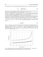
volume fractions. Figure 2.3 presents the typical results of the total transmission and the
total backscattering versus frequency
0
kr
for bubbly gelatin with the parameters 200N = ,
0
1r =
mm, and
3
10
β
−
=
, respectively. The total transmission is defined as
2
||IT= 
, and

Acoustic Waves in Bubbly Soft Media

265
the received point is located at the distance 2rR= from the source. The total backscattering
is defined as
2
|(0)|
N
i
s
i
p

, referring to the signal received at the transmitting source.
It is clearly suggested in Fig. 2.3(a) that there is a region of frequency slightly above the
bubble resonance frequency, i.e., approximately between
0
kr =0.017 and 0.077 in this
particular case, in which the transmission is virtually forbidden. Within this frequencies
range, the Ioffe-Regel criterion is satisfied and a maximal decrease of the diffusion
coefficient
D roughly by a factor of
5
10 is observed and D can thus be considered having
a tendency to vanish, i.e., 0
D → . Here the diffusion coefficient is defined as /3
l
tT
Dvl=
with

t
v being the transport velocity that may be estimated by using an effective medium
method [32]. Indeed, this is the range that suggests the acoustic localization where the
waves are considered trapped [24], confirming the conjectured existence of the phenomenon
of localization in such a class of media. Outside this region, wave propagation remains
extended. For the backscattering situation, the result shows that the backscattering signal
persists for all the frequencies, and an enhancement of backscattering occurs particularly in
the localization region. As has been suggested by Ye et al, however, the backscattering
enhancement that appears as long as there is multiple scattering can not act as a direct
indicator of the phenomenon of localization [28]. In the following we shall thus focus our
attention on the transmission that helps us to identify the localization regions, rather than
the backscattering of the propagating wave.


Fig. 2.3. The total transmission (a) and the total backscattering (b) versus frequency
0
kr for
bubbly gelatin.
Since the sample size is finite, the transmission is not completely diminished in the localization
region, as expected [24]. In this particular case, there exists a narrow dip within the localization
region between
0
kr =0.017 and 0.024, hereafter termed severe localization region, in which the
most severe localization occurs. The waves are moderately localized between
0
kr =0.024 and
0.077, termed moderate localization region, due to fact that the finite size of sample still
enables waves in this region to leak out [15]. We find from Fig. 2.3 that for such systems of
internal resonances, the waves are not localized exactly at the internal resonance, rather at
parameters slightly different from the resonance. This indicates that mere resonance does not

promise localization, supporting the assertion of Rusek et al

[33] and Alvarez et al [34].

Waves in Fluids and Solids

266
To identify the phenomenon of localization by inspecting the correlation characteristics of
the wave field in bubbly soft media, the total correlation functions are numerically studied
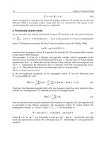
for various frequencies and bubble parameters. Figure 2.4 illustrates the typical result of the
comparison between the total correlation functions for bubbly gelatin at three particular
frequencies chosen as below, within, and above the localization region:
0
kr =0.012, 0.018, and
0.1, referring to Fig. 2.3. Here the parameters of bubbles are identical with those used in Fig.
2.3. Observation of Fig. 2.4 clearly reveals that the total correlation decays rapidly along the
distance
ξ
in the case of
0
kr =0.018, while the decrease of correlation with the increase of
ξ
is very slow in the cases of
0
kr =0.012 and
0
kr =0.1. Such spatial correlation behaviors may
be understood by considering the coherent and the diffusive portions of the transmission.
Here the coherent portion is defined as
2

||
C
IT=  , and the diffusive portion is
DC
III=− .
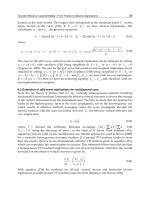
Figure 2.5 plots the total transmission and the coherent portion versus frequency
0
kr for
bubbly gelatin with the parameters used in Fig. 2.4. It is obvious that the coherent portion
dominates the transmission for most frequencies, while the diffusive portion dominates
within the localization region. This is in good agreement with the conclusion drawn by Ye et
al for bubbly liquids (cf. see Fig. 1 in Ref. [24]). As a result, there exist strong correlations
between pairs of field points even for a considerable large distance within the non-localized
region where the wave propagation is predominantly coherent. Contrarily, within the
localization region almost all the waves are trapped inside a spatial domain and the
fluctuation of wave field at a spatial point fails in interacting effectively with any other point
far from it. These results suggest that proper analysis of the spatial correlation behaviors
may serve for a way that helps discern the phenomenon of localization in a unique manner.


Fig. 2.4. The total correlation versus distance
ξ
for bubbly gelatin at three particular
frequencies chosen as below, within, and above the localization region, respectively.

Acoustic Waves in Bubbly Soft Media

267

Fig. 2.5. The total transmission and the coherent portion versus frequency

0
kr for bubbly
gelatin.
3. Phase transition in acoustic localization in bubbly soft media
In this section, we focus on the localization in bubbly soft medium with the effect of
viscosity taken into account, by inspecting the oscillation phases of bubbles rather than the
wave fields. It will be proved that the acoustic localization is in fact due to a collective
oscillation of the bubbles known as a phenomenon of “phase transition”, which helps to
identify phenomenon of localization in the presence of viscosity.
3.1 The influence of viscosity on acoustic localization
So far, we have considered the localization property in a bubbly soft medium, which is
regarded as totally elastic for excluding the effects of absorption that may lead to ambiguity
in data interpretation.
In practical situations, however, the existence of viscosity effect may
notably affect the propagation of acoustic waves and then the localization characteristics in a
bubbly soft medium. Note that the practical sample of a soft medium is in general assumed
viscoelastic [6] and the existence of viscosity inevitably causes ambiguity in differentiating
the localization effect from the acoustic absorption which might result in the spatial decrease
of wave fields as well [36].

In the presence of viscoelasticity, the Lamé coefficients of the soft
medium may be rewritten as below:

ev
t
λλλ
∂
=+
∂
,

ev
t
μμ μ
∂
=+
∂
, (3.1)
where
e
λ
and
e
μ
are the elastic Lamé coefficients,
v
λ
and
v
μ
are viscosity factors given by
Kelvin-Voigt viscoelastic model. In the following we shall assume
v
λ
=0, as is usually done
for a soft medium [35]. The viscosity factor
v
μ
may be manually adjusted in the numerical
simulations to inspect the sensibility of the results to the absorption effects.

Waves in Fluids and Solids

268
Note that the acoustic wave is a simple harmonic wave of angular frequency ω. Then the
longitudinal wave number in the soft viscoelastic medium becomes a complex number as
/
l
kkik c
ω
′′′
=+ =


. Here the real and the imaginary parts represent the propagation and the
attenuation of the longitudinal wave in a soft viscoelastic medium, respectively, and
l
c


refers to the effective speed of the wave. For the acoustic wave that propagates in a soft
viscoelastic medium permeated with bubbles, the influence of the viscosity effect may be
ascribed to two aspects: (1) the propagation of the acoustic wave in a soft viscoelastic
medium should be described by a series of complex parameters instead of the
corresponding real parameters (i.e.,
kk→

,
ll
cc→


, etc.) to account for the absorption
effects; (2) the dynamical behavior of an individual bubble will be greatly affected by the
friction damping of pulsation that results from the viscoelastic solid wall. The incorporation
of the effect of acoustic absorption due to viscosity effects amounts to adding a term
/dU dt
ν
⋅
in the dynamical equation of a single bubble in a soft elastic medium [8].

Here
2
0
4/( )
v
r
νμρ
=
is a coefficient characterizing the effect of acoustic absorption. By seeking the
linear solution of the modified dynamical equation in a same manner as in Section 2.3, one
may derive the scattering function
f
of a single bubble in a soft viscoelastic medium, as
follows:

0
22
00
(/ 1 / /)
l
r

f
ir c i
ωω ω νω
=
−− −
, (3.2)
where
ω
0
refers to the resonance frequency of an individual bubble in a soft medium. On
condition that the soft medium is totally elastic, the expression of the scatter function
f
degenerates to Eq. (2.6) due to the vanishing of the term
/i
ν
ω
− . In such a case, the acoustic
field in any spatial point can thus be solved exactly in a same manner as in Section 2.4.
By rewriting the complex coefficient
i
A
in Eq. (2.10) as
exp( )
ii i
A
Ai
θ
=
with the modulus
and the phase physically represent the strength of secondary source and the oscillation

phase, respectively. For the
ith bubble, it is convenient to assign a two-dimensional unit
phase vector,
ˆ
ˆ
cos sin
ii i
x
y
θθ
=+u
to the oscillation phase of the bubble with
x
ˆ
and y
ˆ

being the unit vectors in the
x and y directions, respectively. The phase of emitting source is
set to be zero. Thereby the oscillation phase of every bubble is mapped to a two-dimensional
plane via the introduction of the phase vectors and may be easily observed in the numerical
simulations by plotting the phase vectors in a phase diagram.
In actual experiments, it is the variability of signal that is often easier to analysis [36].

Hence
the behavior of the phases of the oscillating bubbles may be readily studied by inspecting
the fluctuation of the oscillation phase of bubbles is investigated as well. Here the
fluctuation of the phase of bubbles is defined as follows [36]:

2
22
i
i1
1
δ
N
N
θθθ
=


=−





,
where
i
i1
1
N
N
θθ
=
=

is the averaged phase.

Acoustic Waves in Bubbly Soft Media

269
3.2 Localization and phase transition in bubbly soft media
Figure 3.1 displays the typical results of the phase diagrams for a bubbly gelatin at different
driving frequencies, with the values of viscosity factors manually adjusted to study the
influence of the effect of acoustic absorption. Three particular frequencies are employed (See
Fig. 2.3):

ωr
0
/c
l
=0.01 (Fig. 3.1(a), below the localization region), ωr
0
/c
l
=0.1 (Fig. 3.1(b), above
the localization region), and
ωr
0
/c
l
=0.02 (Figs. 3.1(c) and (d), within the localization region).
In a phase diagram, each circle and the corresponding arrow refer to the three-dimensional
position and the phase vector of an individual bubble, respectively. In Figs. 3.1(a-c) we
choose the viscosity factor as
v
μ

=0, i.e., the soft medium that serves as the host medium is
assumed totally elastic; while in Fig. 3.1(d) the value of viscosity factor is set to be
v
μ
= 50P
(1P=0.1Pa·s). For a comparison we also examine the spatial distribution of the wave fields
and plot the transmissions as a function of the distance from the source in Fig. 3. 2 in cases
corresponding to Fig. 3.1. Note that the energy flow of an acoustic wave is conventionally
2
i
~ p
θ
∇J
. This mathematical relationship reveals the fact that the gradient of oscillation
phases of bubbles is crucial for the occurrence of localization. Apparently, when the
oscillation phases of different bubbles exhibit a coherent behavior (i.e.
i
θ
is a constant) while
p
is nonzero, the acoustic energy flow will stop and the acoustic wave will thereby be
localized within a spatial domain [36]. Moreover, such coherence in oscillation phases of
bubbles is a unique feature of the phenomenon of localization that results from the multiple
scattering of waves, but lacks when other mechanism such as absorption effect dominates,
as will be discussed later. Consequently, it should be promising to effectively identify the
localization phenomenon by giving analysis to the oscillation phases of bubbles and seeking
their ordering behaviors.
It is apparent in Figs. 3.1(a) and (b) that the phase vectors pertinent to different bubbles
point to various directions as the driving frequency of the source lies outside the localization
region. In other words, the oscillation phases of the bubbles located at different positions in

a bubbly soft medium are random in non-localized states. Correspondingly, the curves 1
(thin solid line) and 2 (thin dashed line) in Fig. 3.2 shows that the non-localized waves
remain extended and can propagate through the bubble cloud. As observed in Fig. 3.1(c),
however, the phase vectors located at different spatial positions point to the same direction
when localization occurs, which indicates that the oscillation phases of all bubbles remain
constant and the energy flow of the wave stops.

The transition from the non-localized state
to the localized state of the wave can be interpreted as a kind of “phase transition”, which is
characterized by the unusual phenomenon that all the bubbles pulsate collectively to
efficiently prohibit the acoustic wave from propagating [10]. Such a concept of phase
transition is physically consistent with the order-disorder phase transition in a ferromagnet
[37]. Note that the phase of emitting source is assumed to be zero in the numerical
simulations, i.e., the phase vector at the source points to positive
x
ˆ
direction, while all the
phase vectors in Fig. 3.1(c) point to the negative
x
ˆ
-axis. This means that as the localization
occurs, almost all bubbles tend to oscillate completely in phase but exactly out of phase with
the source, which leads to the fact that the localized acoustic energies are trapped within a
small spatial domain adjacent to the source as shown by the curve 3 (thick solid line) in Fig.
3.2. These numerical results are consistent with the previous conclusions obtained for
bubbly water and bubbly soft elastic media [10,36]. Therefore it is reasonable to conclude
that such a phenomenon of phase transition is the intrinsic physical mechanism from which
the acoustic localization stems.

Waves in Fluids and Solids

270

Fig. 3.1. The phase diagrams for the oscillating bubbles in a bubbly gelatin with different
structural parameters: (a)
ωr
0
/c
l
=0.01, μ
v
=0; (b) ωr
0
/c
l
=0.1, μ
v
=0; (c) ωr
0
/c
l
=0.02, μ
v
=0; (d)
ωr
0
/c
l
=0.02, μ
v

=50P.


Fig. 3.2. Transmissions versus the distance from the source in a bubbly gelatin with different
structural parameters.
Note that the effect of acoustic absorption has been completely excluded in Figs. 3.1(a-c)
which may cause ambiguity in identifying the phenomenon of localization. It is thus of
much more practical significance to investigate the localization properties in the case where
soft medium is assumed viscoelastic, and the corresponding results are shown in the phase
diagram given by Fig. 3.1 (d) as well as the comparison between transmissions versus
r in
Fig. 3.2. As the viscosity factors of the soft medium are manually increased, the phenomena
of phase transition can be identified in a bubbly soft viscoelastic medium provided that the

Acoustic Waves in Bubbly Soft Media

271
driving frequency of acoustic wave falls within the localization region. Meanwhile,
exponential decay of the wave fields with respect to the distance from the source is shown
by the curve 4 (thick dashed line) in Fig. 3.2. Observation of Fig. 3.1(d) and Fig. 3.2
apparently manifests that, however, the adjustment of the values of the viscosity factors
leads to changes of the direction to which all the phase vectors point collectively varies and
the decay rates of the transmissions versus
r.
For a bubbly soft viscoelastic medium, it is still possible to achieve the acoustic localization
since the condition can be satisfied that the oscillation phases of bubbles at any spatial
points remain constant, but the extents of localization are necessarily affected by the
presence of viscosity effect. It is thus difficult to differentiate the phenomenon of acoustic
localization from that of the acoustic absorption without referring to the analysis of the
behavior of the phases of bubbles [11]. Notice that in Fig. 3.1, as the viscosity factors are

gradually enhanced, the angles between the directions of the phase vectors and the negative
x-axis increase. This means that the phase-opposition states between the oscillations of all
the bubbles and the source as well as the extents to which the acoustic wave is localized are
weaken due to the enhancement of the viscosity. Therefore it may be inferred that the
occurrence of phase transition in a bubble soft medium is a criterion for identifying the
phenomenon of localization, while the localization extents can be predicted by accurately
analyzing the relationship between the oscillation phases of the bubbles and the source.
It is convenient to employ a phase diagram method for observing the collective phase
properties of the bubbles and thereby seeking the existence of the phenomenon of phase
transition, however the values of the oscillation phase of each bubble could not be directly
read via the phase diagrams in a precise manner. We then illustrate the statistical properties
of the parameters of
θ
for all the bubbles in Fig. 3.3 for a more explicit observation of the
values of oscillation phases of the bubbles. Here
⋅
denotes the ensemble average over
random configurations of bubble clouds,
()p
θ
θ
is defined as the probability that the values
of
θ
fall between
θ
and
θθ
+Δ , i.e.,
θθθ θ

≤<+Δ, with
θ
Δ referring to the difference
between the two neighbor discrete values of
θ
. And the values of ()p
θ
θ
have been
normalized such that the total probability equals 1. In Fig. 3.3 three particular values of
viscosity factors are considered:
v
μ
= 0 (curve 3, thick solid line), 50P (curve 4, thick dashed
line), 200P (curve 5, thick dotted line). It is obvious in Fig. 3.3 that: (1) Outside the
localization region, as shown by the thin curves 1 (solid line) and 2 (dashed line), the values
of oscillation phases
θ
exhibit large extents of randomnesses, which indicates a lack of the
above-mentioned collective behavior of the bubble oscillation crucial for the existence of
localization, in accordance with the results shown in Figs. 3.1(a) and (b). (2) When the
phenomenon of localization occurs, the oscillation phases almost remain constant for
bubbles located at different spatial points, which is illustrated by the delta-function shapes
of the thick curves 3-5. It is also noteworthy that the oscillation phase of each bubble
approximates -
π
in an elastic medium, and that the presence of the viscosity effect does not
change such a phenomenon of phase transition but leads to a larger average value of
oscillation phases
θ

. A monotonic increase of the values of the oscillation phases of
bubbles is clearly observed as the viscosity factors are gradually enhanced. In the soft
medium with viscosity factor
v
μ
=50P, the values of
θ
nearly equal -0.45
π
for all the
bubbles, and
θ
approximate -0.15
π
for the case of
v
μ
=200P.

Waves in Fluids and Solids

272

Fig. 3.3. The comparison between the statistical behaviors of the oscillation phases of
bubbles in a bubbly gelatin with different structural parameters.
The principal influence of the viscosity effect on the localization property in a bubbly soft
medium attributes intrinsically to two aspects of physical mechanism. The localization
phenomenon in inhomogeneities had been extensively proved to stem from the important
multiple scattering processes between scatterers. In a viscoelastic medium the recursive
process of multiple scattering could not be well established due to the effect of acoustic

absorption caused by the viscosity, which necessarily impairs the extent to which the
acoustic wave can be localized. For an individual bubble pulsating in a viscoelastic medium,
on the other hand, the oscillation will be hindered by the friction damping caused by the
viscoelastic solid wall. While the bubble in an elastic soft medium can behave like a high
quality factor oscillator [2], the increase of viscosity factors will definitely reduce the quality
factor that is defined as
Q=ω/υ and then the strength of the resonance response of bubble to
the incident wave. This prevents the bubbles from becoming effective acoustic scatterers,
which is crucial for the localization to take place [24]. As a result, it is perceivable that the
increase of the viscosity effects diminishes the extent to which all bubbles pulsate out of
phase with the source, and a complete prohibition of acoustic wave could not be attained.
Figure 3.4 displays the fluctuations of the oscillation phases of bubbles δ
θ as a function of
the normalized frequency
ωr
0
/c
l
in a bubbly gelatin for four particular values of viscosity
factors:
v
μ
=0, 5P, 50P and 500P. Note also that the fluctuations of the phases approaches
zero at the zero frequency limit due to the negligibility of the scattering effect of bubbles.
The phenomena of phase transitions can be clearly observed characterized by significant
reductions of the fluctuations within particular ranges of frequencies whose locations are in
good agreement with the corresponding frequency regions where the localization occurs.
This is consistent with the previous results obtained for bubbly water. Moreover, it is
apparently seen that the amounts to which the fluctuations δ
θ decrease can act as reflections

of the extents of the acoustic localizations. In a bubbly viscoelastic soft medium, such a
phenomenon of phase transition persists within the localization region, while the increase of
the value of viscosity factor leads to a weaker reduction of the fluctuation of phases. In the
particular case where the viscosity effects are extremely strong, i.e.,

v
μ
=500P, the
localization is absent due to the fact that the effects of multiple scattering and the bubble
resonance are severely destroyed, and the phenomenon of phase transition could not be

Acoustic Waves in Bubbly Soft Media

273
identified. The comparison of Figs. 3.1-3.4 proved that the phenomenon of phase transition
is a valid criterion of the existence of acoustic localization in such a medium, and the values
of the oscillation phases of the bubbles help to determine the extent to which the acoustic
waves are localized. Consequently it is fair to conclude that the proper analysis of the
oscillation phases of bubbles can indeed act as an efficient approach to identify the
phenomenon of acoustic localization in the practical samples of bubbly soft media for which
the viscosity effects are generally nontrivial. The important phenomenon of phase transition
is an effective criterion to determine the existence of localization, while the extent to which
the acoustic wave is localized may be estimated by inspecting the values of the oscillation
phases or the reduction amount of the phase fluctuation.


Fig. 3.4. The comparison between the fluctuations of the oscillation phases of bubbles versus
frequency in a bubbly gelatin with different values of viscosity factors.
4. Effective medium method for sound propagation in bubbly soft media
In this section, we discuss the nonlinear acoustic property of soft media containing air

bubbles and develop an EMM
to describe the strong acoustic nonlinearity of such media
with the effects of weak compressibility, viscosity, surrounding pressure, surface tension,
and encapsulating shells incorporated. The advantages as well as limitations of the EMM are
also briefly discussed.
4.1 Bubble dynamics
Consider an encapsulated gas bubble surrounded by a soft viscoelastic medium. When in
equilibrium, the gas pressure in the bubble is denoted
g
P , and the pressure infinitely far
away is
P
∞
. For the case where the equilibrium pressure equals the surrounding pressure
(i.e.
g
PP
∞
= ), the shear stress is uniform throughout the soft medium. Such a case is referred
to as an initially unstressed state, for which the equilibrium values of the inner and outer
radius of the bubble are designated
0
R and
0s
R , respectively. In the general case, however,
the encapsulated bubble may be pressurized, such that
g
PP
∞
≠ . Such a case is denoted as a

prestressed case due to the fact that a nonuniform shear stress is generated inside the
medium to balance the pressure difference. For a prestressed cases we define the

Waves in Fluids and Solids

274
equilibrium values of the inner and outer radius as
1
R and
1s
R , respectively. The geometry
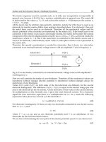
is shown in Fig. 4.1. Figure 4.1(a) shows an unstressed case where one has
0
R =
1
R and
0s
R =
1s
R . In the cases where
g
P < P
∞
, however, it is apparently that the pressure difference
between
g
P and P
∞
will force the bubble to shrink, and one thus has
0

R >
1
R and
0s
R >
1s
R ,
as illustrated in Fig. 4.1(b). In contrast, one has
0
R <
1
R and
0s
R <
1s
R if
g
PP
∞
> . As the
bubble oscillates, the instantaneous values of the inner and outer radius are defined as
()Rt
and
()
s
Rt, respectively.


Fig. 4.1. Geometry of an encapsulated gas bubble in a soft medium in (a) an initially
unstressed state and (b) a prestressed state.

Zabolotskaya et al [6] has studied the nonlinear dynamics in the form of a Rayleigh-Plesset-
like equation for an individual bubble in such a model, and provided the approaches to
include the effects of compressibility, surface tension, viscosity, and an encapsulating shell.
Note that Eq. (53) in Ref. [6] accounts for the effects of surface tension, viscosity, and shell
but applies only to the case of an incompressible medium. Adding the compressibility term
33
(/)/
m
dw dt c that accounts for the radiation damping to the left hand side of this equation,
one readily obtain the equation that describes the nonlinear oscillation of a single bubble in
a soft medium, as follows:

23
23
1
23
33
33
311
() ()
2
2
24
() 1 ,
g
mm
g
m
esm
sss

dR dR dw R
FRR GR P P
dt dt c dt R
dR R R
PR
RRRdt R R
γ
ρ
σ
σ
ηη
∞


 
+−= −

 
 







−−−− −+


 








(4.1)
In the preceding expression, the parameter w is defined as
3
/3wR= ,
2/ 2/
g
ms
PRR
σ
σσ
=+ is the effective pressure due to the surface tension with
g
σ
and
m
σ

being the surface tensions at the inner gas-shell interface and the outer shell-medium
interface, respectively, and
ψ
is the dissipation function that is found to be
23333
8(/) (1 /) /

ssms
RdR dt R R R R
ψπ η η


=−+


with
s
η
and
m
η
being the shear viscosity
coefficients in the shell region and in the medium, respectively, the parameters of
()FR and
()GR are given as

Acoustic Waves in Bubbly Soft Media

275
() 1 ,
ss
mms
R
FR
R
ρρ
ρρ


=+−



3
3
41
() 1
33
ss
mm ss
RR
GR
RR
ρρ
ρρ
 
=+− −
 
 

with
s
ρ
and
m
ρ
are the mass densities of the shell and the surrounding medium,
respectively, and

()
e
PR refers to the effective pressure due to the strain energy stored in
shear deformation of both the shell and the medium, defined as [6]

224 2 24
224 2 24
12 1 2
() 4 4 ,
s
s
R
ss mm
e
rR
rrrdr r rrdr
PR
IrI rrr I rI rrr
εε ε ε
∞
  
 
∂∂ ∂ ∂
=+ −++ −
  
 
∂∂ ∂ ∂
 
  



  
(4.2)
where
123
(,,)III
εε
= refers to the strain energy density with
1
I ,
2
I ,
3
I being the principal
invariants of Green’s deformation tensor,
r
and r

refer to the Eulerian and the Lagrangian
coordinates, respectively, the subscripts s and m refer to the shell and for the surrounding
medium, respectively.
For the convenience of the following investigation, we will evaluate Eq. (4.1) here in the
quadratic approximation by rewriting it into another form for the perturbation in bubble
volume defined as
33
1
4( )/3URR
π
=− . For a soft medium Mooney’s constitutive relation
[38]

is the most widely used model equation and has been adopted by many previous
studies regarding the nonlinear dynamics of a bubble in such a medium [3-6].

For facilitating
the comparison with the previous studies, therefore, we employ Mooney’s relation to
evaluate the effective pressure
()
e
PR, as follows:

[
]
12
(1 )( 3) (1 )( 3) 4, ,
pp
II psm
εμ χ χ
=+−+−− = (4.3)
where
p
μ
is the shear modulus.
Substituting Eq. (4.3) into Eq. (4.2) and expanding
()
e
PR to quadratic order, one may derive
an analytical approximation of
()
e

PR, as follows:
2
11111
() () ()( )()( ) ()/2
eee e e
PR P P P P
ζζζζζζζζ
′′
′
== +− +− ,
where
0
/RR
ζ
= ,
110
/RR
ζ
= , the primes represent derivatives with respect to
ζ
, and the
parameters of
()
e
P
ζ
, ( )
e
P
ζ

′
, and ( )
e
P
ζ
′′
are given as below:

178 156
0
1
178 156
() (1 )( ) (1 )( )
(1 )( ) (1 )( ) ,
a
em
s
a
Pyxyxyyxdx
y
xyx yyxdx
ζμ χ χ
μχ χ
−− −−
−− −−

=+−+−−


++ −+−−




(4.4a)

210842286
0
1
2 108 42 2 86
( ) (1 )(7 ) (1 )( 5 )
(1 )(7 ) (1 )( 5 ) ,
a
es
m
a
Pyxyxyyxdx
y
x
y
x
yy
xdx
ζμζ χ χ
μζ χ χ
−− −
−− −
′

=+ −+−+



++ −+−+



(4.4b)

4721385116
0
1
4721385116
( ) (1 )(4 70 ) (1 )(2 40 )
(1 )(4 70 ) (1 )(2 40 )
2()/,
a
es
m
a
e
Pyxyxyyxdx
y
x
y
x
yy
xdx
P
ζμζ χ χ
μζ χ χ
ζζ

−− −
−− −
′′

=+−−−+



++−−−+


′
+


(4.4c)

Waves in Fluids and Solids

276
where
0
/xR r=

,
0
/
y
Rr= ,
00

/
s
aR R= .
Substituting Eq. (4.4) into Eq. (4.1), one obtains the expansion of Eq. (4.1) to quadratic order
in U , as follows:

23
22
1
11 12
23
1
2
2
11
2
2,
m
A
dU dU R dU dU
UGUU
dt dt F c dt dt
dU d U
HUeP
dt dt
δω δ
++− =+


++−






(4.5)
where
0
()
A
Pt P P
∞
=− is the applied acoustic pressure with
0
P being the pressure at infinity
in the absence of sound,
222
1 ge
σ
ωωωω
=+− is the nature frequency of bubble for which the
components are given as
2
1
3
gg
PD
ωγ
= ,
2

111
()
ee
PD
ωζζ
′
=
,
21 4
11
2( )
g
mR
DR
σ
ωσσ
γ
−
=+,
γ
is the ratio of specific heats which is chosen as
γ
=1.4 since the we only consider air
bubbles in the present study,
1
δ
and
2
δ
are the viscous damping coefficients at linear and

quadratic order, respectively, defined as
()
33
11
41
sRmR
D
δη
γ
η
γ


=−+


,
()
66
211
24 1
sRmR
qD
δη
γ
η
γ


=−+



,
1
G is the nonlinearity coefficient associated with gas compressibility, elasticity, and surface
tension that is defined as
()
2223
11 1
11
4
11
1
() 8
3( 1) 2 4 1
()
em
ge R
ms
e
PR
Gq
FR
P
σ
ζζ σ
γω ωω γ
ρ
ζ




′′



=++− −+ −

′





,
and the parameters of
1
F ,
1
H ,
1
e ,
1
q ,
ρ
γ
,
R
γ
and

1
D are given as follows

1
(1 )
R
F
ρρ
γγγ
=+− ,
14
111
(1 )HqF
ρρρ
γγγ
−


=+−


,
3
111
4eDR
π
= ,
3
11
1/(8 )

q
R
π
= , /
sm
ρ
γρρ
= ,
11
/
Rs
RR
γ
= ,
2
111
1/( )
m
DFR
ρ
= .
4.2 Effective medium method
4.2.1 Effective medium
We now study the propagation of a plane acoustic wave in an infinite soft medium
containing random encapsulated bubbles, subject to the condition that the volume content
of the bubbles is small but the number of bubbles on a scale of wavelength order is large.
Then it can be proved that the multiple scattering effects are negligible [39] and the
homogeneous approximation well known for liquid containing bubbles can be employed
[3]. Consider a small volume element of the medium of length
i

dx in the
i
x direction in the
Cartesian coordinate (i=1, 2, 3) that is sufficiently large to include a number of bubbles. In
the present study, we shall focus our attention on the cases where the amplitude of wave is
small, for the purpose of investigating the strong physical nonlinearity of such a class of
media [3,4]. Then the dynamic nonlinearity is negligible that dominates only on condition
that the amplitude of wave is finite. According to the stress-strain relationship and

Acoustic Waves in Bubbly Soft Media

277
neglecting the contribution of the gas inside the bubbles, the stress tensor may be expressed
as (see Ref. [7], pp. 10)
(1 ) 2 ( /3)
ll ll
ssss
ik ik ik ik
Ku u u
σβδμδ


=− + −


, (4.6)
where
s
ik
σ

and
ik
s
u are the stress tensor and the strain tensor of the solid phase,
β
is the total
volume fraction of the bubbles, 2 /3K
λ
μ
=+ is the bulk modulus,
ik
δ
refers to the
Kronecker delta which is defined as
1,
0,
ik
ik
ik
δ
=

=

≠

.
On the other hand, the volume element of the bubbly soft medium may be regarded as a
volume element of “effective” medium that is homogeneous and is described by effective
acoustical parameters. The stress tensor of the effective medium may be given as below:

2( /3)
ik ll ik ik ik ll
Ku u u
σδμδ
=+−



, (4.7)
where
ik
σ

and
ik
u

are the stress tensor and the strain tensor of the effective medium,
respectively, 2 /3K
λμ
=+


is the effective bulk modulus with
λ

and
μ

being the effective

Lamé coefficients of the effective medium.
4.2.2 Influence of bubble oscillation
As the acoustic wave propagates in the bubbly medium, the volume of the bubbles will
change due to the oscillation of the bubbles driven by the acoustic wave. As a result, the
variation of the volume element includes the compression of the elastic phase and the
variation of the total volume of the bubbles. Then one has
(1 )
s
t
V
θθ β
=−+

, (4.8)
where
11 22 33
uuu
θ
=++


and
11 22 33
ss s s
uuu
θ
=++ are the volume changes of the effective
medium and the elastic phase, respectively,
t
V is the variation of the specific volume of

bubbles.
As the bubble distorts under the action of the shear deformation, the principal radii of
curvature of the surface will change. This will certainly change the effect of surface tension
and then the bubble volume. In the present study, however, the bubbles are assumed
spherical, and such an effect is then negligible that does not change the nature of the bubble
dynamics. Then it is fair to assume approximately that the pure shear deformation of the
volume element will not affected by the existence of bubbles. Then one has
,.
ss
ik ik ik ik
uu ik
σσ
==≠


(4.9)
Substituting Eq. (4.9) into Eqs. (4.6) and (4.7) yields
(1 )
μμ β
=−

.
From Eqs. (4.6) and (4.7) one readily obtains

11 22 33
3(1 )( 2 / 3)
sss s
σσσ
β
λ

μ
θ
++=− + , (4.10a)

Waves in Fluids and Solids

278

11 22 33
3( 2 / 3)
σσσ λμθ
++=+

 
(4.10b)
Under the action of an applied force, the element of effective medium is defined to produce
the same stress as the element of the bubbly medium. Hence one has

11 22 33 11 22 33
sss
σσσσσσ
++=++

(4.11)
Substituting Eqs. (4.8-4.10) into Eqs. (4.6) and (4.7) yields (for
λμ
>> )

11 11
()

ss
t
CC V
θθ
=−

(4.12)
where
11
2C
λ
μ
=+
,
11
2C
λ
μ
=+



are the elastic modulus of the soft medium and the
effective medium, respectively.
For the purpose of solving the unknown quantity
t
V
, it is necessary to obtain the variation
of the volume of an individual bubble U which is described by the equation for the
oscillation of a bubble given by Eq. (4.5). In Eq. (4.5), the acoustic pressure

A
P
accounts for
the driving force of the oscillation of the bubble. Due to the fact the shear wave does not
change the volume of the bubble, the driving force of the bubble oscillation is not affected by
the shear wave but determined by the total radial force exerted by the incident wave [3].
According to Eq. (17) in Ref. [3] one has

2/3
2
A
P
λμ
σσ
λμ
+
=
+

, (4.13)
where
11
σσ
=

is the pressure generated by the incident wave.
Substituting Eq. (4.13) into Eq. (4.5) yields

23
22

1
11 12
23
1
2
2
11
2
2,
m
dU dU R dU dU
UGUU
dt dt F c dt dt
dU d U
HUe
dt dt
δω δ
σ
++− =+


++−





(4.14)
Owing to the fact that Eq. (4.14) is nonlinear only to second order, a potential solution has
the form

12
exp( ) exp( 2 ) . .UU it U i t cc
ωω
≈+ +, (4.15a)

12
()exp( ) ()exp(2 ) it i t cc
σσ ω σ ω
≈+ +rr , (4.15b)
where
1
σ
and
2
σ
refer to the linear and the nonlinear waves, respectively,
1
U and
2
U refer
to the amplitude of the linear pulsation and the nonlinear response, respectively,
r refers to
the three-dimensional space coordinate position of the field point that may be expressed in
the Cartesian coordinate as
12 3
ˆ
ˆˆ
xi x
j

xk=++r .
Substituting Eq. (4.15) into Eq. (14) and assuming that
12
1 UU>> yield

111
Ug
σ
= ,
2
222 1
Ug
σσ
=+Γ, (4.16)

Acoustic Waves in Bubbly Soft Media

279
where
1
1
22 3
111
()( /)
m
e
g
iRc
ωω ωδω
=−

−+ +
,
1
2
22 3
111
(4)(2 8 /)
m
e
g
iRc
ω ω ωδ ω
=−
−+ +
,
2
2
112
1
22 3
111
(3 )
(4)(2 8 /)
m
GHi
g
iRc
ωωδ
ωω ωδω
−+

Γ=
−+ +
,
Expanding the displacement vector
u , up to second order approximation, as
12
()exp( ) ()exp(2 ) it i t cc
ωω
=+ +uur ur ,
one obtains

(1)
111 1
C
σ
=∇⋅u

,
(2)
211 2
C
σ
=∇⋅u

(4.17)
If the size distribution function of the bubbles is specified as
0
()nR
(so that
00

()nR dR
is the
number of bubbles with radii from
0
R
to
00
RdR+
in unit volume), the variation of the
specific volume of the bubbles
t
V
is related to the volume variation of an individual bubble
U by the relationship

00
()
t
VUnRdR=

, (4.18)
Expanding
t
V to second order approximation as

12
exp( ) exp( 2 ) . .
t
VV itV itcc
ωω

=+ +, (4.19)
one obtains from Eqs. (4.16-4.19)

(1)
1111 1
g
VVC=∇⋅u

,
()
2
(2) (1)
2211 2 111
g
VVC VC
Γ
=∇⋅+∇⋅uu

(4.20)
where
1100
()
g
V
g
nR dR=

,
2200
()

g
V
g
nR dR=

, and
00
()VnRdR
Γ
=Γ

.
If all the bubbles are of the uniform radius
0
R ,
t
V is related to U by the relationship
t
VNU= with
31
0
3(4 )NR
βπ
−
= being the number of bubbles in unit volume. In such cases
one has
11g
VN
g
= ,

22g
VN
g
= , VN
Γ
=Γ.
Expressing the volume change of the solid phase as
s
θ
=∇⋅u , one may rewrite Eq. (4.12) as
follows:

(1)
11 1 11 1 1
()CCV∇⋅ = ∇⋅ −uu

,
(2)
11 2 11 2 2
()CCV∇⋅ = ∇⋅ −uu

. (4.21)
4.2.3 The wave equations
According to Ref. [6],
1m
F
ρ
is defined as the effective density of the soft medium
surrounding the bubbles, the effective density of the effective medium may thus be

Waves in Fluids and Solids

280
identified as
1
(1 )
mg
F
ρρ β ρβ
=−+

. Since the dynamic nonlinearity of the medium
associated with the finite amplitude of wave has been ignored, the wave equation of the
effective medium may be written as follows:

2
11
2
()C
t
μρ
∂
∇ ∇⋅ − ∇×∇× =
∂
u
uu



, (4.22)

We represent the displacement vector
u in terms of the sum of the potentials, as follows:

=∇Φ+∇×u Ψ , (4.23)
for which the vector potential
Ψ satisfies 0∇⋅ =Ψ .
Up to second order approximation, the scalar potential
Φ may be written as

(1) (2)
ccΦ≈Φ +Φ + , (4.24)
where

(1)
1
(,) ()exp( )tit
ω
Φ =Φrr ,
(2)
1
(,) ()exp(2 )tit
ω
Φ =Φrr . (4.25)
Substitution of Eqs. (4.23) and (4.24) in Eq. (4.22) yields

(1)
2
(1) (1)
2
11

2
C
t
ρ
∂Φ
∇Φ =
∂


,
(2)
2
(2) (2)
2
11
2
C
t
ρ
∂Φ
∇Φ =
∂


, (4.26)

2
2
2
t

μρ
∂
∇=
∂
Ψ
Ψ


. (4.27)
As observed from Eq. (4.27), this equation takes on a non-resonant form and the influence of
the existence of the bubbles on the propagation of the shear wave in a bubbly soft medium is
insignificant. In the following we shall restrain our attention in the propagation of the
compressional wave in such a medium.
Substituting Eqs. (4.20), (4.21), and (4.25) in Eq. (4.26), we arrive at the equations that must
be satisfied by the scalar potentials of the first and the second order, as follows:

22
11 1 1 11 1
(1 ) 0
g
CVC
ρω
∇Φ + + Φ =

, (4.28a)

()
()
2
2

(1)
22 2
11 2 2 11 2 11 11 1
4(1 )
g
CVCCVC
ρω
Γ
∇Φ + + Φ = ∇Φ


, (4.28b)
Eqs. (4.28a) and (4.28b) give description of the the propagation of the fundamental and the
second harmonics of the compressional wave in a bubbly soft medium, respectively. Note that
Eq. (4.28) is derived on the basis of Eq. (4.22) which is expressed as a form of a linear order
terms with nonlinear propagation parameters due to the nonlinear oscillation of bubbles.
Consequently it is seen that Eq. (4.28b) takes a simple form without any quadratic term
involved that represents the dynamic nonlinearity caused by the finite amplitude of wave. In
the right hand side of this equation, however, a quadratic term appears that accounts for the
transfer of acoustical energy from the fundamental to the second harmonic waves, which
results from the strong physical nonlinearity that dominates for a bubbly medium.

Acoustic Waves in Bubbly Soft Media

281
4.2.4 One-dimensional case
Now consider a one-dimensional case in which a plane longitudinal wave propagates along
the
1
ˆ

x
direction in a bubbly soft medium. For simplicity while without losing generality, we
assume that all the bubbles are of the same equilibrium radius
0
R . In such a case Eq. (4.25)
becomes

(1)
111
(,) ()exp( )xt x it
ω
Φ =Φ ,
(2)
121
(,) ()exp(2)xt x i t
ω
Φ =Φ . (4.29)
Using the Kelvin-Voigt viscoelastic model, the Lamé coefficients of the soft viscoelastic
medium may be rewritten as

m
λλ
= , /
mm
t
μμ η
=+∂∂. (4.30)
Substitution of Eqs. (4.29) and (4.30) in Eq. (4.28) yields

2

22
1
111
2
1
()0
g
d
V
dx
ρω
Φ
+Λ+ Φ=

, (4.31a)

2
22 242
2
222 1
2
1
(4 )
g
d
VV
dx
ρω ρ ω
Γ
Φ

+Λ+ Φ= Φ

, (4.31b)
where
[
]
22
1
(2)2
mm m
i
ω
ρ
λμ ωη
Λ= + +

, and
[
]
22
2
4(2)4
mm m
i
ω
ρ
λμ ωη
Λ= + +

.

We introduce the effective wave numbers defined as complex numbers that can be
expressed in terms of real effective wave speeds and effective attenuations, as follows:
22
11 1 11
/
g
kVci
ρ
ωωα
=Λ+ = −


,
22
22 2 22
42/
g
kVci
ρ
ωωα
=Λ+ = −


,
where
i
k

refers to the effective wave numbers,
i

c and
i
α
refer to the (real) effective wave
speed and the effective attenuation, respectively; and the subscripts
i =1, 2 refer to the
fundamental wave and the second harmonic wave, respectively.
Assuming
11 11
exp( )
A
ik xΦ =Φ −

, from Eq. (4.31a) one readily obtains the expressions of
1
c
and
1
α
, as follows:

12
22
111
1
2
AAB
c
−


−+ +

=


,
111
2Bc
αω
= . (4.32)
where the parameters of
2
A
,
2
B
, and C are given as follows:
22
2
11
1
222222 3 2
111
2()
(2)4 ( )( /)
mm
mm m m
Ne
A
Rc

λμ ωω
ρω
λμ ωηωω ωδω


+−
=−


++ −++



,
3
2
11 1
1
222222 3 2
111
2(/)
(2)4 ( )( /)
mm
mm m m
Ne R c
B
Rc
ωη ωδ ω
ρω
λμ ωηωω ωδω



+
=−


++ −++



.
It is apparent that the solution of Eq. (4.31b) is supposed to consist of a general solution and
a special solution. By invoking the boundary condition that the second harmonic wave

Waves in Fluids and Solids

282
should be zero at the beginning, i.e.,
1
20
0
x =
Φ=, one can readily determine the expression of
the second harmonic wave as follows:

2
21 2 2
exp( ) exp( ) . .
gA
Cikxikxcc


Φ=Φ −−− +


, (4.33)
where

12
22
222
2
2
AAB
c
−

−+ +

=


,
222
Bc
αω
= . (4.34)
where the parameters of
2
A ,
2

B and C are given as follows:
22
2
11
2
222222 3 2
111
2(4)
(2)16 (4)(2 8 /)
mm
mm m m
Ne
A
Rc
λμ ωω
ρω
λμ ωηωω ωδω


+−
=−


++ −++



,
3
2

11 1
2
2 22222 3 2
111
4(28/)
(2)16 (4)(2 8 /)
mm
mm m m
Ne R c
B
Rc
ωη ωδ ω
ρω
λμ ωηωω ωδω


+
=−


++ −++



.
[
]
22
11 22 21 12 1 2
()()()CMNMNiMNMN NN=++− +

,
where
24 2 2 2 2
111111112
(3 )( )2MNeGHABAB
ρ
ωω ωδ


=−−+



,
24 2 2 2 2
211121111
()2(3)MNeAB ABGH
ρω ωδ ω


=−−−



,
11 12 12 1
(4 ) ( 4 )NK AA LB B=− + + − ,
21 1 2 12 1
(4 ) ( 4 )NL AA KB B=− + − − ,
where

22222 3 2
11 1 1 1
22 3 3
111 11
(4)( )( /)
2( )( / )(2 8 / ),
m
mm
KRc
Rc Rc
ωωωω ωδω
ωωωδω ωδ ω

=− − − +

−− + +

222 3 2 3
11 1 1 1 1
2222 3
1111
()( /)(28/)
2( 4 )( )( / ).
mm
m
LRcRc
Rc
ωω ωδω ωδ ω
ωωωωωδω


=−−+ +

+− − +

In practical, the nonlinearity parameter
(/)BA is of particular significance that may be
used to define the nonlinearity of the media. In the present study, therefore, we introduce
an effective nonlinearity parameter
(/)
e
BA to describe the extent to which the
nonlinearity of a bubbly medium is enhanced by the nonlinear oscillation of bubbles. The
value of
(/)
e
BA may be determined near the natural frequency of bubble, as given
below:

[39]

Acoustic Waves in Bubbly Soft Media

283
3
12
4(2 )
(/) 2
mm
e
Cc

BA
ραα
ω
−
=−

It is apparent that the expression of the effective nonlinearity parameter
(/)
e
BA derived
here is identical in form with the one obtained by Ma et al except that their approach only
applies to a liquid containing shelled bubbles [39].
Despite the similarity between the EMM and other methodologies which also investigate the
wave propagation in inhomogeneities by treating the media as a homogeneous effective
medium [40-45], the EMM definitely differs from them in several respects. It is a
fundamental distinction that the EMM accounts for the nonlinearity of the bubbly soft
medium up to a second-order approximation, whereas most of the previous ones only use
linear approximation when homogenizing the medium [40-43], which inevitably loses
significant details for bubbly soft media with particularly strong “physical” nonlinearity
[3,4]. Second, the EMM permits one to take into consideration the effects of weak
compressibility, surface tension, viscosity, surrounding pressure, and an encapsulating
elastic shell, which can only be partially accounted for by other methods [44,45]. There are
important practical reasons for pursuing more precise results in various engineering
situations, for which the incorporation of these effects is apparently necessary. (For a
detailed discussion on this topic and a comparison between the application of the EMM and
some other methods in different cases serving as simple models of practical situations, see
Ref. [12]) Finally, the EMM could apply to three-dimensional cases rather than one-
dimensional cases. Most of the relative studies investigate only the wave propagation in an
infinite effective medium for which the one-dimensional approximation is sufficient, but it is
indispensable to obtain the three-dimensional effective parameters for some practical

structures of finite sizes.
It must be stressed, however, that there also exist limitations of the application of the EMM
despite its effectiveness. First, the multiple scattering effects have been neglected when we
homogenizing the bubbly soft medium, therefore the EMM can not apply to bubbly media
with extremely large volume fractions. Second, the EMM is developed under quadratic
approximation by employing a simple perturbation approach, and the nonlinearity of
medium is studied by inspecting the second harmonic wave with no harmonics of orders
higher than 2 involved. Finally, the present model could not enable full incorporation of all
the practical effects that affect the acoustical properties of a bubbly medium, such as the
buckling of bubbles [46]. These problems will be the focus of a future study.
5. Optimal acoustic attenuation of bubbly soft media
In this section, we present an optimization method on the basis of fuzzy logic (FL) and genetic
algorithm (GA) to obtain the optimal acoustic attenuation of a longitudinal wave in a bubbly
soft medium by optimizing the parameters of size distribution of bubbles. This optimization
method can be used to design acoustic absorbent with uniformly high acoustic attenuation
within the frequency band of interest, without the precise mathematical model required.
5.1 Acoustic attenuation in bubbly soft media
The oscillation of an air bubble in a soft medium is special, due to the fact that only if the
ratio λ/μ is sufficiently large can this bubble behave effectively as a resonant oscillator [7].
When compared with the viscoelasticity of the medium, the resonance of the system

Waves in Fluids and Solids

284
introduced by bubbles becomes the most dominant mechanism for acoustic attenuation [13].

For a bubbly soft medium, it is apparent that the acoustic properties are affected by all the
structural parameters, of the bubbles and of the medium. By employing the EMM presented
in Section 4, we can accurately predict the acoustic parameters of a bubbly soft medium for
arbitrary structural parameters. In this situation, one may expect to enhance the acoustic

attenuation of such a medium in an optimal manner with the aid of a fast computer.
Consider the one-dimensional propagation of a longitudinal wave in an infinite bubbly soft
medium with small volume fraction Φ
b
. On condition that the bubbles are not very densely
packed, the multiple scattering effects are negligible, and the acoustic properties of such a
bubbly soft medium can be described by using the EMM.

If all the bubbles are of uniform radius r
0
, the bubble volume fraction will be Φ
b
=4πN
b
(r
0
)
3
/3
with N
b
being the number of bubbles per unit volume. When the bubble sizes are not
uniformly distributed, the volume fraction is related to the distribution function n(r) of
bubble sizes, as follows:

3
b
0
4()/3nrrdr
π

∞
Φ=

(5.1)
where n(r)dr is the number of bubbles per unit volume having a radius between r and r+dr.
For simplicity, the bubbles in the soft medium are assumed to be free bubbles (no
encapsulating shells), the effects of surface tension and the ambient pressure are neglected,
and acoustic nonlinearity of the bubbly soft medium are not taken into account. Then the
effective acoustic attenuation of longitudinal wave in the bubbly soft medium can be
derived from Eq. (4.32), as follows:



()
12
2
111 1 1
/2 /4 ,AB B A
α
−
′′′ ′ ′
=− + + (5.2)
where the parameters of A and B are given as follows:
2
010
1
0
1
()() 2 sin () 4
cos ( )

() 2 2
vv
nrer r A
Brdr
r
ρμ
ω
φμ
ωω
ρ
φ
χλμλμ
∞
′

−
′
=−+

++


,
3
00
1
22
0
1
()() sin () 2

2() 2( 2)8
v
v
nrer r
Adr
r
ρφ μωρ
χ
λ
μμ
ω
∞
′
=+
++

,
where
1/2
2
2
2
0
1
22
0
4
() 1
v
l

r
r
cr
ωωμ
χ
ωωρ




=− + +






,
1
2
1
0
22
0
4
() tan 1
v
l
r
r

rc
μω ω
φ
ωρ ω
−
−






=+−








,
where ρ
0
is the mass density, μ
v
is the lossy factor given by the Kelvin-Voigt viscoelastic
model, c
l
is the velocity of the longitudinal elastic wave.

In general, the enhancement of acoustic attenuation is equivalent to regularly providing
sufficient acoustic attenuation in the frequency range of interest. Due to the resonance of the
system introduced by bubbles, the acoustic attenuations exhibit a remarkable enhancement
effect near the bubble resonant frequencies, and there exist resonance peaks in the spectral
domain [40].

We consider the acoustic attenuation caused by the oscillation of the bubbles,

Acoustic Waves in Bubbly Soft Media

285
and neglect the contribution of the viscosity to the acoustic attenuation. The resonance
frequency can be decreased by reducing the shear modulus of the medium or enlarging
bubbles, and the acoustic attenuation will be collectively enhanced as Φ
b
increases [45].

However, it is impractical to unlimitedly increase the volume fraction and dimension of
bubbles. The strength of the bubbly medium will be weakened if the bubbles are too densely
packed or oversize, and oversize bubbles are not feasible for a practical medium of finite
size. It is of interest to provide regularly high acoustic attenuation in targeted frequency
range while minimizing the volume fraction and dimension of bubbles.
To decrease the resonance location, it is more effective to reduce the shear modulus of the
medium than to merely enlarge bubbles. Besides, the acoustic attenuation will also be
enhanced as Φ
b
remains constant while the shear modulus reduces [45]. Hence we choose
silicone that has low shear modulus as the medium for which the mechanical parameters
are: ρ
0

=1000kg/m
3
, the velocity of the longitudinal and the shear elastic wave are
c
l
=1700m/s and c
s
=20m/s, respectively [47].

The lossy factor is chosen as μ
v
=80P. On the
other hand, it has been proved that the nonuniform distribution of bubble sizes has an
averaging effect tends to increase the acoustic attenuation over a wider frequency range and
result in a much broader resonance peak [40].

In what follows, therefore, distribution of
bubble sizes is introduced and the probability density function of normal distribution is
employed to describe the distribution function. Due to the peak-broadening effects of size
distribution, together with the amplitude-enhancing effects of volume fraction, one may
hope to obtain an optimal acoustic attenuation for a bubbly soft medium by choosing the
structural parameters appropriately. This leads to the necessity of some optimization
method.
For such a problem with multiple adjustable parameters, a full-space search method will not
be practical, and a global optimization method is expected to be effective [48].

The success of
an optimization method depends to a great extent on the definition of a proper objective
function. For such a problem, however, it may be difficult to mathematically create an
appropriate objective function in traditional ways, since the ability of acoustic attenuation of

a medium is usually evaluated qualitatively. With the purpose of avoiding such
mathematical efforts, we will define the objective function by using FL that bases on
decision rules rather than mathematical equations and describe linguistically the
relationship between input and output [49,50],

and use a GA that can locate the global
optimum despite that the objective function is built without knowing its clear mathematical
model [51-53].
5.2 Numerical example
In the following we will exemplify a numerical case for enhancing the acoustic attenuation
of the bubbly soft medium in an optimal manner. As an example, we intend to obtain
uniformly effective acoustic attenuation for longitudinal wave propagating within the
bubbly soft medium, in a broad frequency range at intermediate frequencies. And the
following requirement is proposed:
1.
The bubbly medium can attenuate longitudinal wave by no less than 10dB/cm, in a
frequency range as broad as possible within the intermediate frequency range of [5KHz,
800KHz].
2.
The wave at the frequency of 5KHz should be effectively attenuated.
3.
The acoustic attenuations in targeted frequency range must be uniform.

Waves in Fluids and Solids

286
This quantitative requirement serves for the goal of the optimization. The effectiveness of
optimization method will be eventually evaluated in terms of the extent to which the
requirement is fulfilled.
For a particular medium, the large and the small bubbles contribute to the acoustic

attenuation at low and high frequencies, respectively. It is thus possible to increase acoustic
attenuation at low frequencies as well as extend the width of resonance peak, by introducing
the size distribution of large and small bubbles and tuning up their parameters properly.
Then the distribution function n(r) is given as below:

12
() (),
()
0, elsewhere
LU
nr nr r r r
nr
+≤≤

=


, (5.3)
where r
U
(r
L
) refers to the radius of the largest (smallest) bubble in the medium, n
1
(r) and
n
2
(r) refer to the number densities of large and small bubbles respectively, as follows:
32
10b21 1 b1

() ( / )exp[( / 1)/(2 )],nr nRr r r r
σ
=−−
2
20 2 b2
() exp[( / 1)/(2 )],nr n r r
σ
=−−
where the value of R
b
(r
2
/r
1
)
3
represents the ratio of number density of large bubbles to small
bubbles, r
j
and σ
bj
(j=1,2) refers to the center and the width of size distribution, respectively.
The value of n
0
can be easily determined from the relationship given by Eq.(5.2). Now the
bubble parameters are the only adjustable parameters affecting the acoustic attenuation of
the bubbly medium, including Φ
b
and the parameters of distribution function n(r). It is
apparent that the objective function to be created is a multiple inputs problem and the input

variables consist of all these adjustable parameters, i.e., Φ
b
, r
L,U
, r
1,2
, R
b
, σ
b1,2.

It is obvious that the ability of acoustic attenuation of the bubbly medium mostly depends on
the location and shape of the lowest resonance peak in spectral domain. To describe the
location and width of this resonance peak, we introduce two parameters f
0
=f
L
and W
b
=f
U
─f
L

defined as the lowest effective attenuation frequency and the effective attenuation bandwidth,
respectively. Here f
U
(f
L
) is the upper (lower) limit of a frequency band within which acoustic

attenuation of any frequency is more than a threshold value
t
α
(
t
α
=10dB/cm), and here does
not exist a
L
f
′
<
L
f
, such that
L
f
′
satisfies the condition as well. And a standard deviation
function Σ is introduced to scale the degree of regularity of attenuation, as follows:

2
1
[() ] /( )
U
L
f
tUL
f
f

d
fff
αα
′
Σ= − −

, (5.4)
where
1
()
f
α
′
refers to acoustic attenuation at the frequency of f. It is apparent that the
introduced parameters f
0
, W
b
and Σ can be easily obtained from the acoustic attenuation
predicted by EMM and describe quantitatively the characteristic of the lowest resonance
peak in spectral domain.
By using FL, we set up a fuzzy inference system (FIS), for which the parameters f
0
, W
b
and Σ
are chosen as the input parameters and the explicit output is defined as s (0≤s≤100).
There are three membership functions for
0
f

: “low”, “intermediate” and “high”. And there
are three membership functions for
b
W
as well: “narrow”, “average” and “broad”. Similarly
Σ consists of three conditions of degree of deviation denoted by “small”, “ordinary” and
“large”. The membership functions of the inputs are built on a simple Gaussian curve due to
its smoothness in varying.

Acoustic Waves in Bubbly Soft Media

287
Three inputs are captured consisting of
0
f
,
b
W and
σ
, and the fuzzy relation between the
fuzzy inputs and the required output s are shown by the following inference rules:
Rules 1: If (
0
f

is “high”) or (
b
W is “narrow”) and (
σ
is “large”) then ( s is “bad”)

Rules 2: If (
0
f

is “intermediate”) and (
b
W is “average”) and (
σ
is “ordinary”) then ( s is
“mediocre”)
Rules 3: If (
0
f

is “low”) and (
b
W is “average”) and (
σ
is “ordinary”) then (s is “good”)
Rules 4: If (
0
f

is “intermediate”) and (
b
W is “broad”) and (
σ
is “ordinary”) then (s is
“good”)
Rules 5: If (

0
f

is “intermediate”) and (
b
W is “average”) and (
σ
is “small”) then (s is
“good”)
Rules 6: If (
0
f

is “intermediate”) and (
b
W is “broad”) and (
σ
is “small”) then (s is “very
good”)
Rules 7: If (
0
f

is “low”) and (
b
W is “average”) and (
σ
is “small”) then (s is “very good”)
Rules 7: If (
0

f

is “low”) and (
b
W is “broad”) and (
σ
is “ordinary”) then (s is “very good”)
Rules 8: If (
0
f

is “low”) and (
b
W is “broad”) and (
σ
is “small”) then (s is “excellent”)
The above inference rules relate these inputs to the output s consisting of five membership
functions: “bad”, “mediocre”, “good”, “very good”, “excellent”. The triangular membership
function is adopted because this membership representation shows boundary clearly.
It is apparent that the mapping of the multiple input parameters (f
0
, W
b
and Σ) to the output
s can be conveniently constructed, by defining the fuzzy rules as a set of linguistic rules
according to the aforementioned requirement, without knowing the clear mathematical
model. Then the value of output s gives a quantitative description of the extent to which the
qualitative requirement is met. A bubbly soft medium of better acoustic attenuation will
correspond to an output of larger value. With the aid of the FIS, we readily define an
objective function corresponding to this nine-input, one-output problem. Mathematically

speaking, this objective function based on FL may not be completely precise, and the clear
mathematical model is not visible. But it is readily guaranteed that the acoustic attenuation
ability of a bubbly soft medium is evaluated strictly by the decision rules, which is the
unique advantage of FL for such a problem.
By defining an objective function for mapping the multiple inputs properly to a clear
output, the optimal enhancement of acoustic attenuation ability amounts to an optimization
problem of generating a maximal output by tuning up the inputs. Such an optimization is
performed by employing GA optimizer. The objective function and the output s are
regarded as the fitness function and the fitness, respectively. The nine input variables are
encoded as the chromosome. GA optimizer searches for the optimum of fitness function by
adjusting the bubble parameters and seeking the most proper proportion. To guarantee the
physical feasibility, a set of constraints of the variables are applied, as follows:
b
05%<Φ ≤ ,
12
10 m 2mm
LU
rrrr
μ
≤≤≤≤≤ ,
b
010R<≤,
b1 b2
0,1
σσ
<≤.
In the process of GA optimization, the number of population and maximal number of
generation are chosen as 80 and 500, respectively, the crossover and mutation ratio are set to
0.8 and 0.05, respectively [53].

As a result, the bubbly silicone with optimized structural parameters has a value of fitness
as high as 99.2. Correspondingly, the lower and upper limits of the effective attenuation
band are f
L
≈5KHz and f
U
≈800KHz, respectively. Then one has f
0
≈5KHz and W
b
≈795KHz. The
optimal acoustic attenuation versus frequency is plotted in Fig. 5.1. Figure 5.2 displays the

Waves in Fluids and Solids

288
corresponding size distribution function n(r). The numerical result shows that the goal of
optimization is attained perfectly, which is indicated numerically by the fitness and
illustrated graphically in Fig. 5.1. The bubbly medium with optimized structural parameters
can effectively attenuate longitudinal waves in an intermediate frequency range of [5KHz,
800KHz] with an acoustic attenuation approximating a constant value of 10(dB/cm). As
shown by the results of the optimization process, such a bubbly medium may be applied to
design broadband acoustic absorbent at intermediate frequencies with high efficiency.
Compared with acoustic absorbent designed by using traditional method, the acoustic
absorbent designed by using the present optimization method has broader attenuation band
and higher efficiency. Moreover, the width and the location of its attenuation band may be
conveniently controlled due to the adjustability of the objective function and the optimizer.

Fig. 5.1. Optimal acoustic attenuation
α
versus frequency for the bubbly silicone.
To study the necessity and efficiency of the optimization method, we also consider other
three cases with no optimization applied. The structural parameters of these four cases are
listed in Table I and the comparison of attenuation curves are displayed in Fig. 5.3.
Observation of Fig. 5.3 and Table 5.1 shows that: (1) Case 4 has a better acoustic attenuation
and a higher value of fitness than any of the other cases, which means that the relative
values of fitness describe effectively the acoustic attenuation of the bubbly medium in
accord with the requirement. (2) Size distribution effect helps to ameliorate the acoustic
attenuation, which is proved by comparing case 3 with cases 1 and 2. But the comparison
between cases 3 and 4 shows that optimal acoustic attenuation can not be guaranteed by size
distribution with random parameters. (3) The optimization method is efficient and essential
in enhancing the acoustic attenuation of the bubbly medium.

Case Φ
b
(%) r
L
(μm) r
U
(mm) r
1
(mm) r
2
(μm) R
b
σ
b1
σ

b2

s
1 1.4 1.7 1.7      39.6
2 1.4 23 23      41.2
3 0.5 40 1.1 0.5 200 0.08 0.4 0.1 63.6
4 1.4 17 1.8 1.7 23 1.2 0.7 0.5 99.2
Table 5.1 The structural parameters of the four different cases.