Wind Energy Management Part 2 pptx
Bạn đang xem bản rút gọn của tài liệu. Xem và tải ngay bản đầy đủ của tài liệu tại đây (272.19 KB, 13 trang )
Wind Energy Management
4
And the probability function is given by
1
()
() exp
kk
dF v k v v
fv
dv c c c
-
ộ
ự
ổử ổử
ờ
ỳ
ữữ
ỗỗ
== -
ữữ
ỗỗ
ờ
ỳ
ữữ
ữữ
ỗỗ
ốứ ốứ
ờ
ỳ
ở
ỷ
(2)
The average wind speed can be expressed as
1
00
() ( ) exp ( )
kk
vk v v
v vf v dv dv
cc c
ƠƠ
-
ộ
ựộ ự
ờ
ỳờ ỳ
== -
ờ
ỳờ ỳ
ở
ỷở ỷ
ũũ
(3)
Let
()
k
v
x
c
=
,
1
k
v
x
c
=
and
1
()
k
kv
dx dv
cc
-
=
Equation (3) can be simplified as
1
0
exp( )
k
vcx xdx
Ơ
=-
ũ
(4)
By substituting a Gamma Function
()
1
0
xn
nexdx
Ơ
G=
ũ
into (4) and let
1
1y
k
=+
then we have
1
1vc
k
ổử
ữ
ỗ
=G +
ữ
ỗ
ữ
ữ
ỗ
ốứ
(5)
The standard deviation of wind speed v is given by
2
0
()()vvfvdvs
Ơ
=-
ũ
(6)
i.e.
2
2
0
2
2
00
2
2
0
(2 )()
() 2 ()
() 2.
vvvvfvdv
v f vdv v vf vdv v
vfvdv vv v
s
Ơ
ƠƠ
Ơ
=-+
=-+
=-+
ũ
ũũ
ũ
(7)
Use
Weibull Distribution for Estimating the Parameters
5
22
2 212 12
00 0 0
() () () exp( )
kk
kk
kv kv
v
f
v dv v dv c x dv c x x dx
cc cc
ƠƠ Ơ Ơ
== =-
ũũ ũ ũ
(8)
And put
2
1y
k
=+
, then the following equation can be obtained
22
0
2
() (1 )vfvdv c
k
Ơ
=G+
ũ
(9)
Hence we get
1
2
222
2
21
(1 ) (1 )
21
(1 ) (1 )
cc
kk
c
kk
s
ộ
ự
ờ
ỳ
=G+-G +
ờ
ỳ
ở
ỷ
=G+-G+
(10)
2.1 Linear Least Square Method (LLSM)
Least square method is used to calculate the parameter(s) in a formula when modeling an
experiment of a phenomenon and it can give an estimation of the parameters. When using
least square method, the sum of the squares of the deviations S which is defined as below,
should be minimized.
[]
2
2
1
()
n
ii i
i
Swygx
=
=-
ồ
(11)
In the equation, xi is the wind speed, yi is the probability of the wind speed rank, so (xi, yi)
mean the data plot, wi is a weight value of the plot and n is a number of the data plot. The
estimation technique we shall discuss is known as the Linear Least Square Method (LLSM),
which is a computational approach to fitting a mathematical or statistical model to data. It is
so commonly applied in engineering and mathematics problem that is often not thought of
as an estimation problem. The linear least square method (LLSM) is a special case for the
least square method with a formula which consists of some linear functions and it is easy to
use. And in the more special case that the formula is line, the linear least square method is
much easier. The Weibull distribution function is a non-linear function, which is
() 1 exp
k
v
Fv
c
ộ
ự
ổử
ờ
ỳ
ữ
ỗ
=- -
ữ
ỗ
ờ
ỳ
ữ
ữ
ỗ
ốứ
ờ
ỳ
ở
ỷ
(12)
i.e.
1
exp
1()
k
v
Fv c
ộ
ự
ổử
ờ
ỳ
ữ
ỗ
=
ữ
ỗ
ờ
ỳ
ữ
ữ
ỗ
ốứ
-
ờ
ỳ
ở
ỷ
(13)
i.e.
1
ln{ }
1()
k
v
Fv c
ộ
ự
ổử
ờ
ỳ
ữ
ỗ
=
ữ
ỗ
ờ
ỳ
ữ
ữ
ỗ
ốứ
-
ờ
ỳ
ở
ỷ
(14)
Wind Energy Management
6
But the cumulative Weibull distribution function is transformed to a linear function like
below:
Again
1
lnln{ } ln ln
1()
kvkc
Fv
=-
-
(15)
Equation (15) can be written as YbXa
=+
where
1
lnln{ }
1()
Y
Fv
=
-
, lnXv= , lnakc=- , bk=
By Linear regression formula
111
22
11
()
nnn
ii i i
iii
nn
ii
ii
nXY X Y
b
nX X
===
==
-
=
-
ååå
åå
(16)
2
11 11
22
11
()
nn nn
ii iii
ii ii
nn
ii
ii
XY XXY
a
nX X
== ==
==
-
=
-
åå åå
åå
(17)
2.2 Maximum Likelihood Estimator(MLE)
The method of maximum likelihood (Harter and Moore (1965a), Harter and Moore (1965b),
and Cohen (1965)) is a commonly used procedure because it has very desirable properties.
Let
12
, ,
n
xx x be a random sample of size n drawn from a probability density
function
(,)fxq
where θ is an unknown parameter. The likelihood function of this random
sample is the joint density of the n random variables and is a function of the unknown
parameter. Thus
1
(,)
i
n
Xi
i
Lfxq
=
=
(18)
is the Likelihood function. The Maximum Likelihood Estimator (MLE) of θ, say
q , is the
value of θ, that maximizes L or, equivalently, the logarithm of L . Often, but not always, the
MLE of q is a solution of
0
dLogL
d
q
=
(19)
Now, we apply the MLE to estimate the Weibull parameters, namely the shape parameter
and the scale parameters. Consider the Weibull probability density function (pdf) given in
(2), then likelihood function will be
Weibull Distribution for Estimating the Parameters
7
1
1, 2
1
(, ,,,) ()()
k
i
x
n
k
c
i
n
i
x
k
Lx x x kc e
cc
æö
÷
ç
÷
-
ç
÷
ç
÷
ç
-èø
=
=
(20)
On taking the logarithms of (20), differentiating with respect to k and c in turn and equating
to zero, we obtain the estimating equations
11
ln 1
ln ln 0
nn
k
iii
ii
Ln
xxx
kk c
==
=+ - =
åå
(21)
2
1
ln 1
0
n
k
i
i
Ln
x
cc
c
=
¶-
=+ =
å
(22)
On eliminating c between these two above equations and simplifying, we get
1
1
1
ln
11
ln 0
n
k
ii
n
i
i
n
k
i
i
i
xx
x
kn
x
=
=
=
=
å
å
å
(23)
which may be solved to get the estimate of k. This can be accomplished by Newton-
Raphson method. Which can be written in the form
1
()
'( )
n
nn
n
f
x
xx
f
x
+
=- (24)
Where
1
1
1
ln
11
() ln
n
k
ii
n
i
i
n
k
i
i
i
xx
f
kx
kn
x
=
=
=
=
å
å
å
(25)
And
2
2
11 11
11
'( ) (ln ) ( ln 1) ( ln )( ln )
nn nn
kk k
ii i i i ii
ii ii
f
kxx xkx xxx
n
k
== ==
=-
åå åå
(26)
Once k is determined, c can be estimated using equation (22) as
1
n
k
i
i
x
c
n
=
=
å
(27)
2.3 Some results
When a location has c=6 the pdf under various values of k are shown in Fig. 1. A higher
value of k such as 2.5 or 4 indicates that the variation of Mean Wind speed is small. A lower
value of k such as 1.5 or 2 indicates a greater deviation away from Mean Wind speed.
Wind Energy Management
8
Fig. 1. Weibull Distribution Density versus wind speed under a constant value of c and
different values of k
When a location has k=3 the pdf under various valus of c are shown in Fig.2. A higher value
of c such as 12 indicates a greater deviation away from Mean Wind speed.
0
0.05
0.1
0.15
0.2
0 102030
w ind speed (m/s)
Probability Density
c=8
c=9
c=10
c=11
c==12
Fig. 2. Weibull Distribution Density versus wind speed under a constant value of k=3 and
different values of c
Fig. 3 represents the characteristic curve of
1
1.
k
æö
÷
ç
G+
÷
ç
÷
÷
ç
èø
versus shape parameter k. The values
of
1
1.
k
æö
÷
ç
G+
÷
ç
÷
÷
ç
èø
varies around .889 when k is between 1.9 to 2.6.
Fig.4 represents the characteristic curve of
c
v
versus shape parameter k .Normally the wind
speed data collected at a specified location are used to calculate Mean Wind speed. A good
Weibull Distribution for Estimating the Parameters
9
estimate for parameter c can be obtained from Fig.4 as 1.128cv= where k ranges from 1.6
to 4. If the parameter k is less than unity , the ratio
c
v
decrease rapidly. Hence c is directly
proportional to Mean Wind speed for
1.6 4k££and Mean Wind speed is mainly affected
by c. The most good wind farms have k in this specified range and estimation of c in terms
of
v may have wide applications.
0.88
0.9
0.92
0.94
0.96
0.98
1
1.02
11.522.53
Shape factor k
Fig. 3. Characteristic curve of (1+1/k) versus Shape parameter k
0
0.2
0.4
0.6
0.8
1
1.2
01234
Shape factor k
c/v
Fig. 4. Characteristic curve of c/
v
versus shape parameter k
Wind Energy Management
10
March, 2009 Wind Speed (m/s) March, 2009 Wind Speed (m/s)
1 0.56 17 0.28
2 0.28 18 0.83
3 0.56 19 1.39
4 0.56 20 1.11
5 1.11 21 1.11
6 0.83 22 0.83
7 1.11 23 0.56
8 1.94 24 0.83
9 1.11 25 1.67
10 0.83 26 1.94
11 1.11 27 1.39
12 1.39 28 0.83
13 0.28 29 2.22
14 0.56 30 1.67
15 0.28 31 2.22
16 0.28
Example: Consider the following example where
i
x represents the Average Monthly Wind
Speed (m/s) at kolkata (from 1
st
March, 2009 to 31
st
March, 2009)
Also let
()
1
i
i
Fx
n
=
+
and using equations (16) and (17) we get k= 1.013658 and c=29.9931
But if we apply maximum Likelihood Method we get k = 1.912128 and c=1.335916. There is
a huge difference in value of c by the above two methods. This is due to the mean rank of
()
i
Fx and k value is tends to unity.
3. Conclusions
In this paper, we have presented two analytical methods for estimating the Weibull
distribution parameters. The above results will help the scientists and the technocrats to
select the location for Wind Turbine Generators.
Weibull Distribution for Estimating the Parameters
11
4. Appendix
Those who are not familiar with the units or who have data given in units of other systems
(For example wind speed in kmph), here is a short list with the conversion factors for the
units that are most relevant for design of Wind Turbine Generators
Length 1m = 3.28 ft
Area 1m
2
=10.76 ft
2
Volume 1m
3
= 35.31 ft
3
=264.2 gallons
Speed 1m/s=2.237mph
1knot=.5144 m/s=1.15 mph
Mass 1 kg=2.20 5lb
Force 1N=0.225 lbf=0.102 kgf
Torque 1Nm=.738 ft lbf
Energy 1J= 0.239 Calories= 0.27777*10
-6
kWh= 1 Nm
Power 1 W=1Watt=1 J/s=0.738 ft lbf/s= 1Nm/s
1 hp = 0.7457 kW
1 pk = 0.7355 Kw
5. References
Mann, N. R., Schafer, R. E., and Singpurwalla, N. D., Methods for statistical analysis of
reliability and life data, 1974, John Wiley and Sons, New York.
Engelhardt, M., "On simple estimation of the parameters of the Weibull or extreme-value
distribution", Technometrics, Vol. 17, No. 3, August 1975.
Mann, N. R. and K. W. Fertig , "Simplified efficient point and interval estimators of the
Weibull parameters", Technometrics, Vol. 17, No. 3, August 1975
Cohen, A. C., "Maximum likelihood estimation in the Weibull distribution based
on complete and on censored samples", Technometrics, Vol. 7, No. 4, November
1965.
Harter, H. L. and A. H. Moore, "Point and interval estimators based on order statistics, for
the scale parameter of a Weibull population with known shape parameter",
Technometrics, Vol. 7, No. 3, August 1965a
Harter, H. L. and A. H. Moore, "Maximum likelihood estimation of the parameters of
Gamma and Weibull populations from complete and from censored samples",
Technometrics, Vol. 7, No. 4, November 1965b
Stone, G. C. and G. Van Heeswijk, "Parameter estimation for the Weibull distribution , IEEE
Trans. On Elect Insul. VolEI-12, No-4, August, 1977.
P. Gray and L. Johnson, Wind Energy System. Upper Saddle River, NJ: Prentice-Hall, 1985.
Wind Energy Management
12
W.A.M Jansen and P.T Smulders “Rotor Design for Horizontal Axix
Windmills” Development Corporation Information Department, Netherlands, May
1977
Part 2
Environmental Hydrolics
2
Optimizing Habitat Models as a Means for
Resolving Environmental Barriers for Wind
Farm Developments in the Marine Environment
Henrik Skov
DHI
Denmark
1. Introduction
The recent, rapid growth of offshore wind energy has highlighted significant gaps in our
ability to properly assess impacts on wildlife species and habitats. Despite the reported and
conceived small and local impacts at small and medium-sized offshore wind farms, the
experience with future large-scale wind farms may show otherwise. At the same time the
industry now faces daunting logistic and scientific challenges as the construction sites move
offshore both in relation to the assessment of the status of habitats and species, and in
relation to the estimation of environmental effects.
The key problems are lack of reliable models both of the distributional dynamics and of the
habitat displacement and related impacts on populations of the species in question. This
situation has hampered decision-making in relation to the management of the offshore wind
energy sector by introducing unnecessary conflicts with conservation interests. As shown in
this paper habitat models may offer solutions to many environmental barriers by providing
data in high spatio-temporal resolution about the distribution of sensitive species.
Detailed data about the distribution of sensitive species is required in order to:
Predict likely changes in distribution arising from natural dynamic change in the
marine environment;
Evaluate more accurately the potential loss of habitat arising from exclusion
(displacement) of priority and sensitive fauna from offshore wind farm areas as
induced by disturbance and underwater noise emissions;
Assess the impact of cumulative habitat loss on priority and sensitive species arising
from wind farm construction;
Avoid conflicts in future offshore wind energy schemes associated with
environmentally sensitive areas.
The programmes of biological sampling that are typically carried out for the offshore
industry have documented problems associated with biological sampling in a dynamic
environment. Even benthic habitats are not stable, and as the weather windows during
which sampling of species and habitats is typically undertaken are relatively small
interpretation and generalisation of results from baseline surveys is often constrained.
Examples of such constraints are the lack of information on the distribution of food supply
to higher trophic levels like birds, and the lack of information on the variation of habitats at
Wind Energy Management
16
the site. Thus, the next generation of habitat models does not only require inclusion of
dynamic variables, but also requires the application of a process-based approach which
integrates ecosystem models and statistical models.
This paper highlights some examples of integrated, dynamic ecosystem and habitat models,
which have been applied in relation to recent offshore wind farm projects in Denmark. Time
will tell whether dynamic, process-driven habitat models will form the benchmark for
future impact assessments in offshore areas, and whether developers and regulators will
have access to solid descriptions of local environmental conditions with lower risks for the
appearance of unforeseen impacts and environmental barriers (ON/OFF News, 2010).
2. Limitations of biological sampling in offshore environments and the role of
habitat models
Integrated models can enable offshore wind farm projects to better demonstrate ecological
sustainability in offshore waters, even in the presence of tight time schedules for baseline
investigations. Due to the variability of environmental effect parameters in dynamic
offshore environments, the risk exists that major dynamics and changes remain undetected
by traditional measurements and monitoring, even following prolonged and intensive
sampling campaigns. In most cases, developers will be requested to provide solid
descriptions of the environmental baseline conditions based on investigations carried out
over a relatively limited period of time. Thus, results of baseline investigations in offshore
environments are often constrained due to the following factors:
Uneven coverage;
Short weather windows;
Short baseline period;
This situation may have pronounced financial consequences and may give rise to
speculations on the scale of possible effects. The experience from the most recent
constructions of offshore wind farms shows that the time schedules under which baseline
investigations have to be undertaken will be very tight. In some countries like Germany
two years of baseline sureys is mandatory, however in other countries like Denmark
baseline studies related to the last large-scale projects (Horns Rev 2, Rødsand 2 and
Anholt) were undertaken over just one year. Ecological conditions for many offshore sites
on the basis of one year of investigations may not be sufficient to detect major dynamics,
and may lead to flawed conclusions on the presence of priority habitats and species at or
near the site.
3. From static to dynamic habitat models
Optimization of habitat models in the marine environment requires the development of
models which are both sufficiently detailed to describe the realized niche occupied by the
species in focus and at the same time sufficiently generalized and parsimonious to be able to
predict distributions for a range of environmental scenarios. In other words the next
generation of marine habitat models needs to include predictor variables which reflect the
whole range of scale-dependent processes which form the basis for the distribution of the
species at the site. Since marine processes are dynamic by nature marine habitat models
need to be designed in a way which describes the range of dynamics of the key processes
driving the distribution of the species.
