Adaptive Filtering Part 4 pot
Bạn đang xem bản rút gọn của tài liệu. Xem và tải ngay bản đầy đủ của tài liệu tại đây (2.86 MB, 30 trang )
The Ultra High Speed LMS Algorithm Implemented on
Parallel Architecture Suitable for Multidimensional Adaptive Filtering
79
Fig. 42. The clean speech obtained at the output of our proposed ANC (Fig. 30) by reducing
the time scale
8. The ultra high speed LMS algorithm implemented on parallel architecture
There are many problems that require enormous computational capacity to solve, and
therefore the success of computational science to accurately describe and model the real
world has helped to fuel the ever increasing demand for cheap computing power. Scientists
are eager to find ways to test the limits of theories, using high performance computing to
allow them to simulate more realistic systems in greater detail. Parallel computing offers a
way to address these problems in a cost effective manner.
Parallel Computing deals with
the development of programs where multiple concurrent processes cooperate in the
fulfilment of a common task. Finally, in this section we will develop the theory of the
parallel computation of the widely used algorithms named the least-mean-square (LMS)
algorithm
1
by its originators, Widrow and Hoff (1960) [2].
8.1 The spatial radix-r factorization
This section will be devoted in proving that discrete signals could be decomposed into r
partial signals and whose statistical properties remain invariant therefore, given a discrete
signal
x
n
of size N
012
1
n
N
xxxx x
(97)
and the identity matrix
I
r
of size r
,
10 0
0 1 0 1
0
00 1
r
lc
f
or l c
II
elsewhere
(98)
for l = c = 0, 1, , r – 1.
Based on what was proposed in [2]-[9]; we can conclude that for any given discrete signal
x
(n)
we can write:
1
M Jaber “Method and apparatus for enhancing processing speed for performing a least mean square
operation by parallel processing” US patent No. 7,533,140, 2009
Adaptive Filtering
80
,1
,
l n rn rn
rn p
lc
xI xx x
(99)
is the product of the identity matrix of size
r by r sets of vectors of size N/r (n = 0,1, , N/r -1)
where the
l
th
element of the n
th
product is stored into the memory address location given by
l = (rn + p) (100)
for
p = 0, 1, …, r – 1.
The mean (or Expected value) of x
n
is given as:
1
0
N
n
n
x
Ex
N
(101)
which could be factorizes as:
/1 /1
1
00
/1
0
1
= =
Nr Nr
rn
rn r
nn
x
Nr
rn p
x
n
rn p
xx
Ex
N
x
r
N
r
r
(102)
therefore, the mean of the signal
x
n
is equal to sum of the means of its r partial signals
divided by
r for p = 0, 1, …, r – 1.
Similarly to the mean, the variance of the signal
x
n
equal to sum of the variances of its r
partial signals according to:
1
2
2
2
0
/1 /1
2
2
11
00
1
2
0
=
=
N
x
n
n
Nr Nr
rn rn
rn r rn r
nn
r
x
p
rn p
Var x E x x
xx
(103)
8.2 The parallel implementation of the least squares method
The method of least squares assumes that the best-fit curve of a given type is the curve that
has the minimal sum of the deviations squared (least square error) from a given set of data.
Suppose that the
N data points are (x
0
, y
0
), (x
1
, y
1
)… (x
(n – 1)
, y
(n – 1)
), where x is the
independent variable and
y is the dependent variable. The fitting curve d has the deviation
(error)
σ from each data point, i.e., σ
0
= d
0
– y
0
, σ
1
= d
1
– y
1
σ
(n – 1)
= d
(n – 1)
– d
(n – 1)
which
could be re-ordered as:
000 2 2 2
111
111
111
,, , ,
, , , , ,
rrrr r r
rn rn rn
rn rn rn
rn r rn r rn r
dy dy d y
dy dy d y d y
(104)
for n = 0, 1, …, (N/r) – 1.
The Ultra High Speed LMS Algorithm Implemented on
Parallel Architecture Suitable for Multidimensional Adaptive Filtering
81
According to the method of least squares, the best fitting curve has the property that:
2222 2
01
1
1
1
1
2
00
1
1
2
00
00
0
0
0
= a minimum
rn
rn
rn r
N
r
r
rn j rn j
jn
N
r
r
rn j
jn
J
dy
(105)
The parallel implementation of the least squares for the linear case could be expressed
as:
00
0
=
=
nn n nn
r
rn j rn j
r
rn j
ed bwx d
y
Id y
Ie
(106)
for
j
0
= 1, …, r – 1 and in order to pick the line which best fits the data, we need a criterion to
determine which linear estimator is the “best”. The sum of square errors (also called the
mean square error (MSE)) is a widely utilized performance criterion.
1
2
0
1
12
1
2
00
0
0
1
2
1
N
n
n
N
r
r
N
r
rn j
r
jn
Je
N
Ie
r
(107)
which yields after simplification to:
1
1
2
00
11
00
0
0
00
00
1
1
2
11
= =
r
r
rn j
jn
rr
r
jj
jj
N
r
JI e
r
N
r
IJ J
rr
(108)
where
0
j
J
is the partial MSE applied on the subdivided data.
Our goal is to minimize J analytically, which according to Gauss can be done by taking its
partial derivative with respect to the unknowns and equating the resulting equations to
zero:
0
0
J
b
J
w
(109)
which yields:
Adaptive Filtering
82
1
1
1
0
1
0
1
1
1
0
1
0
0
0
0
0
0
0
0
0
0
0
r
r
r
j
r
j
j
r
j
r
r
r
j
r
j
j
r
j
IJ
J
J
bb b
IJ
J
J
ww w
(110)
With the same reasoning as above the MSE could be obtained for multiple variables by:
2
,
0
2
1
1
,,
00 0
1
0
0
00
0
0
0
1
2
11
=
2
1
p
nknk
nk
N
p
r
r
rn j
rnjk rnjk
jn k
r
j
j
Jdwx
N
dwx
N
r
r
J
r
(111)
for
j
0
= 1, …, r – 1 and where
0
j
J
is the partial MSE applied on the subdivided data.
The solution to the extreme (minimum) of this equation can be found in exactly the same
way as before, that is, by taking the derivatives of
0
j
J
with respect to the unknowns (w
k
), and
equating the result to zero.
Instead of solving equations 110 and 111 analytically, a gradient adaptive system can be
used which is done by estimating the derivative using the difference operator. This
estimation is given by:
w
J
J
w
(112)
where in this case the bias b is set to zero.
8.3 Search of the performance surface with steepest descent
The method of steepest descent (also known as the gradient method) is the simplest example
of a gradient based method for
minimizing a function of several variables [12]. In this section we
will be elaborating the linear case.
Since the performance surface for the linear case implemented in parallel, are
r paraboloids
each of which has a single minimum, an alternate procedure to find the best value of the
coefficient
0
j
k
w is to search in parallel the performance surface instead of computing the
best coefficient analytically by Eq. 110. The search for the minimum of a function can be
done efficiently using a broad class of methods that
use gradient information. The gradient has
two main advantages for search.
The gradient can be computed locally.
The gradient always points in the direction of maximum change.
If the goal is to reach the minimum in each parallel segment, the search must be in the
direction opposite to the gradient. So, the overall method of search can be stated in the
following way:
The Ultra High Speed LMS Algorithm Implemented on
Parallel Architecture Suitable for Multidimensional Adaptive Filtering
83
Start the search with an arbitrary initial weight
00
j
w , where the iteration is denoted by the
index in parenthesis (Fig 43). Then compute the gradient of the performance surface at
00
j
w ,
and modify the initial weight proportionally to the negative of the gradient at
00
j
w. This
changes the operating point to
01
j
w . Then compute the gradient at the new position
01
j
w ,
and apply the same procedure again, i.e.
000
1
jjj
kkk
ww J
(113)
where
η is a small constant and
0
j
k
J
denotes the gradient of the performance surface at the
k
th
iteration of j
0
parallel segment. η is used to maintain stability in the search by ensuring
that the operating point does not move too far along the performance surface. This search
procedure is called the steepest descent method (fig 43)
Fig. 43. The search using the gradient information [13].
If one traces the path of the weights from iteration to iteration, intuitively we see that if the
constant
η is small, eventually the best value for the coefficient w* will be found. Whenever
w>w*, we decrease w, and whenever w<w*, we increase w.
8.4 The radix- r parallel LMS algorithm
Based on what was proposed in [2] by using the instantaneous value of the gradient as the
estimator for the true quantity
which means by dropping the summation in equation 108 and
then taking the derivative with respect to
w yields:
1
1
2
2
00
0
0
0
0
00
1
1
11
22
1
r
j
kk
r
j
kk
N
r
r
r
rn j
jn
r
rn j rn j
kk
JIJ
r
JIJ
wwr
eIe
wNr wNr
Ie x
rw
(114)
Adaptive Filtering
84
What this equation tells us is that an instantaneous estimate of the gradient is simply the product
of the input to the weight times the error at iteration
k. This means that with one multiplication
per weight the gradient can be estimated. This is the gradient estimate that leads
to the
famous Least Means Square (LMS) algorithm
(Fig 44).
If the estimator of Eq.114 is substituted in Eq.113, the steepest descent equation becomes
000
00
1
1
rr
jjj
rn j rn j
kk
kk
Iw Iw e x
r
(115)
for j
0
= 0,1, …, r -1.
This equation is the
r Parallel LMS algorithm, which is used as predictive filter, is illustrated
in Figure 45. The small constant
η is called the step size or the learning rate.
Fig. 44. LMS Filter
Delay
Adaptive
l
rn
d
rn
x
rn
y
rn
e
Delay
Adaptive
l
1rn
d
1rn
x
1rn
y
1rn
e
Delay
Adaptive
l
0
rn j
d
0
rn j
x
0
rn j
y
0
rn j
e
_
_
_
Jaber
Product
Device
n
e
Fig. 45.
r Parallel LMS Algorithm Used in Predictive Filter.
The Ultra High Speed LMS Algorithm Implemented on
Parallel Architecture Suitable for Multidimensional Adaptive Filtering
85
8.5 Simulation results
The notion of a mathematical model is fundamental to sciences and engineering. In class
of applications dealing with identification, an adaptive filter is used is used to provide a
linear model that represents the best fit (in some sense) to an unknown signal. The LMS
Algorithm which is widely used is an extremely simple and elegant algorithm that is able
to minimize the external cost function by using local information available to the system
parameters. Due to its computational burden and in order to speed up the process, this
paper has presented an efficient way to compute the LMS algorithm in parallel where it
follows from the simulation results that the stability of our models relies on the stability of
our
r parallel adaptive filters. It follows from figures 47 and 48 that the stability of r
parallel LMS filters (in this case
r = 2) has been achieved and the convergence
performance of the overall model is illustrated in figure 49. The complexity of the
proposed method will be reduced by a factor of
r in comparison to the direct method
illustrated in figure 46. Furthermore, the simulation result of the channel equalization is
illustrated in figure 50 in which the blue curves represents our parallel implementation (2
LMS implemented in parallel) compared to the conventional method where the curve is in
a red colour.
0 1000 2000 3000 4000 5000 6000 7000 8000
-5
0
5
original signal
0 1000 2000 3000 4000 5000 6000 7000 8000
-5
0
5
predicted signal
0 1000 2000 3000 4000 5000 6000 7000 8000
-2
0
2
error
Fig. 46. Simulation Result of the original signal
Adaptive Filtering
86
0 500 1000 1500 2000 2500 3000 3500 4000
-5
0
5
first portion of original signal
0 500 1000 1500 2000 2500 3000 3500 4000
-5
0
5
first portion of predicted signal
0 500 1000 1500 2000 2500 3000 3500 4000
-2
0
2
first portion of error
Fig. 47. Simulation Result of the first partial LMS Algorithm.
0 500 1000 1500 2000 2500 3000 3500 4000
-5
0
5
second portion of original signal
0 500 1000 1500 2000 2500 3000 3500 4000
-5
0
5
second portion of predicted signal
0 500 1000 1500 2000 2500 3000 3500 4000
-5
0
5
second portion of error
Fig. 48. Simulation Result of the second partial LMS Algorithm.
The Ultra High Speed LMS Algorithm Implemented on
Parallel Architecture Suitable for Multidimensional Adaptive Filtering
87
0 1000 2000 3000 4000 5000 6000 7000 8000
-5
0
5
reconstructed original signal
0 1000 2000 3000 4000 5000 6000 7000 8000
-5
0
5
reconstructed predicted signal
0 1000 2000 3000 4000 5000 6000 7000 8000
-5
0
5
reconstructed error signal
Fig. 49. Simulation Result of the Overall System.
0 100 200 300 400 500 600 700 800 900 1000
10
-8
10
-6
10
-4
10
-2
10
0
10
2
Convergence of LMS
Mean Square Error MSE
samples
Fig. 50. Simulation Result of the channel equalization (blue curve two LMS implemented in
Parallel red curve one LMS).
Adaptive Filtering
88
8. References
[1] S. Haykin, Adaptive Filter Theory, Prentice-Hall, Englewood Cliffs, NJ, 1991.
[2] Widrow and Stearns, " Adaptive Signal Processing ", Prentice Hall 195.
[3] K. Mayyas, and T. Aboulnasr, "A Robust Variable Step Size LMS-Type Algorithm:
Analysis and Simulations", IEEE 5-1995, pp. 1408-1411.
[4] T. Aboulnasar, and K. Mayyas, "Selective Coefficient Update of Gradient-Based Adaptive
Algorithms", IEEE 1997, pp. 1929-1932.
[5] E. Bjarnason: "Analysis of the Filtered X LMS Algorithm ", IEEE 4 1993, pp. III-511, III-
514.
[6] E.A. Wan, "Adjoint LMS: An Efficient Alternative To The Filtered X LMS And Multiple
Error LMS Algorithm", Oregon Graduate Institute Of Science & Technology,
Department Of Electrical Engineering And Applied Physics, P.O. Box 91000,
Portland, OR 97291.
[7] B. Farhang-Boroujeny: “Adaptive Filters, Theory and Applications”, Wiley 1999.
[8] Wiener, Norbert (1949). “
Extrapolation, Interpolation, and Smoothing of Stationary Time
Series
”, New York: Wiley. ISBN 0-262-73005-7
[9] M. Jaber “Noise Suppression System with Dual Microphone Echo Cancellation US patent
no.US-6738482.
[10] M. Jaber, “Voice Activity detection Algorithm for Voiced /Unvoiced Decision and Pitch
Estimation in a Noisy Speech feature Extraction”, US patent application no.
60/771167, 2007.
[11] M. Jaber and D. Massicottes: “A Robust Dual Predictive Line Acoustic Noise Canceller”,
International Conference on Digital Signal Processing DSP 2009 Santorini Greece.
[12] M. Jaber, D. Massicotte, "A New FFT Concept for Efficient VLSI Implementation: Part I
– Butterfly Processing Element", 16th International Conference on Digital Signal
Processing (DSP’09), Santorini, Greece, 5-7 July 2009.
[13] J.C. Principe, W.C. Lefebvre, N.R. Euliano, “
Neural Systems: Fundamentals through
Simulation
”, 1996.
4
An LMS Adaptive Filter Using Distributed
Arithmetic - Algorithms and Architectures
Kyo Takahashi
1
, Naoki Honma
2
and Yoshitaka Tsunekawa
2
1
Iwate Industrial Research Institute
2
Iwate University
Japan
1. Introduction
In recent years, adaptive filters are used in many applications, for example an echo
canceller, a noise canceller, an adaptive equalizer and so on, and the necessity of their
implementations is growing up in many fields. Adaptive filters require various
performances of a high speed, lower power dissipation, good convergence properties, small
output latency, and so on. The echo-canceller used in the videoconferencing requires a fast
convergence property and a capability to track the time varying impulse response (Makino
& Koizumi, 1988). Therefore, implementations of very high order adaptive filters are
required. In order to satisfy these requirements, highly-efficient algorithms and
architectures are desired. The adaptive filter is generally constructed by using the
multipliers, adders and memories, and so on, whereas, the structure without multipliers has
been proposed.
The LMS adaptive filter using distributed arithmetic can be realized by using adders and
memories without multipliers, that is, it can be achieved with a small hardware. A
Distributed Arithmetic (DA) is an efficient calculation method of an inner product of
constant vectors, and it has been used in the DCT realization. Furthermore, it is suitable for
time varying coefficient vector in the adaptive filter. Cowan and others proposed a Least
Mean Square (LMS) adaptive filter using the DA on an offset binary coding (Cowan &
Mavor, 1981; Cowan et al, 1983). However, it is found that the convergence speed of this me-
thod is extremely degraded (Tsunekawa et al, 1999). This degradation results from an offset
bias added to an input signal coded on the offset binary coding. To overcome this problem,
an update algorithm generalized with 2’s complement representation has been proposed
(Tsunekawa et al, 1999), and the convergence condition has been analyzed (Takahashi et al,
2002). The effective architectures for the LMS adaptive filter using the DA have been
proposed (Tsunekawa et al, 1999; Takahashi et al, 2001). The LMS adaptive filter using
distributed arithmetic is expressed by DA-ADF. The DA is applied to the output calculation,
i.e., inner product of the input signal vector and coefficient vector. The output signal is
obtained by the shift and addition of the partial-products specified with the bit patterns of
the N-th order input signal vector. This process is performed from LSB to MSB direction at
the every sampling instance, where the B indicates the word length. The B partial-products
Adaptive Filtering
90
used to obtain the output signal are updated from LMB to MSB direction. There exist 2
N
partial-products, and the set including all the partial-products is called Whole Adaptive
Function Space (WAFS). Furthermore, the DA-ADF using multi-memory block structure
that uses the divided WAFS (MDA-ADF) (Wei & Lou, 1986; Tsunakawa et al, 1999) and the
MDA-ADF using half-memory algorithm based on the pseudo-odd symmetry property of
the WAFS (HMDA-ADF) have been proposed (Takahashi et al, 2001). The divided WAFS is
expressed by DWAFS.
In this chapter, the new algorithm and effective architecture of the MDA-ADF are discussed.
The objectives are improvements of the MDA-ADF permitting the increase of an amount of
hardware and power dissipation. The convergence properties of the new algorithm are
evaluated by the computer simulations, and the efficiency of the proposed VLSI architecture
is evaluated.
2. LMS adaptive filter
An N-tap input signal vector S(k) is represented as
,1,, 1
T
ksksk skN
S
, (1)
where, s(k) is an input signal at k time instance, and the T indicates a transpose of the vector.
The output signal of an adaptive filter is represented as
T
y
kkk SW
, (2)
where, W(k) is the N-th coefficient vector represented as
01 1
,,,
T
N
kwkwk wk
W
, (3)
and the w
i
(k) is an i-th tap coefficient of the adaptive filter.
The Widrow’s LMS algorithm (Widrow et al, 1975) is represented as
12kkekk
WW S
, (4)
where, the e(k), μ and d(k) are an error signal, a step-size parameter and the desired signal,
respectively. The step-size parameter deterimines the convergence speed and the accuracy
of the estimation. The error signal is obtained by
kykdke
. (5)
The fundamental structure of the LMS adaptive filter is shown in Fig. 1. The filter input
signal s(k) is fed into the delay-line, and shifted to the right direction every sampling
instance. The taps of the delay-line provide the delayed input signal corresponding to the
depth of delay elements. The tap outputs are multiplied with the corresponding
coefficients, the sum of these products is an output of the LMS adaptive filter. The error
signal is defined as the difference between the desired signal and the filter output signal.
The tap coefficients are updated using the products of the input signals and the scaled
error signal.
An LMS Adaptive Filter Using Distributed Arithmetic - Algorithms and Architectures
91
Fig. 1. Fundamental Structure of the 4-tap LMS adaptive filter.
3. LMS adaptive filter using distributed arithmetic
In the following discussions, the fundamentals of the DA on the 2’s complement
representation and the derivation of the DA-ADF are explained. The degradation of the
convergence property and the drastic increase of the amount of hardware in the DA-ADF
are the serious problems for its higher order implementation. As the solutions to overcome
the problems, the multi-memory block structure and the half-memory algorithm based on
the pseudo-odd symmetry property of WAFS are explained.
3.1 Distributed arithmetic
The DA is an efficient calculation method of an inner product by a table lookup method
(Peled &Liu, 1974). Now, let’s consider the inner product
1
N
T
ii
i
y
av
av
(6)
of the N-th order constant vector
T
1N10
a,a,a
a
(7)
and the variable vector
01
1
,,
T
N
vv v
v
.
(8)
In Eq.(8), the v
i
is represented on B-bit fixed point and 2’s complement representation, that
is,
1v1
i
and
1
0
1
2
B
kk
ii i
k
vv v
,
0,1, , 1iN
.
(9)
Adaptive Filtering
92
In the Eq.(9), v
i
k
indicates the k-th bit of v
i
, i.e., 0 or 1. By substituting Eq.(9) for Eq.(6),
1
00 0
01 1 01 1
1
,,, ,,, 2
B
kk k k
NN
k
yvvv vvv
(10)
is obtained. The function Φ which returns the partial-product corresponding argument is
defined by
1
01 1
0
,,,
N
kk k k
Nii
i
vv v av
. (11)
Eq.(10) indicates that the inner product of y is obtained as the weighted sum of the partial-
products. The first term of the right side is weighted by -1, i.e., sign bit, and the following
terms are weighted by the 2
-k
. Fig.2 shows the fundamental structure of the FIR filter using
the DA (DA-FIR). The function table is realized using the Read Only Memory (ROM), and
the right-shift and addition operation is realized using an adder and register. The ROM
previously includes the partial-products determined by the tap coefficient vector and the
bit-pattern of the input signal vector. From above discussions, the operation time is only
depended on the word length B, not on the number of the term N, fundamentally. This
means that the output latency is only depended on the word length B. The FIR filter using
the DA can be implemented without multipliers, that is, it is possible to reduce the amount
of hardware.
Fig. 2. Fundamental structure of the FIR filter using distributed arithmetic.
3.2 Derivation of LMS adaptive algorithm using distributed arithmetic
The derivation of the LMS algorithm using the DA on 2’s complement representation is as
follows. The N-th order input signal vector in Eq.(1) is defined as
kkSAF
. (12)
Using this definition, the filter output signal is represented as
TTT
y
kkk kkSW FAW
. (13)
An LMS Adaptive Filter Using Distributed Arithmetic - Algorithms and Architectures
93
In Eq.(12) and Eq(13), an address matrix which is determined by the bit pattern of the input
signal vector is represented as
00 0
11 1
11 1
11
11
11
T
BB B
bk bk bkN
bk bk bkN
k
bkbk bkN
A
,
(14)
and a scaling vector based on the 2’s complement representation is represented as
01 1
2,2 , ,2
T
B
F
, (15)
where, b
i
(k) is an i-th bit of the input signal s(k). In Eq.(13), A
T
(k)W(k) is defined as
T
kkkPAW
, (16)
and the filter output is obtained as
kky
T
PF . (17)
The P(k) is called adaptive function space (AFS), and is a B-th order vector of
01 1
,,,
T
B
kpkpk pk
P
. (18)
The P(k) is a subset of the WAFS including the elements specified by the row vectors (access
vectors) of the address matrix. Now, multiplying both sides by A
T
(k), Eq.(4) becomes
12
TT
kk k k ekk
AW A W AF
2
TT
kk ek kk
AW AAF
. (19)
Furthermore, by using the definitions described as
T
kkkPAW
and
1kk1k
T
WAP
, (20)
the relation of them can be explained as
12
T
kkekkk
PP AAF
. (21)
It is impossible to perform the real-time processing because of the matrix multiplication of
A
T
(k)A(k) in Eq.(21).
To overcome this problem, the simplification of the term of A
T
(k)A(k)F in Eq.(21) has been also
achieved on the 2’s complement representation (Tsunekawa et al, 1999). By using the relation
Adaptive Filtering
94
0.25
T
Ekk N
AAF F
, (22)
the simplified algorithm becomes
10.5kkNek
PP F
, (23)
where, the operator E[ ] denotes an expectation. Eq.(23) can be performed by only shift and
addition operations without multiplications using approximated μN with power of two,
that is, the fast real-time processing can be realized. The fundamental structure is shown in
Fig.3, and the timing chart is also shown in Fig.4. The calculation block can be used the
fundamental structure of the DA-FIR, and the WAFS is realized by using a Random Access
Memory (RAM).
Fig. 3. Fundamental structure of the DA-ADF.
Fig. 4. Timing chart of the DA-ADF.
An LMS Adaptive Filter Using Distributed Arithmetic - Algorithms and Architectures
95
3.3 Multi-memory block structure
The structure employing the DWAFS to guarantee the convergence speed and the small
Fig. 5. Fundamental structure of the MDA-ADF.
Fig. 6. Timing chart of the MDA-ADF.
hardware for higher order filtering has been proposed (Wei & Lou, 1986; Tsunakawa et al,
1999). The DWAFS is defined for the divided address-line of R bit. For a division number M,
the relation of N and R is represented as
/RNM
.
Adaptive Filtering
96
The capacity of the individual DWAFS is 2
R
words, and the total capacity becomes smaller
2
R
M
words than the DA’s 2
N
words. For the smaller WAFS, the convergence of the algorithm
can be achieved by smaller iterations. The R-th order coefficient vector and the related AFS
is represented as
01
1
,,,
T
mmm
mR
kwkwk w k
W
,
(24)
01
1
,,,
T
mmm
mB
kpkpk p k
P
,
(25)
(
0,1, , 1mM
;
/RNM
),
where, the AFS is defined as
T
mmm
kkkPAW
. (26)
Therefore, the filter output signal is obtained by
1
M
T
m
m
y
kFk
P
, (27)
where, the address matrix is represented as
00 0
11 1
11 1
11
11
11
T
mm m
mm m
m
mB mB mB
bk bk bkR
bk bk bkR
k
bkbk bkR
A
. (28)
The update formula of the MDA-ADF is represented as
10.5Re
mm
kk k
PP F
. (29)
The fundamental structure and the timing chart are shown in Fig.5 and 6, respectively.
3.4 Half-memory algorithm using pseudo-odd symmetry property
It is known that there exists the odd symmetry property of the WAFS in the conventional
DA-ADF on the offset binary coding (Cowan et al, 1983). Table 1 shows the example of the
odd symmetry property in case of R=3. The stored partial-product for the inverted address
has an equal absolute values and a different sign. Using this property, the MDA-ADF is can
be realized with half amount of capacity of the DWAFS. This property concerned with a
property of the offset binary coding. However, the pseudo-odd symmetry property of
WAFS on the 2’s complement representation has been found (Takahashi et al, 2001). The
stored partial-product for the inverted address is a nearly equal absolute value and a
different sign. The MDA algorithm using this property is called half-memory algorithm, and
the previous discussed MDA algorithm is called full-memory algorithm. The access method
of the DWAFS is represented as follows (Takahashi et al, 2001).
An LMS Adaptive Filter Using Distributed Arithmetic - Algorithms and Architectures
97
Address Stored partial-product
000 -0.5w
0
-0.5w
1
-0.5w
2
001 -0.5w
0
-0.5w
1
+0.5w
2
010 -0.5w
0
+0.5w
1
-0.5w
2
011 -0.5w
0
+0.5w
1
+0.5w
2
100 +0.5w
0
-0.5w
1
-0.5w
2
101 +0.5w
0
-0.5w
1
+0.5w
2
110 +0.5w
0
+0.5w
1
-0.5w
2
111 +0.5w
0
+0.5w
1
+0.5w
2
Table 1. Example of the odd-symmetry property of the WAFS on the offset binary coding.
This property is approximately achieved on the 2’s complement representation.
Read the partial-products
begin
for i:=1 to B do
begin
if address
MSB
= 0 then
Read the partial-product using R-1 bits address;
if address
MSB
= 1 then
Invert the R-1 bits of address;
Read the partial products using inverted R-1 bits address;
Obtain the negative read value;
end
end
Update the WAFS
begin
for i:=1 to B do
begin
if address
MSB
= 0 then
Add the partial-product and update value;
if address
MSB
= 1 then
Invert the R-1 bits of address;
Obtain the negative update value;
Add the partial-product and the negative update value;
end
end
The expression of “addressMSB” indicates the MSB of the address. Fig.7 shows the
difference of the access method between MDA and HMDA. The HMDA accesses the WAFS
with the R-1 bits address-line without MSB, and the MSB is used to activate the 2’s
complementors located both sides of the WAFS. Fig. 8 shows the comparison of the
convergence properties of the LMS, MDA, and HMDA. Results are obtained by the
computer simulations. The simulation conditions are shown in Table 2. Here, IRER
Adaptive Filtering
98
represents an impulse response error ratio. The step-size parameters of the algorithms were
adjusted so as to achieve a final IRER of -49.5 [dB]. It is found that both the MDA(R=1) and
the HMDA(R=2) achieve a good convergence properties that is equivalent to the LMS’s one.
Since both the MDA(R=1) and the HMDA(R=2) access the DWAFS with 1 bit address, the
DWAFS is the smallest size and defined for every tap of the LMS. The convergence speed of
the MDA is degraded by increasing R (Tsunekawa et al, 1999). This means that larger
capacity of the DWAFS needs larger iteration for the convergence. Because of smaller
capacity, the convergence speed of the HMDA(R=4) is faster than the MDA(R=4)’s one
(Takahashi et al, 2001). The HMDA can improve the convergence speed and reduce the
capacity of the WAFS, i.e., amount of hardware, simultaneously.
Fig. 7. Comparison of the access method for the WAFS. (a) Full-memory algorithm (b) Half-
memory algorithm.
Fig. 8. Comparison of the Convergence properties.
An LMS Adaptive Filter Using Distributed Arithmetic - Algorithms and Architectures
99
Simulation Model System identification problem
Unknown system 128 taps low-pass FIR filter
Method LMS, MDA, and HMDA
Measurement Impulse Response Error Ratio(IRER)
Number of taps 128
Number of address-line 1, 2, 4 for MDA, 2 and 4 for HMDA
Input signal White Gaussian noise, variance=1.0, average=0.0
Observation noise White Gaussian noise independent to the input signal, 45dB
Table 2. Computer simulation conditions.
4. New algorithm and architecture
The new algorithm and effective architecture can be obtained by applying the following
techniques and ideas. 1) In the DA algorithm based on 2’s complement representation, the
pseudo-odd symmetry property of WAFS is applied to the new algorithm and architecture
from different point of view on previously proposed half-memory algorithm. 2) A pipelined
structure with separated output calculation and update procedure is applied. 3) The delayed
update method (Long, G. Et al, 1989, 1992; Meyer & Agrawal, 1993; Wang, 1994) is applied.
4) To reduce the pitch of pipeline, two partial-products are pre-loaded before addition in
update procedure. 5) The multi-memory block structure is applied to reduce an amount of
hardware for higher order. 6) The output calculation procedure is performed from LSB to
MSB, whereas, the update procedure is performed with reverse direction.
4.1 New algorithm with delayed coefficient adaptation
To achieve a high-speed processing, the parallel computing of the output calculation and the
update in the MDA-ADF is considered. It is well known that the delayed update method
enables the parallel computation in the LMS-ADF permitting the degradation of the
convergence speed. This method updates the coefficients using previous error signal and
input signal vector in the LMS-ADF.
Now, let’s apply this method to the MDA-ADF. In the MDA and the HMDA, both of the
output calculation and the update are performed from LSB to MSB. However, in this new
algorithm, the output calculation procedure is performed from LSB to MSB, whereas, the
update procedure is performed with reverse direction. Here, four combinations of the
direction for the two procedures exist. However, it is confirmed by the computer
simulations that the combination mentioned above is the best for the convergence property
when the large step-size parameter close to the upper bound is selected. Examples of the
convergence properties for the four combinations are shown in Fig.9. In these simulations,
the step-size of 0.017 is used for the (a) and (c), and 0.051 is used for the (b) and (d) to
achieve a final IRER of -38.9 [dB]. Both the (b) and (d) have a good convergence properties
that is equivalent to the LMS’s one, whereas, the convergence speed of the (a) and (c) is
degraded. This implies that the upper bound of the (a) and (c) becomes lower than the (b) ,
(d) and LMS’s one.
Adaptive Filtering
100
Fig. 9. Comparison of the convergence characteristics for the different combinations of the
direction on the output calculation and update. The step-size of 0.017 is used for the (a) and
(c), and 0.051 is used for the (b) and (d).
Fig. 10. Relation of the timing between read and write of the DWAFS.
In the HMDA-ADF, the activation of the 2’s complementor is an exceptional processing for
the algorithm, that is, the processing time increases. The new algorithm is performed
without the activation of the 2’s complementor by use of the pseudo-odd symmetry
property. This is realized by using the address having inverted MSB instead of the 2’s
complementor. This new algorithm is called a simultaneous update algorithm, and the
MDA-ADF using this algorithm is called SMDA-ADF. Fig. 10 shows the timing of the read
and write of the DWAFS. The partial-product is read after writing the updated partial-
products.
The SMDA algorithm is represented as follows. The filter output is obtained as the same
manner in the MDA-ADF. The m-th output of the m-th DWAFS is
1
1,1
0
'
B
T
mBimBi
i
y
kk
FP
. (30)
An LMS Adaptive Filter Using Distributed Arithmetic - Algorithms and Architectures
101
The output signal is the sum of these M outputs, and this can be expressed as
1
()
M
m
m
y
k
y
k
. (31)
The scaling vectors are
'0 ' 1 ' 1
01 1
2 ,0, ,0 , 0,2 , ,0 , , 0,0, ,2
TT BT
B
kk k
FF F
. (32)
The address matrix including the inverted MSB for the output calculation is represented
as
00 0
11 1
11 1
11
11
11
T
mm m
mm m
out
m
mB mB mB
bk bk bkR
bk bk bkR
k
bkbk bkR
A
. (33)
This algorithm updates the two partial-products according to the address and its inverted
address, simultaneously. When the delays in Fig.10 is expressed by d, the address matrix for
the update procedure is represented as
00 0
11 1
11 1
11
11
12
12
T
mm m
mB d mB d mB d
up
m
mB d mB d mB d
mB mB mB
bk bk bkR
bkbk bkR
k
bk bk bkR
bk bk bkR
A
. (34)
The update formulas are
'
,,
10.5Re1
mi mi i
kkk
PP F
, (35)
-
'
,,
10.5Re(1)
mi mi i
kkk
PP F
, (36)
(
dB,,1,0i;M,,2,1m
),
and
'
ii,mi,m
2kReμ5.0k1k FPP
, (37)
'
ii,mi,m
)2kRe(μ5.0k1k FPP -
, (38)
(
1B,,1dBi;M,,2,1m
).
Adaptive Filtering
102
The error signal is obtained by
kykdke
.
In Eq.(36) and Eq.(38), P
_
m,i
(k) is the AFS specified by the inverted addresses.
4.2 Evaluation of convergence properties
The convergence properties are evaluated by the computer simulations. Table 3 shows the
simulation conditions, and Fig.11 shows the simulation results. The step-size parameters of
the algorithms were adjusted so as to achieve a final IRER of -49.8 [dB]. The SMDA and the
HMDA (Takahashi et al, 2001) with R=2 achieve a good convergence properties that is
equivalent to the LMS’s one. The convergence speed of the DLMS (LMS with 1 sample
delayed update) degrades against the LMS’s one because of the delayed update with 1
sample delay, whereas, in spite of the delayed update with 1 and 2 sample delays, the
SMDA with R=2 can achieve a fast convergence speed.
4.3 Architecture
Fig.12 shows the block diagram of the SMDA-ADF. Examples of the sub-blocks are shown
in Fig.13, Fig.14, and Fig.15. In Fig.12, the input signal register includes (2N+1)B shift-
registers. The address matrix is provided to the DWAFS Module (DWAFSM) from the
input register. The sum of the M-outputs obtained from M-DWAFSM is fed to the Shift-
Adder.
After the shift and addition in B times, the filter output signal is obtained. The obtained two
error signals, the e(k-1) and the - e(k-1), are scaled during reading the partial-products to be
updated. In Fig.13, the DWAFSM includes the 2
R
+2 B-bit register, 1 R-bit register, 2
decoders, 5 selectors, and 2 adders. The decoder provides the select signal to the selectors.
The two elements of DWAFS are updated, simultaneously. Fig.16 shows the timing chart of
the SMDA-ADF. The parallel computation of the output calculation and update procedure
are realized by the delayed update method.
Simulation Model System identification problem
Unknown system 128 taps low-pass FIR filter
Method LMS, DLMS, SMDA , and HMDA
Measurement Impulse Response Error Ratio(IRER)
Number of taps 128
Number of address-line 2 and 4 for DA method
Input signal White Gaussian noise, variance=1.0, average=0.0
Observation noise White Gaussian noise independent to the input signal, 45dB
Table 3. Simulation conditions.
An LMS Adaptive Filter Using Distributed Arithmetic - Algorithms and Architectures
103
Fig. 11. Comparison of the convergence properties.
Fig. 12. Block Diagram of the SMDA-ADF.
Fig. 13. Example of the DWAFS module for R=2.