Heat Conduction Basic Research Part 4 potx

2 Will-be-set-by-IN-TECH
contain some noise, and therefore one cannot hope to adequately identify more than just a
few first eigenvalues of the problem.
A different approach is taken in (Duchateau, 1995; Kitamura & Nakagiri, 1977; Nakagiri, 1993;
Orlov & Bentsman, 2000; Pierce, 1979). These works show that one can identify a constant
conductivity a in (2) from the measurement z
(t) taken at one point p ∈ (0, 1).Theseworks
also discuss problems more general than (2), including problems with a broad range of
boundary conditions, non-zero forcing functions, as well as elliptic and hyperbolic problems.
In (Elayyan & Isakov, 1997; Kohn & Vogelius, 1985) and references therein identifiability
results are obtained for elliptic and parabolic equations with discontinuous parameters in a
multidimensional setting. A typical assumption there is that one knows the normal derivative
of the solution at the boundary of the region for every Dirichlet boundary input. For more
recent work see (Benabdallah et al., 2007; Demir & Hasanov, 2008; Isakov, 2006).
In our work we examine piecewise constant conductivities a
(x), x ∈ [0, 1]. Suppose that the
conductivity a is known to have sufficiently separated points of discontinuity. More precisely,
let a
∈ PC(σ) defined in Section 2. Let u(x, t; a) be the solution of (2). The eigenfunctions and
the eigenvalues for (2) are defined from the associated Sturm-Liouville problem (5).
In our approach the identifiability is achieved in two steps:
First, given finitely many equidistant observation points
{p
m
}
M −1
m
=1
on interval (0, 1) (as
specified in Theorem 5.5), we extract the first eigenvalue λ
1

(a) and a constant nonzero
multiple of the first eigenfunction G
m
(a)=C(a)ψ
1
(p
m
; a) from the observations z
m
(t; a)=
u(p
m
, t; a). This defines the M-tuple
G(a)=(λ
1
(a), G
1
(a), ···, G
M −1
(a)) ∈ R
M
.(3)
Second, the Marching Algorithm (see Theorem 5.5) identifies the conductivity a from
G(a).
We start by recalling some basic properties of the eigenvalues and the eigenfunctions for (2) in
Section 2. Our main identifiability result is Theorem 5.5. It is discussed in Section 5. The
continuity properties of the solution map a
→G(a) are established in Section 4, and the
continuity of the identification map
G

−1
(a) is proved in Section 8. Computational algorithms
for the identification of a
(x) from noisy data are presented in Section 10.
This exposition outlines main results obtained in (Gutman & Ha, 2007; 2009). In
(Gutman & Ha, 2007) the case of distributed measurements is considered as well.
2. Properties of the eigenvalues and the eigenfunctions
The admissible set A
ad
is too wide to obtain the desired identifiability results, so we restrict it
as follows.
Definition 2.1. (i) a
∈PS
N
if function a is piecewise smooth, that is there exists a finite
sequence of points 0
= x
0
< x
1
< ··· < x
N−1
< x
N
= 1suchthatbotha(x) and
a

(x) are continuous on every open subinterval (x
i−1
, x

i
), i = 1, ···, N and both can be
continuously extended to the closed intervals
[x
i−1
, x
i
], i = 1, ···, N. For definiteness,
we assume that a and a

are continuous from the right, i.e. a(x)=a(x+) and a

(x)=
a

(x+) for all x ∈ [0, 1).Alsoleta(1)=a(1−).
(ii) Define
PS = ∪
∞
N
=1
PS
N
.
(iii) Define
PC ⊂ PS as the class of piecewise constant conductivities, and PC
N
= PC ∩
PS
N

.Anya ∈PC
N
has the form a(x)=a
i
for x ∈ [x
i−1
, x
i
), i = 1, 2, ···, N.
(iv) Let σ
> 0. Define
PC(σ)={a ∈PC : x
i
− x
i−1
≥ σ, i = 1, 2, ···, N},
64
Heat Conduction – Basic Research
Identifiability of Piecewise Constant Conductivity 3
where x
1
, x
2
, ···, x
N−1
are the discontinuity points of a,andx
0
= 0, x
N
= 1.

Note that a
∈PC(σ) attains at most N =[[1/σ]] distinct values a
i
,0< ν ≤ a
i
≤ μ.
For a
∈PS
N
the governing system (2) is given by
⎧
⎪
⎪
⎪
⎨
⎪
⎪
⎪
⎩
u
t
−(a(x)u
x
)
x
= f (x, t), x = x
i
, t ∈ (0, T),
u
(0, t)=q

1
(t), u(1, t)=q
2
(t), t ∈ (0, T),
u
(x
i
+, t)=u(x
i
−, t), t ∈ (0, T),
a
(x
i
+)u
x
(x
i
+, t)=a(x
i
−)u
x
(x
i
−, t), t ∈ (0, T),
u
(x ,0)=g(x), x ∈ (0, 1).
(4)
The associated Sturm-Liouville problem for (4) is
⎧
⎪

⎪
⎨
⎪
⎪
⎩
(a(x)ψ(x)

)

= −λψ(x), x = x
i
,
ψ
(0)=ψ(1)=0,
ψ
(x
i
+) = ψ(x
i
−),
a
(x
i
+)ψ
x
(x
i
+) = a(x
i
−)ψ

x
(x
i
−).
(5)
For convenience we collect basic properties of the eigenvalues and the eigenfunctions of (5).
Additional details can be found in (Birkhoff & Rota, 1978; Evans, 2010; Gutman & Ha, 2007).
Theorem 2.2. Let a
∈PS.Then
(i) The associated Sturm-Liouville problem (5) has infinitely many eigenvalues
0
< λ
1
< λ
2
< ···→∞.
The eigenvalues
{λ
k
}
∞
k
=1
and the corresponding orthonormal set of eigenfunctions {ψ
k
}
∞
k
=1
satisfy

λ
k
=

1
0
a(x)[ψ

k
(x)]
2
dx,(6)
λ
k
= inf


1
0
a(x)[ψ

(x)]
2
dx

1
0
[ψ(x)]
2
dx

: ψ
⊥span{ψ
1
, ,ψ
k−1
}⊂H
1
0
(0, 1)

.(7)
The normalized eigenfunctions
{ψ
k
}
∞
k=1
form a basis in L
2
(0, 1). Eigenfunctions {ψ
k
/
√
λ
k
}
∞
k=1
form an orthonormal basis in
V

a
= {ψ ∈ H
1
0
(0, 1) :

1
0
a(x)[ψ

(x)]
2
dx < ∞}.
(ii) Each eigenvalue is simple. For each eigenvalue λ
k
there exists a unique continuous, piecewise
smooth normalized eigenfunction ψ
k
(x) such that ψ

k
(0+) > 0, and the function a(x)ψ

k
(x) is
continuous on
[0, 1].
(iii) Eigenvalues
{λ
k

}
∞
k
=1
satisfy Courant min-max principle
λ
k
= min
V
k
max


1
0
a(x)[ψ

(x)]
2
dx

1
0
[ψ(x)]
2
dx
: ψ
∈ V
k


,
where V
k
varies over all subspaces of H
1
0
(0, 1) of finite dimension k.
65
Identifiability of Piecewise Constant Conductivity
4 Will-be-set-by-IN-TECH
(iv) Eigenvalues {λ
k
}
∞
k
=1
satisfy the inequality
νπ
2
k
2
≤ λ
k
≤ μπ
2
k
2
.
(v) First eigenfunction ψ
1

satisfies ψ
1
(x) > 0 for any x ∈ (0, 1).
(vi) First eigenfunction ψ
1
has a unique point of maximum q ∈ (0, 1) : ψ
1
(x) < ψ
1
(q) for any
x
= q.
Proof. (i) See (Evans, 2010).
(ii) On any subinterval
(x
i
, x
i+1
) the coefficient a(x) has a bounded continuous derivative.
Therefore, on any such interval the initial value problem
(a(x)v

(x))

+ λv = 0, v(x
i
)=
A, v

(x

i
)=B has a unique solution. Suppose that two eigenfunctions w
1
(x) and
w
2
(x) correspond to the same eigenvalue λ
k
. Then they both satisfy the condition
w
1
(0)=w
2
(0)=0. Therefore their Wronskian is equal to zero at x = 0. Consequently,
the Wronskian is zero throughout the interval
(x
0
, x
1
), and the solutions are linearly
dependent there. Thus w
2
(x)=Cw
1
(x) on (x
0
, x
1
), w
2

(x
1
−)=Cw
1
(x
1
−) and
w

2
(x
1
−)=Cw

1
(x
1
−). The linear matching conditions imply that w
2
(x
1
+) = Cw
1
(x
1
+)
and w

2
(x

1
+) = Cw

1
(x
1
+). The uniqueness of solutions implies that w
2
(x)=Cw
1
(x)
on (x
1
, x
2
),etc. Thusw
2
(x)=Cw
1
(x) on (0, 1) and each eigenvalue λ
k
is simple.
In particular λ
1
is a simple eigenvalue. The uniqueness and the matching conditions
also imply that any solution of
(a(x)v

(x))


+ λv = 0, v(0)=0, v

(0)=0must
be identically equal to zero on the entire interval
(0, 1). Thus no eigenfunction ψ
k
(x)
satisfies ψ

k
(0)=0. Assuming that the eigenfunction ψ
k
is normalized in L
2
(0, 1) it
leaves us with the choice of its sign for ψ

k
(0). Letting ψ

k
(0) > 0 makes the eigenfunction
unique.
(iii) See (Evans, 2010).
(iv) Suppose a
(x) ≤ b(x) for x ∈ [0, 1]. The min-max principle implies λ
k
(a) ≤ λ
k
(b).Since

the eigenvalues of (7) with a
(x)=1areπ
2
k
2
the required inequality follows.
(v) Recall that ψ
1
(x) is a continuous function on [0, 1]. Suppose that there exists p ∈ (0, 1)
such that ψ
1
(p)=0. Let w
l
(x)=ψ
1
(x) for 0 ≤ x < p,andw
l
(x)=0forp ≤ x ≤ 1.
Let w
r
(x)=ψ
1
(x) − w
l
(x), x ∈ [0, 1].Thenw
l
, w
r
are continuous, and, moreover,
w

l
, w
r
∈ H
1
0
(0, 1).Also

1
0
w
l
(x)w
r
(x)dx = 0, and

1
0
a(x)w

l
(x)w

r
(x)dx = 0.
Suppose that w
l
is not an eigenfunction for λ
1
.Then


1
0
a(x)[w

l
(x)]
2
dx > λ
1

1
0
[w
l
(x)]
2
dx.
Since

1
0
a(x)[w

r
(x)]
2
dx ≥ λ
1


1
0
[w
r
(x)]
2
dx
we have
λ
1
=

1
0
a(x)[ψ

1
(x)]
2
dx

1
0
[ψ
1
(x)]
2
dx
=


1
0
a(x)([w

l
(x)]
2
+[w

r
(x)]
2
)dx

1
0
([w
l
(x)]
2
+[w
r
(x)]
2
)dx
>
66
Heat Conduction – Basic Research
Identifiability of Piecewise Constant Conductivity 5


1
0
(λ
1
[w
l
(x)]
2
+ λ
1
[w
r
(x)]
2
)dx

1
0
([w
l
(x)]
2
+[w
r
(x)]
2
)dx
= λ
1
.

This contradiction implies that w
l
(and w
r
) must be an eigenfunction for λ
1
. However,
w
l
(x)=0forp ≤ x ≤ 1, and as in (ii) it implies that w
l
(x)=0forallx ∈ [0, 1] which is
impossible. Since ψ

1
(0) > 0 the conclusion is that ψ
1
(x) > 0forx ∈ (0, 1).
(vi) From part (ii), any eigenfunction ψ
k
is continuous and satisfies
(a(x)ψ

k
(x))

= −λ
k
ψ
k

(x)
for x = x
i
. Also function a(x)ψ

k
(x) is continuous on [0, 1] because of the matching
conditions at the points of discontinuity x
i
, i = 1, 2, ···, N − 1ofa. The integration
gives
a
(x)ψ

k
(x)=a(p)ψ

k
(p) − λ
k

x
p
ψ
k
(s)ds,
for any x, p
∈ (0, 1).
Let p
∈ (0, 1) be a point of maximum of ψ

k
.Ifp = x
i
then ψ

k
(p)=0. If p = x
i
,
then ψ

k
(x
i
−) ≥ 0andψ

k
(x
i
+) ≤ 0. Therefore lim
x→p
a(x)ψ

k
(x)=0, and ψ

k
(p+) =
ψ


k
(p−)=0sincea(x) ≥ ν > 0. In any case for such point p we have
a
(x)ψ

k
(x)=−λ
k

x
p
ψ
k
(s)ds, x ∈ (0, 1).(8)
Since ψ
1
(x) > 0, a(x) > 0on(0, 1) equation (8) implies that ψ

1
(x) > 0forany0≤ x < p
and ψ

1
(x) < 0foranyp < x ≤ 1. Since the derivative of ψ
1
is zero at any point of
maximum, we have to conclude that such a maximum p is unique.
3. Representation of solutions
First, we derive the solution of (4) with f = q
1

= q
2
= 0. Then we consider the general case.
Theorem 3.1. (i) Let g
∈ H = L
2
(0, 1). For any fixed t > 0 the solution u(x, t) of
u
t
−(a(x)u
x
)
x
= 0, Q =(0, 1) ×(0, T),
u
(0, t)=0, u(1, t)=0, t ∈ (0, T),
u
(x ,0)=g(x), x ∈ (0, 1)
(9)
is given by
u
(x , t; a)=
∞
∑
k=1
g , ψ
k
e
−λ
k

t
ψ
k
(x),
and the series converges uniformly and absolutely on
[0, 1].
(ii) For any p
∈ (0, 1) function
z
(t)=u(p, t; a), t > 0
is real analytic on
(0, ∞).
Proof. (i) Note that the eigenvalues and the eigenfunctions satisfy
ν
ψ

k

2
≤

1
0
a(x)[ψ

k
(x)]
2
dx = λ
k

ψ
k

2
= λ
k
.
67
Identifiability of Piecewise Constant Conductivity
6 Will-be-set-by-IN-TECH
Thus
ψ

k
≤
√
λ
k
√
ν
,
and
|ψ
k
(x)|≤

x
0
|ψ


k
(s)|ds ≤ψ

k
≤
√
λ
k
√
ν
.
Bessel’s inequality implies that the sequence of Fourier coefficients
g , ψ
k
 is bounded.
Therefore, denoting by C various constants and using the fact that the function s
→
√
se
−σs
is bounded on [0, ∞) for any σ > 0onegets
|g, ψ
k
e
−λ
k
t
ψ
k
(x)|≤C

√
λ
k
√
ν
e
−
λ
k
t
2
e
−
λ
k
t
2
≤ Ce
−
λ
k
t
2
.
From (iv) of Theorem 2.2 λ
k
≥ νπ
2
k
2

.Thus
∞
∑
k=1
|g, ψ
k
e
−λ
k
t
ψ
k
(x)|≤C
∞
∑
k=1
e
−
νπ
2
k
2
t
2
≤ C
∞
∑
k=1

e

−
νπ
2
t
2

k
< ∞.
By Weierstrass M-test the series converges absolutely and uniformly on
[0, 1].
(ii) Let t
0
> 0andp ∈ (0, 1).From(i),theseries
∑
∞
k=1
g , ψ
k
e
−λ
k
t
0
ψ
k
(p) converges
absolutely. Therefore
∑
∞
k

=1
g , ψ
k
e
−λ
k
s
ψ
k
(p) is analytic in the part of the complex plane
{s ∈ C : Re s > t
0
}, and the result follows.
Next we establish a representation formula for the solutions u(x, t; a) of (4) under more general
conditions. Suppose that u
(x , t; a) is a strong solution of (4), i.e. the equation and the initial
condition in (4) are satisfied in H
= L
2
(0, 1).Let
Φ
(x , t; a)=
q
2
(t) − q
1
(t)

1
0

1
a(s)
ds

x
0
1
a(s)
ds + q
1
(t). (10)
Then v
(x , t; a)=u(x, t; a) − Φ(x, t; a) is a strong solution of
⎧
⎪
⎪
⎨
⎪
⎪
⎩
v
t
−(av
x
)
x
= −Φ
t
+ f ,0< x < 1, 0 < t < T,
v

(0, t)=0, 0 < t < T,
v
(1, t)=0, 0 < t < T,
v
(x ,0)=g(x) − Φ(x,0),0< x < 1.
(11)
Accordingly, the weak solution u of (4) is defined by u
(x , t; a)=v(x , t; a)+Φ(x, t; a) where
v is the weak solution of (11). For the existence and the uniqueness of the weak solutions for
such evolution equations see (Evans, 2010; Lions, 1971).
Let V
= H
1
0
(0, 1) and X = C[0, 1].
Theorem 3.2. Suppose that T
> 0,a∈PS, g ∈ H, q
1
, q
2
∈ C
1
[0, T] and f ( x, t)=h(x)r(t)
where h ∈ Handr∈ C[0, T].Then
(i) There exists a unique weak solution u
∈ C((0, T]; X) of (4).
68
Heat Conduction – Basic Research
Identifiability of Piecewise Constant Conductivity 7
(ii) Let {λ

k
, ψ
k
}
∞
k
=1
be the eigenvalues and the eigenfunctions of (5). Let g
k
= g, ψ
k
, φ
k
(t)=

Φ(·, t), ψ
k
 and f
k
(t)=f (·, t), ψ
k
 for k = 1, 2, ···. Then the solution u(x, t; a), t > 0 of
(4) is given by
u
(x , t; a)=Φ(x, t; a)+
∞
∑
k=1
B
k

(t; a) ψ
k
(x), (12)
where
B
k
(t; a)=e
−λ
k
t
(g
k
−φ
k
(0; a)) +

t
0
e
−λ
k
(t−τ)
( f
k
(τ) −φ

k
(τ; a))d τ (13)
for k
= 1, 2, ···.

(iii) For each t
> 0 and a ∈PSthe series in (12) converges in X. Moreover, this convergence is
uniform with respect to t in 0
< t
0
≤ t ≤ Tanda∈PS.
Proof. Under the conditions specified in the Theorem the existence and the uniqueness of
the weak solution v
∈ C([0, T]; H) ∩ L
2
([0, T]; V) of (11) is established in (Evans, 2010; Lions,
1971). By the definition u
= v + Φ. Thus the existence and the uniqueness of the weak solution
u of (4) is established as well.
Let
{ψ
k
}
∞
k
=1
be the orthonormal basis of eigenfunctions in H corresponding to the
conductivity a
∈PS.LetB
k
(t)=v(·, t), ψ
k
. To simplify the notation the dependency of
B
k

on a is suppressed. Then v =
∑
∞
k=1
B
k
(t)ψ
k
in H for any t ≥ 0, and
B

k
(t)+λ
k
B
k
(t)=−φ

k
(t)+ f
k
(t), B
k
(0)=g
k
−φ
k
(0).
Therefore B
k

(t) has the representation stated in (13).
Let 0
< t
0
< T. Our goal is to show that v defined by v =
∑
∞
k
=1
B
k
(t)ψ
k
is in C([t
0
, T]; X) .For
this purpose we establish that this series converges in X
= C[0, 1] uniformly with respect to
t
∈ [t
0
, T] and a ∈ A
ad
.
Note that V is continuously embedded in X.Furthermore,since0
< ν ≤ a(x) ≤ μ the original
norm in V is equivalent to the norm
·
V
a

defined by w
2
V
a
=

1
0
a|w

|
2
dx.Thusitisenough
to prove the uniform convergence of the series for v in V
a
. The uniformity follows from the
fact that the convergence estimates below do not depend on a particular t
∈ [t
0
, T] or a ∈ A
ad
.
By the definition of the eigenfunctions ψ
k
one has aψ

k
, ψ

j

 = λ
k
ψ
k
, ψ
j
 for all k and j.
Thus the eigenfunctions are orthogonal in V
a
. In fact, {ψ
k
/
√
λ
k
}
∞
k
=1
is an orthonormal basis
in V
a
, see (Evans, 2010). Therefore the series
∑
∞
k
=1
B
k
(t)ψ

k
converges in V
a
if and only if
∑
∞
k
=1
λ
k
|B
k
(t)|
2
= v(·, t; a)
2
V
a
< ∞ for any t > 0. This convergence follows from the fact that
the function s
→
√
se
−σs
is bounded on [0, ∞) for any σ > 0, see (Gutman & Ha, 2009).
4. Continuity of the solution map
In this section we establish the continuous dependence of the eigenvalues λ
k
,eigenfunctions
ψ

k
and the solution u of (4) on the conductivities a ∈PS⊂A
ad
,whenA
ad
is equipped with
the L
1
(0, 1) topology. For smooth a see (Courant & Hilbert, 1989).
Theorem 4.1. Let a
∈PS, PS ⊂ A
ad
be equipped with the L
1
(0, 1) topology, and {λ
k
(a)}
∞
k
=1
be the eigenvalues of the associated Sturm-Liouville system (5). Then the mapping a → λ
k
(a) is
continuous for every k
= 1, 2, ···.
Proof. Let a,
ˆ
a
∈PS, {λ
k

, ψ
k
}
∞
k
=1
be the eigenvalues and the eigenfunctions corresponding to
a,and
{
ˆ
λ
k
,
ˆ
ψ
k
}
∞
k=1
be the eigenvalues and the eigenfunctions corresponding to
ˆ
a. According
69
Identifiability of Piecewise Constant Conductivity
8 Will-be-set-by-IN-TECH
to Theorem 2.2 the eigenfunctions form a complete orthonormal set in H.Since

1
0
aψ


j
ψ

dx =
λ
j

1
0
ψ
j
ψdx for any ψ ∈ H
1
0
(0, 1) we have

1
0
aψ

i
ψ

j
dx = 0fori = j.
Let W
k
= span{ψ
j

}
k
j
=1
.ThenW
k
is a k-dimensional subspace of H
1
0
(0, 1),andanyψ ∈ W
k
has
the form ψ
(x)=
∑
k
j
=1
α
j
ψ
j
(x), α
j
∈ R. From the min-max principle (Theorem 2.2(iii))
ˆ
λ
k
≤ max
ψ∈W

k

1
0
ˆ
a
(x)[ψ

(x)]
2
dx

1
0
[ψ(x)]
2
dx
.
Note that
max
ψ∈W
k

1
0
a(x)[ψ

(x)]
2
dx


1
0
[ψ(x)]
2
dx
= max
⎧
⎨
⎩
∑
k
j
=1
α
2
j
λ
j
∑
k
j
=1
α
2
j
: α
j
∈ R, j = 1, 2, ···, k
⎫

⎬
⎭
= λ
k
.
Therefore
ˆ
λ
k
≤ max
ψ∈W
k

1
0
a(x)[ψ

(x)]
2
dx

1
0
[ψ(x)]
2
dx
+ max
ψ∈W
k


1
0
(
ˆ
a
(x) − a(x))[ψ

(x)]
2
dx

1
0
[ψ(x)]
2
dx
≤ λ
k
+ a −
ˆ
a

L
1
max
α
j

∑
k

j
=1
α
j
ψ

j

2
∞
∑
k
j
=1
α
2
j
,
where
·
∞
is the norm in L
∞
(0, 1). Estimates from Theorem 3.1 and the Cauchy-Schwarz
inequality give
|
∑
k
j
=1

α
j
ψ

j
(x)|
2
∑
k
j
=1
α
2
j
≤
∑
k
j
=1
α
2
j
∑
k
j
=1
|ψ

j
(x)|

2
∑
k
j
=1
α
2
j
≤
λ
2
k
k
ν
2
≤
(
μπ
2
k
2
)
2
k
ν
2
= C(k).
Therefore
|λ
k

−
ˆ
λ
k
|≤C(k)a −
ˆ
a

L
1
and the desired continuity is established.
The following theorem is established in (Gutman & Ha, 2007).
Theorem 4.2. Let a
∈PS, PS ⊂ A
ad
be equipped with the L
1
(0, 1) topology, and {ψ
k
(x ; a)}
∞
k
=1
be the unique normalized eigenfunctions of the associated Sturm-Liouville system (5) satisfying the
condition ψ

k
(0+; a) > 0. Then the mapping a → ψ
k
(a) from PS into X = C[0, 1] is continuous for

every k
= 1, 2, ···.
Theorem 4.3. Let a
∈PS⊂A
ad
equipped with the L
1
(0, 1) topology, and u(a) be the solution of
the heat conduction process (4), under the conditions of Theorem 3.2. Then the mapping a
→ u(a)
from PS into C([0, T]; X) is continuous.
Proof. According to Theorem 3.2 the solution u
(x , t; a) is given by u(x, t; a)=v(x, t; a)+
Φ(x, t; a),wherev(x, t; a)=
∑
∞
k
=1
B
k
(t; a) ψ
k
(x) with the coefficients B
k
(t; a) given by (13).
Let
v
N
(x , t; a)=
N

∑
k=1
B
k
(t; a) ψ
k
(x).
70
Heat Conduction – Basic Research
Identifiability of Piecewise Constant Conductivity 9
By Theorems 4.1 and 4.2 the eigenvalues and the eigenfunctions are continuously dependent
on the conductivity a. Therefore, according to (13), the coefficients B
k
(t, a) are continuous
as functions of a from
PS into C([0, T]; X). This implies that a → v
N
(a) is continuous. By
Theorem 3.2 the convergence v
N
→ v is uniform on A
ad
as N → ∞ and the result follows.
5. Identifiability of piecewise constant conductivities from finitely many
observations
Series of the form
∑
∞
k=1
C

k
e
−λ
k
t
are known as Dirichlet series. The following lemma shows
that a Dirichlet series representation of a function is unique. Additional results on Dirichlet
series can be found in Chapter 9 of (Saks & Zygmund, 1965).
Lemma 5.1. Let μ
k
> 0, k = 1, 2, . . . be a strictly increasing sequence, and 0 ≤ T
1
< T
2
≤ ∞.
Suppose that either
(i)
∑
∞
k
=1
|C
k
| < ∞,
or
(ii) γ
> 0, μ
k
≥ γk
2

, k = 1,2, ,andsup
k
|C
k
| < ∞.
Then
∞
∑
k=1
C
k
e
−μ
k
t
= 0 for all t ∈ (T
1
, T
2
)
implies C
k
= 0 for k = 1,2,
Proof. In both cases the series
∑
∞
k
=1
C
k

e
−μ
k
z
converges uniformly in Re z > 0regionofthe
complex plane, implying that it is an analytic function there. Thus
∞
∑
k=1
C
k
e
−μ
k
t
= 0forallt > 0.
Suppose that some coefficients C
k
are nonzero. Without loss of generality we can assume
C
1
= 0. Then
0
= e
μ
1
t
∞
∑
k=1

C
k
e
−μ
k
t
= C
1
+
∞
∑
k=2
C
k
e
(μ
1
−μ
k
)t
→ C
1
, t → ∞,
which is a contradiction.
Remark. According to Theorem 3.1 for each fixed p ∈ (0, 1) the solution z(t)=u(p, t; a) of (4)
is given by a Dirichlet series. The series coefficients C
k
= g, v
k
v

k
(p) are square summable,
therefore they form a bounded sequence. The growth condition for the eigenvalues stated in
(iv) of Theorem 2.2 shows that Lemma 5.1(ii) is applicable to the solution z
(t).
Functions a
∈PC
N
have the form a(x)=a
i
for x ∈ [x
i−1
, x
i
), i = 1, 2, ···, N. Assuming
f
= q
1
= q
2
= 0, in this case the governing system (4) is
u
t
− a
i
u
xx
= 0, x ∈ (x
i−1
, x

i
), t ∈ (0, T),
u
(0, t)=u(1, t)=0, t ∈ (0, T),
u
(x
i
+, t)=u(x
i
−, t), t ∈ (0, T),
a
i+1
u
x
(x
i
+, t)=a
i
u
x
(x
i
−, t), t ∈ (0, T),
u
(x ,0)=g(x), x ∈ (0, 1),
(14)
71
Identifiability of Piecewise Constant Conductivity
10 Will-be-set-by-IN-TECH
where g ∈ L

2
(0, 1) and i = 1, 2, ···, N −1. The associated Sturm-Liouville problem is
a
i
ψ

(x)=−λψ(x), x ∈ (x
i−1
, x
i
),
ψ
(0)=ψ(1)=0,
ψ
(x
i
+) = ψ(x
i
−),
a
i+1
ψ

(x
i
+) = a
i
ψ

(x

i
−)
(15)
for i
= 1, 2, ···, N −1.
The central part of the identification method is the Marching Algorithm contained in Theorem
5.5. Recall that it uses only the M-tuple
G(a), see (3). That is we need only the first eigenvalue
λ
1
and a nonzero multiple of the first eigenfunction ψ
1
of (15) for the identification of the
conductivity a
(x).
Suppose that p
∗
∈ (x
i−1
, x
i
).Thenψ
1
can be expressed on (x
i−1
, x
i
) as
ψ
1

(x)=A cos


λ
1
a
i
(x − p
∗
)+γ

, −
π
2
< γ <
π
2
with A
> 0. The range for γ in the above representation follows from the fact that ψ
1
(p
∗
)=
A cos γ > 0 by Theorem 2.2(5).
The identifiability of piecewise constant conductivities is based on the following three
Lemmas, see (Gutman & Ha, 2007).
Lemma 5.2. Suppose that δ
> 0. Assume Q
1
, Q

3
≥ 0, Q
2
> 0 and 0 < Q
1
+ Q
3
< 2Q
2
.Let
Γ
=

(A, ω, γ) : A > 0, 0 < ω <
π
2δ
,
−
π
2
< γ <
π
2

.
Then the system of equations
A cos
(ωδ − γ)=Q
1
, A cos γ = Q

2
, A cos(ωδ + γ)=Q
3
has a unique solution (A, ω,γ) ∈ Γ given by
ω
=
1
δ
arccos
Q
1
+ Q
3
2Q
2
, γ = arctan

Q
1
− Q
3
2Q
2
sin ωδ

,
A
=
Q
2

cos γ
.
Lemma 5.3. Suppose that δ
> 0, 0 < p ≤ x
1
< p + δ < 1, 0 < ω
1
, ω
2
< π/2δ.
Let w
(x), v(x), x ∈ [p, p + δ] be such that
w
(x)=A
1
cos ω
1
x + B
1
sin ω
1
x,
v
(x)=A
2
cos ω
2
x + B
2
sin ω

2
x.
Suppose that
v
(x
1
)=w(x
1
), ω
2
1
v

(x
1
)=ω
2
2
w

(x
1
),
v

(x
1
) > 0, v(x
1
) > 0.

Then
(i) Conditions v
(p + δ)=w(p + δ), v

(p + δ) ≥ 0 and ω
1
≤ ω
2
imply ω
1
= ω
2
.
72
Heat Conduction – Basic Research
Identifiability of Piecewise Constant Conductivity 11
(ii) Conditions v (p + δ)=w(p + δ), w

(p + δ) ≥ 0 and ω
1
≥ ω
2
imply ω
1
= ω
2
.
Lemma 5.4. Let δ
> 0, 0 < η ≤ 2δ, ω
1

= ω
2
with 0 < ω
1
δ, ω
2
δ < π/2.AlsoletA, B > 0,
0
≤ p < p + η ≤ 1 and
w
(x)=A cos[ω
1
(x − p)+γ
1
],
v
(x)=B cos[ω
2
(x − p − η)+γ
2
]
with |γ
1
|, |γ
2
| < π/2. Then system
w
(q)=v(q), (16)
ω
2

2
w

(q)=ω
2
1
v

(q), (17)
w
(q) > 0, v(q) > 0 (18)
admits at most one solution q on
[p, p + η]. This unique solution q can be computed as follows:
If γ
1
≥ 0 then
q
= p +
1
ω
1
⎡
⎣
arctan
⎛
⎝
ω
1










B
2
− A
2
A
2
ω
2
2
− B
2
ω
2
1





⎞
⎠
−γ
1

⎤
⎦
. (19)
If γ
2
≤ 0 then
q
= p + η +
1
ω
2
⎡
⎣
−arctan
⎛
⎝
ω
2









B
2
− A

2
A
2
ω
2
2
− B
2
ω
2
1





⎞
⎠
−γ
2
⎤
⎦
. (20)
Otherwise compute q
1
and q
2
according to formulas (19) and (20) and discard the one that does not
satisfy the conditions of the Lemma.
By the definition of a

∈PCthere exist N ∈ N and a finite sequence 0 = x
0
< x
1
< ··· <
x
N−1
< x
N
= 1suchthata is a constant on each subinterval (x
n−1
, x
n
), n = 1, ···, N.Let
σ
> 0. The following Theorem is our main result.
Theorem 5.5. Given σ
> 0 let an integer M be such that
M
≥
3
σ
and M
> 2

μ
ν
.
Suppose that the initial data g
(x) > 0, 0 < x < 1 and the observations z

m
(t)=u(p
m
, t; a), p
m
=
m/Mform= 1, 2, ···, M − 1 and 0 ≤ T
1
< t < T
2
of the heat conduction process (14) are given.
Then the conductivity a
∈ A
ad
is identifiable in the class of piecewise constant functions PC(σ).
Proof. The identification proceeds in two steps. In step I the M-tuple
G(a) is extracted from
the observations z
m
(t). In step II the Marching Algorithm identifies a (x).
Step I. Data extraction.
By Theorem 3.1 we get
z
m
(t)=
∞
∑
k=1
g
k

e
−λ
k
t
ψ
k
(p
m
), m = 1, 2, ···, M −1, (21)
where g
k
= g, ψ
k
 for k = 1, 2, ···. By Theorem 2.2(5) ψ
1
(x) > 0oninterval( 0, 1).Sinceg
is positive on
(0, 1) we conclude that g
1
ψ
1
(p
m
) > 0. Since z
m
(t) is represented by a Dirichlet
73
Identifiability of Piecewise Constant Conductivity
12 Will-be-set-by-IN-TECH
series, Lemma 5.1 assures that all nonzero coefficients (and the first term, in particular) are

defined uniquely.
An algorithm for determining the first eigenvalue λ
1
,andthecoefficientg
1
ψ
1
(p
m
) from (21)
is given in Section 10. Repeating this process for every m one gets the values of
G
m
= g
1
ψ
1
(p
m
) > 0, p
m
= m/M (22)
for m
= 1, 2, ···, M − 1. This determines the M-tuple G(a),see(3). Becauseofthezero
boundary conditions we let G
0
= G
M
= 0.
Step II. Marching Algorithm.

The algorithm marches from the left end x
= 0 to a certain observation point p
l−1
∈ (0, 1) and
identifies the values a
n
and the discontinuity points x
n
of the conductivity a on [0, p
l−1
].Then
the algorithm marches from the right end point x
= 1 to the left until it reaches the observation
point p
l+1
∈ (0, 1) identifying the values and the discontinuity points of a on [p
l+1
,1]. Finally,
the values of a and its discontinuity are identified on the interval
[p
l−1
, p
l+1
].
The overall goal of the algorithm is to determine the number N
− 1 of the discontinuities
of a on
[0, 1], the discontinuity points x
n
, n = 1, 2, ···, N − 1 and the values a

n
of a on
[x
n−1
, x
n
], n = 1, 2, ···, N (x
0
= 0, x
N
= 1). As a part of the process the algorithm determines
certain functions H
n
(x) defined on intervals [x
n−1
, x
n
], n = 1, 2, ···N. The resulting function
H
(x) defined on [0, 1] is a multiple of the first eigenfunction v
1
over the entire interval [0, 1].
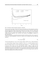
An illustration of the Marching Algorithm is given in Figure 1.
0.2 0.4 0.6 0.8 1.0
x
0.5
1.0
1.5
2.0
v

Fig. 1. Conductivity identification by the Marching Algorithm. The dots are a multiple of the
first eigenfunction at the observation points p
m
. The algorithm identifies the values of the
conductivity a and its discontinuity points
(i) Find l,0
< l < M such that G
l
= max{G
m
: m = 1, 2, ···, M −1} and G
m
< G
l
for any
0
≤ m < l.
(ii) Let i
= 1, m = 0.
(iii) Use Lemma 5.2 to find A
i
, ω
i
and γ
i
from the system
⎧
⎨
⎩
A

i
cos(ω
i
δ −γ
i
)=G
m
,
A
i
cos γ
i
= G
m+1
,
A
i
cos(ω
i
δ + γ
i
)=G
m+2
.
(23)
74
Heat Conduction – Basic Research
Identifiability of Piecewise Constant Conductivity 13
Let
H

i
(x)=A
i
cos(ω
i
(x − p
m+1
)+γ
i
).
(iv) If m
+ 3 ≥ l then go to step (vii). If H
i
(p
m+3
) = G
m+3
,orH
i
(p
m+3
)=G
m+3
and
H

i
(p
m+3
) ≤ 0thena has a discontinuity x

i
on interval [p
m+2
, p
m+3
). Proceed to the next
step (v).
If H
i
(p
m+3
)=G
m+3
and H

i
(p
m+3
) > 0thenletm := m + 1 and repeat this step (iv).
(v) Use Lemma 5.2 to find A
i+1
, ω
i+1
and γ
i+1
from the system
⎧
⎨
⎩
A

i+1
cos(ω
i+1
δ −γ
i+1
)=G
m+3
,
A
i+1
cos γ
i+1
= G
m+4
,
A
i+1
cos(ω
i+1
δ + γ
i+1
)=G
m+5
.
(24)
Let
H
i+1
(x)=A
i+1

cos(ω
i+1
(x − p
m+4
)+γ
i+1
).
(vi) Use formulas in Lemma 5.4 to find the unique discontinuity point x
i
∈ [p
m+2
, p
m+3
).
The parameters and functions used in Lemma 5.4 are defined as follows. Let p
=
p
m+2
, η = δ. To avoid a confusion we are going to use the notation Ω
1
, Ω
2
, Γ
1
, Γ
2
for the corresponding parameters ω
1
, ω
2

, γ
1
, γ
2
required in Lemma 5.4. Let Ω
1
=
ω
i
, Ω
2
= ω
i+1
.Forw(x) use function H
i
(x) recentered at p = p
m+2
,i.e.rewriteH
i
(x)
in the form
w
(x)=H
i
(x)=A cos(Ω
1
(x − p
m+2
)+Γ
1

), |Γ
1
| < π/2.
For v
(x) use function H
i+1
recentered at p + η = p
m+3
,i.e.
v
(x)=H
i+1
(x)=B cos(Ω
2
(x − p
m+3
)+Γ
2
), |Γ
2
| < π/2.
Let i :
= i + 1, m := m + 3. If m < l then return to step (iv). If m ≥ l then go to the next
step (vii).
(vii) Do steps (ii)-(vi) in the reverse direction of x,advancingfromx
= 1tox = p
l+1
.
Identify the values and the discontinuity points of a on
[p

l+1
,1], as well as determine
the corresponding functions H
i
(x).
(viii) Using the notation introduced in (vi) let H
j
(x) be the previously determined function
H on interval
[p
l−2
, p
l−1
]. Recenter it at p = p
l−1
,i.e. w(x)=H
j
(x)=
A cos(Ω
1
(x − p
l−1
)+Γ
1
).LetH
j+1
(x) be the previously determined function H on
interval
[p
l+1

, p
l+2
]. Recenter it at p
l+1
: v(x)=H
j+1
(x)=B cos( Ω
2
(x − p
l+1
)+Γ
2
).If
Ω
1
= Ω
2
then stop, otherwise use Lemma 5.4 with η = 2δ, and the above parameters to
find the discontinuity x
j
∈ [p
l−1
, p
l+1
].Stop.
The justification of the Marching Algorithm is given in (Gutman & Ha, 2007).
6. Identifiability of piecewise constant conductivity with one discontinuity
The Marching Algorithm of Theorem 5.5 requires measurements of the system at possibly
large number of observation points. Our next Theorem shows that if a piecewise constant
conductivity a is known to have just one point of discontinuity x

1
,anditsvaluesa
1
and
a
2
are known beforehand, then the discontinuity point x
1
can be determined from just one
measurement of the heat conduction process.
75
Identifiability of Piecewise Constant Conductivity
14 Will-be-set-by-IN-TECH
Theorem 6.1. Let p ∈ (0, 1) be an observation point, g(x) > 0 on (0, 1), and the observation z
p
(t)=
u(x
p
, t; a), t ∈ (T
1
, T
2
) of the heat conduction process (14) be given. Suppose that the conductivity
a
∈ A
ad
is piecewise constant and has only one (unknown) point of discontinuity x
1
∈ (0, 1).Given
positive values a

1
= a
2
such that a(x)=a
1
for 0 ≤ x < x
1
and a(x)=a
2
for x
1
≤ x < 1 the point
of discontinuity x
1
is constructively identifiable.
Proof. Arguing as in the previous Theorem
z
p
(t)=
∞
∑
k=1
g
k
e
−λ
k
t
ψ
k

(p) ,0≤ T
1
< t < T
2
,
where g
k
= g, ψ
k
 for k = 1, 2, ···.Sinceg
1
ψ
1
(p) > 0 the uniqueness of the Dirichlet series
representation implies that one can uniquely determine the first eigenvalue λ
1
and the value
of G
p
= g
1
ψ
1
(p) .
Without loss of generality one can assume that a
1
> a
2
. In this case we show that the first
eigenvalue λ

1
is strictly increasing as a function of the discontinuity point x
1
∈ [0, 1]. Indeed,
suppose that
0
≤ x
a
1
< x
b
1
≤ 1,
that is
a
(x)=

a
1
,0< x < x
a
1
a
2
, x
a
1
< x < 1
and b
(x)=


a
1
,0< x < x
b
1
a
2
, x
b
1
< x < 1
.
By Theorem 2.2(i)
λ
b
1
=

1
0
b(x)[ψ

1,b
(x)]
2
dx

1
0

[ψ
1,b
(x)]
2
dx
>

1
0
a(x)[ψ

1,b
(x)]
2
dx

1
0
[ψ
1,b
(x)]
2
dx
≥ inf
ψ∈H
1
0
(0,1)

1

0
a(x)[ψ

(x)]
2
dx

1
0
[ψ(x)]
2
dx
= λ
a
1
provided that the derivative ψ

1,b
(x) of the first eigenfunction ψ
1,b
(x) is not identically zero
on
(x
a
1
, x
b
1
).But,from(b(x)ψ


1,b
(x))

= −λ
b
1
ψ
1,b
(x), the assumption ψ

1,b
(x)=0on(x
a
1
, x
b
1
)
implies ψ
1,b
(x)=0on(x
a
1
, x
b
1
). However, this is impossible, since ψ
1,b
(x) > 0on(0, 1).
Thus there exists a unique conductivity of the type sought in the Theorem for which its first

eigenvalue is equal to λ
1
,i.e.a is identifiable.
Now the unique discontinuity point x
1
of a can be determined as follows. Let
ω
1
=

λ
1
a
1
, ω
2
=

λ
1
a
2
.
Then the first eigenfunction ψ
1
is given by
ψ
1
(x)=


A sin ω
1
x,0< x < x
1
,
B sinω
2
(1 −x), x
1
< x < 1
(25)
for some A, B
> 0. The matching conditions at x
1
give
A sin ω
1
x
1
= B sin ω
2
(1 − x
1
) and
A
ω
1
cos ω
1
x

1
=
B
ω
2
cos ω
2
(1 − x
1
).
76
Heat Conduction – Basic Research
Identifiability of Piecewise Constant Conductivity 15
Since ψ
1
(x
1
) > 0wehave0< ω
1
x
1
< π and 0 < ω
2
(1 − x
1
) < π. Therefore x
1
satisfies
1
ω

1
cot ω
1
x =
1
ω
2
cot ω
2
(1 − x).
The existence and the uniqueness of the solution x
1
of the above nonlinear equation follows
from the monotonicity and the continuity of the cotangent functions. Practically, the value of
x
1
can be found by a numerical method.
7. Identifiability with non-zero boundary conditions
Let a ∈PS,andu(x, t; a) be the unique solution of the heat conduction process (4). Next
Theorem describes some conditions under which the identifiability for (4) is possible.
Theorem 7.1. Given σ
> 0 let an integer M be such that
M
≥
3
σ
and M
> 2

μ

ν
.
Suppose that the observations z
m
(t; a)=u(p
m
, t; a) for p
m
= m/M, m = 1, 2, ···, M − 1 and
t
> 0 of the heat conduction process (4) are given. Then the conductivity a ∈ A
ad
is identifiable in the
class of piecewise constant functions
PC(σ) in each one of the following four cases.
(i) f
= 0, q
1
= 0, q
2
= 0, g > 0, g ∈ L
2
(0, 1).
(ii) g
= 0, q
1
= 0, q
2
= 0, f (x , t)=h (x)r(t ) = 0, h > 0, h ∈ L
2

(0, 1), r ∈ C[0, ∞).
(iii) g
= 0, f = 0, q
2
= 0, q
1
= 0, q
1
(0)=0, q
1
∈ C
1
[0, ∞).
(iv) g
= 0, f = 0, q
1
= 0, q
2
= 0, q
2
(0)=0, q
2
∈ C
1
[0, ∞).
Proof. Case (i) is considered in Theorem 5.5. In case (ii) of the Theorem let
y
m
(t)=
∞

∑
k=1
h, ψ
k
ψ
k
(p
m
)e
−λ
k
t
. (26)
Then y
m
(t) is the solution of (4) with g = h, f = 0 and zero boundary conditions, observed
at p
m
∈ (0, 1). It is shown in Theorem 3.2 that such a solution is a continuous function for
t
> 0. Furthermore, using the estimate |ψ
k
(x)|≤
√
λ
k
/
√
ν established in Theorem 3.1, and
the Cauchy-Schwarz inequality we get


∞
0
|y
m
(t)|dt ≤
∞
∑
k=1
1
λ
k
|h
k
||ψ
k
(p
m
)|≤
1
√
ν
∞
∑
k=1
|h
k
|
√
λ

k
≤ Ch < ∞. (27)
Therefore y
m
(t) ∈ L
1
[0, ∞).
Returning to the observation z
m
(t), Theorem 3.2 shows that it is given by
z
m
(t)=u(p
m
, t)=

t
0

∞
∑
k=1
h, ψ
k
ψ
k
(p
m
)e
−λ

k
(t−τ)

r
(τ) dτ.
That is
z
m
(t)=

t
0
y
m
(t −τ)r(τ) dτ.
77
Identifiability of Piecewise Constant Conductivity
16 Will-be-set-by-IN-TECH
Since y
m
(t) ∈ L
1
[0, ∞) and r(t) is continuous and bounded on [0, ∞),TitchmarshTheorem
(Titchmarsh, 1962), Theorem 152, Chap. XI, p. 325, implies that this Volterra integral equation
is uniquely solvable for y
m
(t).
Since h
> 0 is assumed to be in L
2

(0, 1), one has C(a)=h, ψ
1
(a) = 0. The uniqueness of the
Dirichlet series representation (26) and rest of the argument is the same as in the proof of case
(i).
In case (iii) of the Theorem function Φ
(x , t; a) has the form Φ(x, t; a)=q
1
(t)ξ(x; a),where
ξ
(x ; a)=1 −
1

1
0
1
a(s)
ds

x
0
1
a(s)
ds.
Note that ξ
(x ; a) is bounded, continuous and strictly positive on (0, 1).Thusξ ∈ L
2
(0, 1).Let
ξ
k

= ξ(x; a), ψ
k
(x ; a) for k = 1, 2, Then φ
k
(t; a)=q
1
(t)ξ
k
, φ
k
(0; a)=0andφ

k
(t; a)=
q

1
(t)ξ
k
.
Let
y
m
(t)=−
∞
∑
k=1
ξ
k
ψ

k
(p
m
)e
−λ
k
t
. (28)
Arguing as in case (ii), we conclude that y
m
(t) is continuous on [0, ∞) and y
m
(t) ∈ L
1
[0, ∞).
Also, by Theorem 3.2
z
m
(t)=u(p
m
, t)=−

t
0

∞
∑
k=1
ξ
k

ψ
k
(p
m
)e
−λ
k
(t−τ)

q

1
(τ) dτ.
That is
z
m
(t)=

t
0
y
m
(t − τ)q

1
(τ) dτ.
Since y
m
(t) ∈ L
1

[0, ∞) and q

1
(t) is continuous and bounded on [0, ∞),TitchmarshTheorem
(Titchmarsh, 1962), Theorem 152, Chap. XI, p. 325, implies that this Volterra integral equation
is uniquely solvable for y
m
(t).
Since ξ
1
> 0andψ
1
(p
m
) > 0, the uniqueness of the Dirichlet series representation (28)
implies that the M-tuple
G(a) is recoverable from the observations z
m
(t).InthiscaseC(a)=

ξ(x; a), ψ
1
(x ; a). Finally, the Marching Algorithm identifies the unknown conductivity a.
Case (iv) of the Theorem is treated in the same way as case (iii).
8. Continuity of the identification map
The Marching Algorithm establishes the identifiability of the conductivity a ∈PC(σ) from
the data
G(a). In other words, the inverse mapping G
−1
is well defined on G(PC(σ)).To

prove our main result that the identifiability map
G
−1
is continuous, first we show that the
set
PC(σ) ⊂ A
ad
is compact in L
1
(0, 1). A proof of this result can be found in (Gutman & Ha,
2009).
Theorem 8.1. Let A
ad
be equipped with the L
1
(0, 1) topology. Let N ∈ N and σ > 0.Then
(i) Set
PC
N
⊂ A
ad
is compact.
(ii) Set
PC(σ) ⊂ A
ad
is compact.
Theorem 8.2. Let A
ad
be equipped with the L
1

(0, 1) topology, and the data map G : PC(σ) → R
M
be defined as in (3). Then the identifiability map G
−1
: G(PC(σ)) →PC(σ) is continuous.
78
Heat Conduction – Basic Research
Identifiability of Piecewise Constant Conductivity 17
Proof. Theorem 7.1 shows that in every case specified there the data map a →G(a) is defined
everywhere on
PC(σ) and that the conductivity a is identifiable from G(a),i.e.G is invertible
on
G(PC(σ)). By Theorem 8.1 the set PC(σ) is compact in L
1
(0, 1). Thus the Theorem would
be established if the injective map a
→G(a) were shown to be continuous.
Recall that
G(a)=(λ
1
(a), G
1
(a), ···,G
M −1
(a)) ∈ R
M
. The continuity of a → λ
1
(a) was
established in Theorem 4.1. In every case of Theorem 7.1 the data G

m
has the form G
m
(a)=
C(a)ψ
1
(p
m
; a),wherep
m
are the observation points. By Theorem 4.2 the mapping a → ψ
1
(·; a)
is continuous from PC(σ) ⊂ L
1
(0, 1) into C[0, 1]. Thus the evaluation maps a → ψ
1
(p
m
; a) ∈
R are continuous for every p
m
∈ [0, 1].
To see that a
→ C(a) is continuous we have to examine it separately for each case of Theorem
7.1. In case (i) C
(a)=g, ψ
1
(a),whereg ∈ L
2

(0, 1) is a fixed initial condition. The continuity
of the inner product and of a
→ ψ
1
(·; a) imply the continuity of C(a). In case (ii) C(a)=

h, ψ
1
(a) for an h ∈ L
2
(0, 1) and the continuity of C(a) follows. In cases (iii) and (iv) the
continuity of C
(a) is established similarly.
9. Identifiability with a known heat flux
Let Π be the set of piecewise constant functions on [0, 1] with finitely many discontinuity
points,
Π
= {a(x) :0< ν ≤ a(x) ≤ μ, a(x)=a
j
, x ∈ [x
j−1
, x
j
), j = 1, 2, , n} (29)
with x
0
= 0andx
n
= 1.
Consider the following heat conduction problem in an inhomogeneous bar of the unit length

with a conductivity a
∈ Π:
⎧
⎨
⎩
u
t
=(a(x)u
x
)
x
, (x , t) ∈ Q =(0,1) ×(0, ∞),
u
(0, t)=g(t), u(1, t)=0, t ∈ (0, ∞),
u
(x ,0)=0, x ∈ (0, 1).
(30)
Suppose that the extra data f
(t)=a(0)u
x
(0, t) ≡ 0, i.e., the heat flux through the left end of
the bar, is known.
The inverse problem (IP) for (29)-(30) is:
IP: Given f
(t) and g(t) for all t > 0,finda(x).
In this Section we establish the identifiability for the IP. Additional details including a fast
computational algorithm can be found in (Gutman & Ramm, 2010) and (Hoang & Ramm,
2009).
The main idea of the proof is to apply a "layer peeling" argument. Suppose that two
conductivities a, b

∈ Π satisfy (30) with the same data f (t) and g(t) for t > 0. Let both a and
b have no discontinuities on an interval
[0, y],0< y ≤ 1. Then we can show that a(x)=b(x)
for x ∈ [0, y]. A repeated application of this argument shows that a = b on the entire interval
[0, 1]. See (Hoang & Ramm, 2009) for further refinements of this result, in particular for the
data f , g available only on a finite interval
(0, T).
The main tool for the uniqueness proof is Property C (completeness of the products
of solutions for (30)). We will use the following Property C result established in
(Hoang & Ramm, 2009).
Theorem 9.1. Let PC
[0, 1] be the set of piecewise-constant functions on [0, 1].Letq
1
, q
2
∈ PC [0, 1]
be two positive functions. Suppose that ψ
1
(x , k) and ψ
2
(x , k) satisfy
−ψ

j
(x , k)+k
2
q
2
j
(x)ψ

j
(x , k)=0, ψ
j
(1, k)=1, ψ

j
(1, k)=0, j = 1, 2. (31)
79
Identifiability of Piecewise Constant Conductivity
18 Will-be-set-by-IN-TECH
Then the set of products {ψ
1
(x , k)ψ
2
(x , k)}
k>0
is dense in PC[0, 1].Thatis,ifh∈ PC[0, 1] and

1
0
h(x)ψ
1
(x , k)ψ
2
(x , k)dx = 0 (32)
for any k
> 0,thenh= 0.
Theorem 9.2. Problem IP has at most one solution a
∈ Π.
Proof. Following Hoang & Ramm (2009), problem (30) is restated in terms of the Laplace

transform
v
(x , s; a)=(Lu)(x, s; a)=

∞
0
u(x, t; a)e
−st
dt, s > 0.
Let G
(s)=L(g(t)) and F(s)=L( f (t)). Thus (30) with the extra condition a(0)u
x
(0, t)= f (t)
becomes
(a(x)v

)

−sv = 0, 0 < x < 1,
v
(0, s; a)=G(s), a(0)v

(0, s; a)=F(s), (33)
v
(1, s; a)=0.
Let
k
=
√
s, ψ(x, k)=a(x)v


(x , s; a),andq(x)=

1
a(x)
.
Then, using k
2
v(x, s; a)=ψ

(x , k), system (33) is rewritten as
−ψ

(x , k)+k
2
q
2
(x)ψ(x, k)=0, 0 < x < 1, (34)
ψ
(0, k)=F(k
2
), ψ

(0, k)=k
2
G(k
2
), ψ

(1, k)=0.

Let ψ
1
(x , k) and ψ
2
(x , k) be the solutions of (34) for two positive piecewise-constant functions
q
1
(x) and q
2
(x) correspondingly. That is,
−ψ

1
(x , k)+k
2
q
2
1
(x)ψ
1
(x , k)=0, 0 < x < 1, (35)
ψ
1
(0, k)=F(k
2
), ψ

1
(0, k)=k
2

G(k
2
), ψ

1
(1, k)=0,
and
−ψ

2
(x , k)+k
2
q
2
2
(x)ψ
2
(x , k)=0, 0 < x < 1, (36)
ψ
2
(0, k)=F(k
2
), ψ

2
(0, k)=k
2
G(k
2
), ψ


2
(1, k)=0.
Multiply equation (35) by ψ
2
(x , k) and integrate it over [0, 1]. Then use an integration by parts
and the boundary conditions in (35) and (36) to obtain
k
2

1
0
q
2
1
ψ
1
ψ
2
dx = ψ

1
ψ
2
|
1
0
−

1

0
ψ

1
ψ

2
dx = −k
2
G(k
2
)F(k
2
) −

1
0
ψ

1
ψ

2
dx. (37)
Similarly,
k
2

1
0

q
2
2
ψ
1
ψ
2
dx = −k
2
G(k
2
)F(k
2
) −

1
0
ψ

1
ψ

2
dx. (38)
80
Heat Conduction – Basic Research
Identifiability of Piecewise Constant Conductivity 19
Subtracting (38) from (37) gives

1

0
(q
2
1
−q
2
2
)ψ
1
ψ
2
dx = 0
for any k
> 0.
Given nonzero F and G, consider (35) as an initial value problem for ψ
1
at x = 0. Its solution
ψ
1
(x , k) must satisfy ψ
1
(1, k) = 0, because of the condition ψ

1
(1, k)=0. The same goes
for ψ
2
(x , k). Now we can conclude that the set of products {ψ
1
(x , k)ψ

2
(x , k)}
k>0
is dense in
PC
[0, 1] by Theorem 9.1. Therefore q
1
= q
2
. Thus (34) has a unique solution q ∈ PC[0, 1].
Consequently (33) has a unique solution a
∈ Π, and the Theorem is proved.
10. Computational algorithms
The main objective of this research is the development of a theoretical framework for the
parameter identifiability described in previous sections. Nevertheless, from a practical
perspective it is desirable to develop an algorithm for such an identifiability incorporating
the new insights gained in the theoretical part. The main new element of it is the separation
of the identification process into the following two parts. First, the observation data is
used to recover the M-tuple
G(a), i.e. the first eigenvalue of (5), and a multiple of the first
eigenfunction at the observation points p
m
, see (3). In the second step this input is used to
recover the conductivity distribution. We emphasize that only one (first) eigenvalue and the
eigenfunction are needed for the identification. For other methods for inverse heat conduction
problems see (Beck et al., 1985) and the references therein.
Before considering noise contaminated observation data z
m
(t), let us assume that z
m

(t) are
known precisely on an interval I
=(t
0
, T), t
0
≥ 0. In case (i) of Theorem 7.1 the observations
are given by the Dirichlet series
z
m
(t)=
∞
∑
k=1
g , ψ
k
e
−λ
k
t
ψ
k
(p
m
). (39)
We have not implemented yet other cases of Theorem 7.1.
In principle, functions z
m
(t) are analytic for t > 0. Therefore they can be uniquely extended
to

(0, ∞) from I. Then the first eigenvalue λ
1
and the data sequence {G
m
=< g, ψ
1
>
ψ
1
(p
m
)}
M −1
m
=1
can be recovered from the Dirichlet series (39) representing z
m
(t) by
λ
1
= −
1
h
lim
t→∞
ln
z
m
(t + h)
z

m
(t)
, G
m
= lim
t→∞
e
λ
1
t
z
m
(t), (40)
where h
> 0.
The second step of the algorithm, i.e. the identification of the conductivity a is accomplished
by the Marching Algorithm. Numerical experiments show that it provides the perfect
identification only if
G(a) is known precisely. However, even for noiseless data z
m
(t),the
numerical identification of
G(a) from the Dirichlet series (39) representing z
m
(t) can only be
accomplished with a significant error. This numerical evidence is presented in (Gutman & Ha,
2009).
Hence a different algorithm is needed for the practically important case of noise contaminated
data. It should also take into account the severe ill-posedness of the identification of data from
Dirichlet series, see (Acton, 1990). Our numerical experiments confirm that even the second

eigenvalue of the associated Sturm-Liouville problem cannot be reliably identified even for
81
Identifiability of Piecewise Constant Conductivity
20 Will-be-set-by-IN-TECH
noiseless data. It is the distinct advantage of the proposed algorithm that it uses only the
first eigenvalue λ
1
for the conductivity identification. In what follows LMA refers to the
Levenberg-Marquardt algorithm for the nonlinear least squares minimization, and BA to the
Brent algorithm for a single variable nonlinear minimization, see (Press et al., 1992) for details.
First, consider a simple regression type algorithm for the identification of the M-tuple
G(a).
In step 1, for each observation data z
m
(t) we find λ and c to best fit z
m
(t) in the objective
function Ψ
(λ, c; m) defined by (41). In step 2 the obtained eigenvalues λ
(m)
are averaged over
the middle third of the observation points, since such data would presumably be less affected
by noise. The result of the averaging is the sought eigenvalue λ
1
. In step 3, the averaged
eigenvalue λ
1
is kept fixed, and the functions Ψ(λ
1
, c; m) are minimized in variable c only.

The resulting values G
m
form the M-tuple G(a).
Regression Algorithm for λ
1
identification.
Let the data consist of the observations z
m
(t
j
), j = 1,2, J, m = 1,2, ,M −1.
(i) Let λ, c
∈ R and
Ψ
(λ, c; m)=
J
∑
j=1
(ce
−λt
j
−z
m
(t
j
))
2
. (41)
Let
Ψ

(λ, c
m
(λ); m)=min
c∈R
Ψ(λ, c; m).
Note that such a minimizer c
m
(λ) can be found directly by
c
m
(λ)=
∑
J
j
=1
z
m
(j)e
−λt
j
∑
J
j
=1
e
−2λt
j
.
For each m
= 1, ,M − 1 apply BA to find a λ

(m)
such that
Ψ
(λ
(m)
, c
m
(λ
(m)
); m)=min
λ∈R
Ψ(λ, c
m
(λ); m).
(ii) Let k
= card{[[ M/3]], ,[[2M/3]]} and
λ
1
=
1
k
[[2M/3]]
∑
m=[[M/3]]
λ
(m)
1
.
(iii) Keep λ
1

fixed. For each m = 1, ,M −1findG
m
= c
m
(λ
1
) such that
Ψ
(λ
1
, G
m
; m)=min
c∈R
Ψ(λ
1
, c; m).
(iv) Let
G(a)={λ
1
, G
1
, ,G
M −1
}.
One may assume that fitting the data z
m
(t) using two exponents as in (43) could result in
a better estimate for the eigenvalue λ
1

. To examine this assumption let us consider a more
complicated algorithm which we call the LMA Algorithm for λ
1
identification. This algorithm
proceeds as follows (see details below).
82
Heat Conduction – Basic Research
Identifiability of Piecewise Constant Conductivity 21
(i). This step is the same as step (i) in the regression algorithm above, i.e. we minimize the
functions Ψ
(λ, c; m) in both λ and c for m = 1, ,M − 1. Call the minimizers by μ
(m)
and
c
m
(μ
(m)
) respectively.
(ii). Apply the LMA to minimize Φ
(μ, ν, c, b; m) defined in (43). Use the initial guess
μ
(m)
,4μ
(m)
, c
m
(λ),0forthevariablesμ, ν, c, b correspondingly. Call the results of these
minimizations for the variable μ by λ
(m)
1

. The initial value 4μ
(m)
for the second eigenvalue
is used because of Theorem 2.2(iii). A direct application of the LMA without the initial values
obtained in Step (i) did not produce consistent results. Now the data z
m
(t) is approximated
by the first two terms of the Dirichlet series (39). Thus, for each m there is an estimate λ
(m)
1
for
the first eigenvalue λ
1
.
(iii). Let λ
1
be an average of the computed values λ
(m)
1
. We used the middle third of the indices
m since the maximum of our initial data g
(x) was attained in the middle of the interval [0, 1].
Hence these observations were relatively less affected by the noise.
(iv-v). Repeat the minimizations of Steps (i) and (ii), but keep λ
1
frozen. Let G
m
be the values
of the coefficients c that minimize Φ
(λ

1
, ν, c, b; m). This is the best fit to the data z
m
(t) by the
first two terms of the Dirichlet series (39) with the fixed first eigenvalue λ
1
.Bynowthefirst
part of the identification algorithm is completed, since we have recovered the first eigenvalue
λ
1
and a multiple G
m
of the first eigenfunction ψ
1
(p
m
), m = 1,2, ,M −1.
LMA Algorithm for λ
1
identification.
Let the data consist of the observations z
m
(t
j
), j = 1,2, J, m = 1,2, ,M −1.
(i) Let λ, c
∈ R and
Ψ
(λ, c; m)=
J

∑
j=1
(ce
−λt
j
−z
m
(t
j
))
2
. (42)
Let
Ψ
(λ, c
m
(λ); m)=min
c∈R
Ψ(λ, c; m).
Note that such a minimizer c
m
(λ) can be found directly by
c
m
(λ)=
∑
J
j
=1
z

m
(j)e
−λt
j
∑
J
j
=1
e
−2λt
j
.
For each m
= 1, , M −1 apply BA to find a μ
(m)
such that
Ψ
(μ
(m)
, c
m
(μ
(m)
); m)=min
λ∈R
Ψ(λ, c
m
(λ); m).
(ii) Let
Φ

(μ, ν, c, b; m)=
J
∑
j=1
(ce
−μt
j
+ be
−νt
j
−z
m
(t
j
))
2
. (43)
Apply the LMA to minimize Φ
(μ, ν, c, b; m) using the initial guess
μ
(m)
,4μ
(m)
, c
m
(μ
(m)
),0forthevariablesμ, ν, c, b correspondingly. Let
Φ
(λ

(m)
1
, ν
m
, c
m
, b
m
; m)= min
μ,ν,c,b
Φ(μ, ν, c, b; m).
83
Identifiability of Piecewise Constant Conductivity
22 Will-be-set-by-IN-TECH
(iii) Let k = card{[[ M/3]], ,[[2M/3]]} and
λ
1
=
1
k
[[2M/3]]
∑
m=[[M/3]]
λ
(m)
1
.
(iv) Find c
m
(λ

1
), m = 1,2, ,M (asinStep1)suchthat
Ψ
(λ
1
, c
m
(λ
1
); m)=min
c∈R
Ψ(λ
1
, c; m).
(v) Apply the LMA to minimize Φ
(λ
1
, ν, c, b; m) in variables ν, c, b using the initial guess
4λ
1
, c
m
(λ
1
),0forthevariablesν, c, b correspondingly. Let
Φ
(λ
1
, ν
m

, G
m
, b
m
; m)=min
ν,c,b
Φ(λ
1
, ν, c, b; m).
(vi) Let
G(a)={λ
1
, G
1
, ,G
M −1
}.
The second part of the algorithm identifies the conductivity
¯
a from the M-tuple
G(a).As
we have already mentioned the Marching Algorithm provides a perfect identification for
noiseless data, otherwise one has to find
¯
a by a nonlinear minimization.
Identification of piecewise constant conductivity.
The data is the M-tuple G(a)={λ
1
, G
1

, ,G
M −1
}.
(i) Fix N
> 0. Form the objective function Π(a) by
Π
(a)=min
c∈R
M
∑
m=1
(cG
m
−ψ
1
(p
m
; a))
2
, (44)
for the conductivities a
∈ A
N
⊂ A
ad
having at most N − 1 discontinuity points on the
interval
[0, 1].
(ii) Use Powell’s minimization method in K
= 2N −1variables(N −1 discontinuity points

and N conductivity values) to find
Π
(
¯
a
)= min
a∈A
N
Π(a).
The minimizer
¯
a is the sought conductivity.
The function ψ
1
(p
m
; a) in step (i) of the above algorithm is the first normalized eigenfunction
of the Sturm-Liouville problem (5) corresponding to the conductivity a
∈ A
N
. Powell’s
minimization method, a shooting method for the computation of the eigenvalues and the
eigenfunctions, and numerical experiments are presented in (Gutman & Ha, 2009).
11. Conclusions
While in most parameter estimation problems one can hope only to achieve the best fit to
data solution, sometimes it can be shown that such an identification is unique. In such case
it is said that the sought parameter is identifiable within a certain class. In our recent work
(Gutman & Ha, 2007; 2009) we have shown that piecewise constant conductivities a
∈PC(σ)
are identifiable from observations z

m
(t; a) of the heat conduction process (2) taken at finitely
many points p
m
.
84
Heat Conduction – Basic Research
Identifiability of Piecewise Constant Conductivity 23
Let G(a)={λ
1
(a), G
1
(a), ···, G
M −1
(a)}, where he values G
m
(a) are a constant nonzero
multiple of the first eigenfunction ψ
1
(a). In principle, if G(a) is known, then the identification
of the conductivity a can be accomplished by the Marching Algorithm. Theorem 7.1 shows
under what conditions the M-tuple
G(a) can be extracted from the observations z
m
(t),thus
assuring the identifiability of a.
It is shown in Theorem 8.2 that the Marching Algorithm not only provides the unique
identification of the conductivity a, but that the identification is also continuous (stable). This
result is based on the continuity of eigenvalues, eigenfunctions, and the solutions with respect
to the L

1
(0, 1) topology in the set of admissible parameters A
ad
,seeSection4.
Numerical experiments show that, because of the ill-posedness of the identification of
eigenvalues from a Dirichlet series representation, one can only identify
G(a) with some
error. Thus the Marching Algorithm would not be practically useful. In Section 10 we
presented algorithms for the identification of conductivities from noise contaminated data.
Its main novel point is, in agreement with the theoretical developments, the separation of the
identification process into two separate parts. In part one the first eigenvalue and a multiple
of the first eigenfunction are extracted from the observations. In the second part a general
minimization method is used to find a conductivity which corresponds to the recovered
eigenfunction.
The first eigenvalue and the eigenfunction in part one of the algorithm are found from the
Dirichlet series representation of the solution of the heat conduction process. The numerical
experiments in (Gutman & Ha, 2009) confirm that even for noiseless data the second
eigenvalue cannot be reliably found. These experiments showed that in our tests a simple
regression type algorithm identified λ
1
better than a more complex Levenberg-Marquardt
algorithm. The last part of the algorithm employs Powell’s nonlinear minimization method
because it does not require numerical computation of the gradient of the objective function.
The numerical experiments show that the conductivity identification was achieved with a
15-18% relative error for various noise levels in the observations.
12. References
Acton, F. S. (1990). Numerical methods that work. Rev. and updated ed., Washington: The
Mathematical Association of America.
Beck, J. V., Blackwell, B. & Clair, C. R. (1985). Inverse heat conduction. Ill-posed problems.,A
Wiley-Interscience Publication. New York etc.: John Wileyand Sons, Inc. XVII.

Benabdallah, A., Dermenjian, Y. & Rousseau, J. L. (2007). Carleman estimates for the
one-dimensional heat equation with a discontinuous coefficient and applications
to controllability and an inverse problem, Journal of Mathematical Analysis and
Applications 336(2): 865 – 887.
Birkhoff, G. & Rota, G C. (1978). Ordinary Differential Equations, 3rd edn, Wiley, New York.
Cannon, J. R. (1984). The one-dimensional heat equation. Foreword by Felix E. Browder.,
Encyclopedia of Mathematics and Its Applications, Vol. 23. Menlo Park, California
etc.: Addison-Wesley Publishing Company; Cambridge etc.: Cambridge University
Press.
Courant, R. & Hilbert, D. (1989). Methods of mathematical physics. Volume I. Transl. and rev.
from the German Original. Reprint of the 1st Engl. ed. 1953., Wiley Classics Edition; A
Wiley-Interscience Publication. New York etc.: John Wiley & Sons.
Demir, A. & Hasanov, A. (2008). Identification of the unknown diffusion coefficient in a linear
parabolic equation by the semigroup approach, Journal of Mathematical Analysis and
Applications 340(1): 5 – 15.
85
Identifiability of Piecewise Constant Conductivity
24 Will-be-set-by-IN-TECH
Duchateau, P. (1995). Monotonicity and invertibility of coefficient-to-data mappings for
parabolic inverse problems, SIAM Journal on Mathematical Analysis 26(6): 1473–1487.
URL: />Elayyan, A. & Isakov, V. (1997). On uniqueness of recovery of the discontinuous conductivity
coefficient of a parabolic equation, SIAM Journal on Mathematical Analysis 28(1): 49–59.
URL: />Evans, L. C. (2010). Partial differential equations. 2nd ed., Graduate Studies in Mathematics 19.
Providence, RI: American Mathematical Society.
Gelfand, I. M. & Levitan, B. M. (1955). On the determination of a differential equation from its
spectral function, Amer. math. Soc. Transl. Ser. 2(2): 253–304.
Gutman, S. & Ha, J. (2007). Identifiability of piecewise constant conductivity in a heat
conduction process, SIAM Journal on Control and Optimization 46(2): 694–713.
URL: />Gutman, S. & Ha, J. (2009). Parameter identifiability for heat conduction with a boundary
input., Math. Comput. Simul. 79(7): 2192–2210.

Gutman, S. & Ramm, A. G. (2010). Inverse problem for a heat equation with
piecewise-constant conductivity, J. Appl. Math. and Informatics 28(3–4): 651–661.
Hoang, N. S. & Ramm, A. G. (2009). An inverse problem for a heat equation with
piecewise-constant thermal conductivity, Journal of Mathematical Physics 50(6): 063512.
URL: />Isakov, V. (2006). Inverse problems for partial differential equations. 2nd ed., Applied Mathematical
Sciences 127. New York, NY: Springer.
Kitamura, S. & Nakagiri, S. (1977). Identifiability of spatially-varying and constant parameters
in distributed systems of parabolic type., SIAM J. Control Optimization 15: 785–802.
Kohn, R. V. & Vogelius, M. (1985). Determining conductivity by boundary measurements ii.
interior results, Communications on Pure and Applied Mathematics 38(5): 643–667.
URL: />Lions, J. (1971). Optimal control of systems governed by partial differential equations. ,
Berlin-Heidelberg-New York: Springer-Verlag.
Nakagiri, S i. (1993). Review of Japanese work of the last ten years on identifiability in
distributed parameter systems., Inverse Probl. 9(2): 143–191.
Orlov, Y. & Bentsman, J. (2000). Adaptive distributed parameter systems identification with
enforceable identifiability conditions and reduced-orderspatial differentiation., IEEE
Trans. A utom. Control 45(2): 203–216.
Pierce, A. (1979). Unique identification of eigenvalues and coefficients in a parabolic problem.,
SIAM J. Control Optimization 17: 494–499.
Press, W. H., Teukolsky, S. A., Vetterling, W. T. & Flannery, B. P. (1992). Numerical recipes in
FORTRAN. The art of scientific computing. 2nd ed., Cambridge: Cambridge University
Press.
Ramm, A. G. (2005). Inverse Problems. Mathematical and analytical techniques with applications to
engineering.,NewYork,NY:Springer.
Saks, S. & Zygmund, A. (1965). Analytic functions, Warsaw: PWN - Polish Scientific Publishers.
IX.
Titchmarsh, E. (1962). Introduction to the theory of Fourier integrals, Oxford University Press.
86
Heat Conduction – Basic Research
4

Experimental and Numerical
Studies of Evaporation Local
Heat Transfer in Free Jet
Hasna Louahlia Gualous
Caen Basse Normandie University/LUSAC
France
1. Introduction
Jet impingement heat transfer has been used extensively in many industrial applications for
cooling because it provides high local heat transfer coefficients at low flow rates. Several
experimental and theoretical studies on liquid jet impingement heat transfer have been
reported in the literature (Louahlia & Baonga, 2008, Chen et al., 2002, Lin & Ponnappan,
2004, Liu & Zhu, 2004, Pan & Webb, 1995). Numerous studies are conducted in average heat
transfer, but local heat transfer analysis for steady and unsteady states has not been much
attention. Jet impingement heat transfer is influenced by different physical parameters such
as: (i) the velocity turbulent fluctuations (Oliphant et al. 1998, Stevens & Webb, 1989), (ii) the
difference between the temperatures of inlet jet and heat exchange surface (Siba et al. 2003,
MA et al. 1997), (iii) the surface geometry and the jet orientation (MA et al. 1997b, Elison &
Webb, 1994), (iv) the liquid flow rate and Prandtl number (Elison & Webb, 1994, Fabbri et al.
2003, Stevens & Webb, 1993), and (v) the nozzle diameter (Stevens & Webb, 1993, 1992).
2. Hydrodynamic characteristics of the jet impinging on a horizontal surfarce
When a liquid jet impinges on a horizontal surface, three distinct regions can be identified as
shown in Figure 1. The first zone is the free jet region where the flow is accelerated because
of the gravitational force. The second zone is the impingement region where the interaction
between the jet and the heat exchange surface produces a strong deceleration of the flow.
After this zone, the liquid wets the surface and flows in a parallel direction to the heat
exchange surface. Heat transfer efficiency in each zone is related to the flow velocity and its
structure. In the impingement zone, jet diameter could be measured using flurescence
induced laser (Baonga et al. 2006) combined to the images processing. In this method, liquid
impinging the heat exchange surface is illuminated by a laser sheet in the axial direction as
shown by Figure 2. Rhodamine B with low concentration must be used as the fluerescent

substance added to the liquid jet. In this case, fluorescent substance becomes visible when
liquid jet is illuminated with light. A CCD camera can be used to record the flow video
images. Video images are treated in order to extract the profiles of the jet as shown by
Figure 1.

Heat Conduction – Basic Research

88
Height [m]

0
0.001
0.002
0.003
0.004
0.005
0.006
-25 -15 -5 5 15 25
Impingement zone
Free jet regime
Parallel flow
N
ozz
l
e
Hydraulic jump
dis
k
Water
z

0
U
j
V
j
r [mm]

Fig. 1. Schematic of flow developing from nozzle to heated disk.

Laser
Laser sheet
Head tank
Test sample
Camera

Fig. 2. Flow visualization system.
2.1 Axial flow structure
For inlet Reynolds number ranging from 1520 to 5900 (the corresponding values of the inlet
mean velocity are in the range of 3.24 to 12.5 m/s), Figure 3 shows effect of the jet flow rate
on the distribution of the jet diameter along the axial direction. The nozzle diameter is of
4 mm. The nozzle-heat exchange surface spacing is of 13 mm. Reynolds number is
calculated as follow :

iL
4m
Re
d





(1)
where: d
i
is the inner diameter of the nozzle,
L

is the dynamic viscosity, m

is the total
mass flow rate of the jet. Physical properties are used at the inlet jet temperature measured
at the nozzle exit.