Advanced Biomedical Engineering Part 11 ppt

Image Processing Methods for Automatic
Cell Counting In Vivo or In Situ Using 3D Confocal Microscopy

191
2.4.2 Apoptotic cells
The typical histogram h(q), where q is the grey level intensity, of median-filtered Caspase
images is composed of two modes, the first one corresponding to the background and the
second one to the sample. There isn’t a third mode that would belong to the apoptotic cells,
due to the very small number of pixels belonging to them. In some Caspase images, the
histogram becomes unimodal, when the background is so low as to disappear, and images
only include the sample.
The following thresholding method was developed. The shape of the second mode,
corresponding to the sample, can be roughly approximated to a Gaussian function G(q), and
the pixels belonging to the Caspase cells are considered outliers. The highest local maximum
of the histogram serves to identify the sample mode. To identify the outliers, assuming the
sample’s pixel grey level intensities are normally distributed, the Gaussian function G
b
(q)
that best fits the shape of the sample’s mode is found. This is achieved by minimizing the
square error between the histogram h(q) in the interval corresponding to the mode and G(q),
that is

min max
() ar
g
min ( )
c
b
qqq
G q error q






(3)
where

max
2
() [ () ()]
c
q
q
error q G q h q

(4)
and

2
2
()
2()
()
qq
q
Gq e






(5)

(q) and

(q) are the mean and standard deviation of the mode respectively, calculated in
the interval [q, q
max
], given by

max
max
()
()
()
c
c
q
qq
q
qq
hqq
q
hq







max
max
2
()( )
()
()
c
c
q
qq
q
qq
hq q
q
hq








(6)
q
c
is a cut-off value given by the global minimum between the first and the second modes, if
the histogram is bimodal, or the first local minimum of the histogram, if it is unimodal, and
q

max
is the maximum grey level of the histogram. The threshold is obtained from the standard
score (z-score), which rejects the outliers of the Gaussian function. The z-score is given by

()
b
b
q
z




(7)
where

b
and

b
are the mean and standard deviation of the best Gaussian function
respectively and q is pixel intensity. It is considered that a grey level is an outlier if z3,
therefore the threshold t is given by

Advanced Biomedical Engineering

192

3t
bb





(8)
2.4.3 Mitotic and glial cells
In images stained with either pH3 or Repo in Drosophila embryos, the mode corresponding to
the cells is almost imperceptible due to the corresponding small number of pixels compared to
the number of background pixels. Given the low number of foreground pixels the histogram
can be considered unimodal. To binarise unimodal images, rather than using thresholding
techniques, we assumed that the background follows a Gaussian distribution G(q) and
considered the pH3 cells outliers. To identify the best Gaussian function, we minimised the
square error in the histogram h(q) in the interval between the mode and threshold, given by

3
bb
t




(10)
following the same procedure employed to threshold apoptotic cells explained before.
2.5 Post-processing
After segmentation, or in parallel, other methods can also be developed to reduce remaining
noise, to separate abutting cells and to recover the original shape of the objects before the
classification. Which method is used will depend on the object to be discriminated.
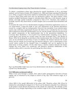
2.5.1 Filtering
Some raw Caspase images have small spots of high intensity, which can be confused with cells
in later steps of the process. To eliminate these spots without affecting the thresholding

technique (if the spot filter is applied before thresholding the histogram is modified affecting
the result), the raw images are filtered in parallel and the result is combined with the
thresholding outcome. If a square window of side greater than the diameter of a typical spot,
but smaller than the diameter of a cell, is centered in a cell, the mean of the pixel intensities
inside the window should be close to the value of the central pixel. If the window is centered
in a spot, the pixel mean should be considerably lower than the intensity of the central pixel.
To eliminate the spots, a mobile window W is centered in each pixel. Let p(x,y) and s(x,y) be the
original input image and the resulting filtered image respectively, and m(x,y) the average of
the intensities inside the window centered in (x,y). If m(x,y) is lower than a certain proportion

with respect to the central pixel, it becomes black, otherwise it retains its intensity. That is

0if (,)(,)
(,)
(,) if (,) (,)
mxy pxy
sxy
p
xy mxy pxy








(11)
where

,
(,) (,)
xy W
mxy pxy



(12)
After thresholding, cells and small spots appear white, while after spot filtering the spots
appear black. The result from both images is combined using the following expression:

0 if min[ ( , ), ( , )] 0
(,)
1 if min[ ( , ), ( , )] 0
txy sxy
qxy
txy sxy






(13)
where q(x, y) is the resulting image and t(x, y) the image resulting form thresholding.
Image Processing Methods for Automatic
Cell Counting In Vivo or In Situ Using 3D Confocal Microscopy

193
The combination of filtering and thresholding results in separating candidate objects

(Caspase-positive cells) from background. The spot filter also separates cells that appear
very close in the z-axis.
To render the Caspase-positive cells more similar in appearance to the original raw images,
three-dimensional morphological operations are then performed throughout the whole
stack. Firstly, morphological closing followed by opening are applied to further remove
noise and to refine the candidate structures. Secondly, the objects containing holes are filled
with foreground colour verifying that each hole is surrounded by foreground pixels.
2.5.2 Cell separation
Cells that appear connected must be separated. This is most challenging. Several automatic
and semi-automatic methods deal with the problem of how to separate cells within clusters
in order to recognise each cell. Initially some seeds or points identifying each cell are found.
A seed is a small part of the cell, not connected to any other, that can be used to mark it. If
more than one seed is found per cell, it will be subdivided (i.e. over-segmentation), but if no
seed is found the cell will not be recognised. In some semiautomatic methods seeds are
marked by hand. Several methods have been proposed to identify only one seed per cell
avoiding over-segmentation. The simplest method consists of a seeding procedure
developed during the preparation of the samples to avoid overlaps between nuclei (Yu et
al., 2009). More practical approaches involve morphological filters (Vincent, 1993) or
clustering methods (Clocksin, 2003; Svensson, 2007). Watershed based algorithms are
frequently employed for contour detection and cell segmentation (Beucher & Lantuejoul,
1979; Vincent & Soille, 1991), some employing different distance functions to separate the
objects (Lockett & Herman, 1994; Malpica, 1997). In this way, cells are separated by defining
the watershed lines between them. Hodneland et al. (Hodneland, 2009) employed a
topographical distance function and Svensson (Svensson, 2007) presented a method to
decompose 3D fuzzy objects, were the seeds are detected as the peaks of the fuzzy distance
transforms. These seeds are then used as references to initiate a watershed procedure. Level
set functions have been combined with watershed in order to reduce over-segmentation and
render the watershed lines more regular. In the method developed by Yu et al. (Yu et al.,
2009) the dynamic watershed is constrained by the topological dependence in order to avoid
merged and split cell segments. Hodneland et al. (Hodneland, 2009) also combine level set

functions and watershed segmentation in order to segment cells, and the seeds are created
by adaptive thresholding and iterative filling. Li et al. propose a different approach, based
on gradient flow tracking (Li et al. 2007, 2008). These procedures can produce good results
in 2D, although they are generally time consuming. They do not provide good results if the
resolution of the images is low and the borders between the cells are imperceptible.
Watershed and h-domes are two morphological techniques commonly used to separate
cells. These two techniques are better understood if 2D images or 3D stacks are seen as a
topological relief. In the 2D case the height in each point is given by the intensity of the pixel
in that position where the cells are viewed as light peaks or domes separated by dark valleys
(Vincent, 1993). The basic idea behind watershed consists in imaging a flooding of the
image, where the water starts to flow from the lower points of the image. The edges
between the regions of the image tend to be placed on the watershed. Frequently, the
watershed is applied to the gradient of the image, so the watershed is located in the crests,
i.e. in the highest values. Watershed and domes techniques are also applied on distance
images. In this way, each pixel or voxel of an object takes the value of the minimum distance

Advanced Biomedical Engineering

194
to the background, and the highest distance will correspond to the furthest point from the
borders. The cells are again localized at the domes of the mountains, while the watershed is
used to find the lowest points in the valleys that are used to separate the mountains, i.e. the
cells (Malpica et al., 1997). In this way, watershed can be used to divide joined objects, using
the inverted of the distance transformation and flooding the mountains starting from the
inverted domes that are used as seeds or points from where the flooding begins. The eroded
points and the resulting points of a top-hat transformation can also be used as seeds in
several watershed procedures.
2.5.2.1 Apoptotic cells
The solution to the cell separation problem depends on the shape of the cells and how close
they are. Apoptotic cells, for example, do not appear very close, although it is possible to

find some abutting one another. They can also have a very irregular shape and can appear
subdivided. Therefore, we reached a compromise when trying to separate cells. When
watershed was used in 3D many cells were subdivided resulting in a cell being counted as
multiple cells, thus yielding false positives. On the other hand, if a technique to subdivide
cells is not used, abutting cells can be counted only as one, yield false negatives. In general,
if there are few abutting cells, the number of false negatives is low. A compromise solution
was employed. Instead of using a 3D watershed, a 2D watershed starting from the last
eroded points was used, thus separating objects in each plane. In this way, irregular cells
that were abutting in one slice were separated, whilst they were kept connected in 3D. The
number of false negatives was reduced without increasing the number of false positives.
Although some cells can still be lost, this conservative solution was found to be the best
compromise.
2.5.2.2 Mitotic and glial cells
Mitotic and glial cells in embryos were separated by defining the watershed lines between
them. To this end, the first step consisted in marking each cell with a seed. In order to find
the seeds a 3D distance transformation was applied. To mark the cells, we applied a 3D h-
dome operator based on a morphological gray scale reconstruction (Vincent, 1993). We
found h = 7 to be the standard minimum distance between the centre of a cell and the
surrounding voxels. This marked all the cells, even if they were closely packed. To avoid a
cell having more than one seed, we found the h-domes transform of an image q(x,y). A
morphological reconstruction of q(x,y) was performed by subtracting from q(x,y)-h, where h
is a positive scalar, the result of the reconstruction from the original image (Vincent, 1992,
1993), that is

h
D (q(x,y)) = q(x,y)
ρ
(q(x,y) h)

 (14)

where the reconstruction

h)y)ρ(q(x,

(15)
is also known as the h-maxima transform. The h extended-maxima, i.e. the regional maxima
of the h-maxima transform, can be employed to mark the cells (Vincent, 1993; Wählby 2003,
Wählby et al. 2004). However, we found that a more reliable identification of the cells that
prevented losing cells, was achieved by the binarisation method of thresholding the h-
domes images (Vincent, 1993). Given that each seed is formed of connected voxels, 3D
domes could be identified and each seed labelled with 18-connectivity.
Image Processing Methods for Automatic
Cell Counting In Vivo or In Situ Using 3D Confocal Microscopy

195
Due to the intensity variation of the cells, several seeds can be found in one cell, resulting in
over-segmentation. To prevent over-segmentation after watershed, redundant seeds must
be eliminated, to result in only one seed per cell. Wählby et al. (Wählby et al., 2004) have
used the gradient among the seeds as a way to determine if two seeds belong to a single cell
and then combine them. However, we found that for mitotic cells a simpler solution was
successful at eliminating excess seeds. Multiple seeds can appear in one cell if there are
irregularities in cell shape. The resulting extra peaks tend not to be very high and, when
domes are found, they tend to occupy a very small number of voxels (maximum of 10).
Instead, true seeds are formed of a minimum of 100 voxels. Consequently, rejecting seeds of
less than 20 voxels eliminated most redundant seeds.
Recently, Cheng and Rajapakse (Cheng and Rajapakse, 2009) proposed an adaptive h
transform in order to eliminate undesired regional minima, which can provide an
alternative way of avoiding over-segmentation. Following seed identification, the 3D
watershed employing the Image Foresting Transform (IFT) was applied (Lotufo & Falcao,
2000; Falcao et al., 2004), and watershed separated very close cells.

2.5.2.3 Neuronal nuclei
To identify the seeds in images of HB9 labelled cells, a 2D regional maxima detection was
performed and following the method proposed by Vincent (Vincent, 1993), a h-dome
operator based on a morphological gray scale reconstruction was applied to extract and
mark the cells. The choice of h is not critical since a range of values can provide good
results (Vincent, 1993). The minimum difference between the maximum grey level of the
cells and the pixels surrounding the cells is 5. Thus, h=5 results in marking cells, while
distinguishing cells within clusters. Images were binarised by thresholding the h-domes
images.
Some nuclei were very close. As we did with the mitotic cells, a 3D watershed algorithm
could be employed to separate them. However in our tests the results were not always good.
We found better and more time-computing efficient results from employing both the
intensity and the distance to the borders as parameters to separate nuclei. In this way, first a
2D watershed was applied to separate nuclei in 2D, based on the intensity of the particles.
Subsequently, 3D erosion was used in order to increase their separation and a 3D distance
transformation was applied. In this way each voxel of an object takes the value of the
minimum distance to the background. Then the 3D domes were found and used as seeds to
mark every cell. A fuzzy distance transform (Svensson, 2007), which combines the intensity
of the voxels and the distance to the borders, was also tested. Whilst with our cells this did
not work well, it might be an interesting alternative with different kinds of cells when
working with other kinds of cells. The images were then binarised. Once the seeds were
found, they were labelled employing 18-connectivity and from the seeds a 3D region
growing was done to recover the original shape of each object, using as mask the stack
resulting from the watershed (see Forero et al, 2010).
2.6 Classification
The final step is classification, whereby cells are identified and counted. This step is done
according to the characteristics that allow to identify each cell type and reject other particles.
A 3D labelling method (Lumia, 1983; Thurfjell, 1992; Hu, 2005) is first employed to identify
each candidate object, which is then one by one either accepted or rejected according to the
selected descriptors. To find the features that better describe the cells, a study of the best

Advanced Biomedical Engineering

196
descriptors must be developed. Several methods are commonly employed to do this. Some
methods consider that descriptors follow a Gaussian distribution, and use the Fisher
discriminant to separate classes (Fisher, 1938; Duda et al., 2001). Other methods select the
best descriptors after a Principal Components Analysis (Pearson, 1901; Duda, 2001). In this
method, a vector of descriptors is obtained for each sample and then the principal
components are obtained. The descriptors having the highest eigen values, that is, those
having the highest dispersion, are selected as best descriptors. It must be noted that this
method can result on the selection of bad descriptors when the two classes have a very high
dispersion along a same principal component, but their distribution overlaps considerably.
In this case the descriptor must be rejected.
In our case, we found that dying cells stained with Caspase and mitotic cells with pH3·are
irregular in shape. Therefore, they cannot be identified by shape and users distinguish them
from background spots of high intensity by their bigger size. Thus, apoptotic and mitotic
cells were selected among the remaining candidate objects from the previous steps based
only on their volume. The minimum volume can be set empirically or statistically making it
higher than the volume occupied by objects produced by noise and spots of high intensity
that can still remain. The remaining objects are identified as cells and counted. Using
statistics, a sufficient number of cells and rejected particles can be obtained to establish their
mean and standard deviation, thus finding the best values that allow to separate both
classes using a method like the Fisher discriminator.
Nuclei have a very regular, almost spherical, shape. In this case more descriptors can be
used to better describe cells and get a better identification of the objects. 2D and 3D
descriptors can be employed to analyse the objects. Here we only present some 2D
descriptors. For a more robust identification the representation of cells should preferably be
translation, rotation and scale invariant. Compactness, eccentricity, statistical invariant
moments and Fourier descriptors are compliant with this requirement. We did not use

Fourier descriptors for our studies given the tiny size of the cells, which made obtaining
cells’ contours very sensitive to noise. Therefore, we only considered Hu’s moments,
compactness and eccentricity.
Compactness C is defined as

2
P
C
A
 (16)
where A and P represent the area and perimeter of the object respectively. New 2D and 3D
compactness descriptors to analyse cells have been introduced by Bribiesca (2008), but have
not been tested yet.
Another descriptor corresponds to the flattening or eccentricity of the ellipse, whose
moments of second order are equal to those of the object. In geometry texts the eccentricity
of an ellipse is defined as the ratio between the foci length a and the major axis length D of
its best fitting ellipse

a
E
D

(16)
Its value varies between 0 and 1, when the degenerate cases appear, being 0 if the ellipse is
in fact a circumference and 1 if it is a line segment. The relationship between the focal length
and the major and minor axes, D and d respectively, is given by the equation
Image Processing Methods for Automatic
Cell Counting In Vivo or In Situ Using 3D Confocal Microscopy

197

D
2
=d
2
+a
2
(17)
then,

22
Dd
E
D



(18)

Nevertheless, some authors define the eccentricity of an object as the ratio between the
length of the major and minor axes, also being named aspect ratio, and elongation because it
quantifies the extension of the ellipse and is given by

2
1
d
eE
D
 
(19)
In this case, eccentricity also varies between 0 and 1, but being now 0 if the object is a line

segment and 1 if it is a circumference.
The moment invariants are obtained from the binarised image of each cell; pixels inside the
boundary contours are assigned to value 1 and pixels outside to value 0. The central
moments are given by:

11
00
()()(,)
NM
rs
rs
xy
xx yyfxy





for r, s = 0, 1, …, ∞ (20)
where f(x,y) represents a binary image, p and q are non-negative integers and (
x , y ) is the
barycentre or centre of gravity of the object and the order of the moment is given by r + s.
From the central moments Hu (Hu, 1962) defined seven rotation, scale and translation
invariant moments of second and third order

12002
22
22002 11
22
330 12 2103

22
43012 2103
22
5 30 123012 3012 2103
22
21 03 21 03 30 12 21 03
2
620023012 21
()4
(3)(3 )
()()
(3)( )( )3( )
(3 )( ) 3( ) ( )
()()(


 
  
 
   
  
  

 
  
 

     



 

  
2
03 11 30 12 21 03
22
7210330123012 2103
22
12 30 21 03 30 12 21 03
)4( )( )
(3 )( ) ( ) 3( )
(3 )( ) 3( ) ( )

   
 
  

  


   


 


(21)
Moments 
1
to 

6
are, in addition, invariant to object reflection, given that only the
magnitude of 
7
is constant, but its sign changes under this transformation. Therefore, 
7
can
be used to recognize reflected objects. As it can be seen from the equations, the first two
moments are functions of the second order moments. 
1
is function of

20
and

02
, the
moments of inertia of the object with respect to the coordinate axes x and y, and therefore
corresponds to the moment of inertia, measuring the dispersion of the pixels of the object

Advanced Biomedical Engineering

198
with respect to its centre of mass, in any direction. 
2
indicates how isotropic or directional
the dispersion is.
One of the most common errors in the literature consists of the use of the whole set of Hu’s
moments to characterise objects. They must not be used simultaneously since they are
dependant (Flusser, 2000), given that

5
22
7
3
3
4






(22)
Since Hu’s moments are not basis (meaning by a basis the smallest set of invariants by
means of which all other invariants can be expressed) given that they are not independent
and the system formed by them is incomplete, Flusser (2000) developed a general method to
find bases of invariant moments of any order using complex moments. This method also
allows to describe objects in 3D (Flusser et al, 2009).
As cells have a symmetrical shape, the third and higher odd order moments are close to
zero. Therefore, the first three-order Hu’s moment
3

is enough to recognize symmetrical
objects, the others being redundant.
That is, eccentricity can be also derived from Hu’s moments by:

12
12
e








(23)
and, from Equation (19) it can be found that:

2
2
12
2
1
Ee





(24)
Therefore, eccentricity
is not independent of the first two Hu’s moments and it must not be
employed simultaneously with these two moments for classification.
3. Conclusion
We have presented here an overview of image processing techniques that can be used to
identify and count cells in 3D from stacks of confocal microscopy images. Contrary to
methods that count automatically dissociated cells or cells in culture, these 3D methods
enable cell counting in vivo (i.e. in intact animals, like Drosophila embryos) and in situ (i.e.

in a tissue or organ). This enables to retain normal cellular context within an organism. To
give practical examples, we have focused on cell recognition in images from fruit-fly
(Drosophila) embryos labelled with a range of cell markers, for which we have developed
several image-processing methods. These were developed to count apoptotic cells stained
with Caspase, mitotic cells stained with pH3, neuronal nuclei stained with HB9 and glial
nuclei-stained with Repo. These methods are powerful in Drosophila as they enable
quantitative analyses of gene function in vivo across many genotypes and large sample
sizes. They could be adapted to work with other markers, with stainings of comparable
qualities used to visualise cells of comparable sizes (e.g. sparsely distributed nuclear labels
like BrdU, nuclear-GFP, to count cells within a mosaic clone in the larva or adult fly).
Image Processing Methods for Automatic
Cell Counting In Vivo or In Situ Using 3D Confocal Microscopy

199
Because automatic counting is objective, reliable and reproducible, comparison of cell
number between specimens and between genotypes is considerably more accurate with
automatic programs than with manual counting. While a user normally gets a different
result in each measurement when counting manually, automatic programs obtain
consistently a unique value. Thus, although some cells may be missed, since the same
criterion is applied in all the stacks, there is no bias or error. Consistent and objective criteria
are used to compare multiple genotypes and samples of unlimited size. Furthermore,
automatic counting is considerably faster and much less labour intensive.
Following the logical steps explained in this review, the methods we describe could be
adapted to work on a wide range of tissues and samples. They could also be extended and
combined with other methods, for which we present an extended description, as well as
with some other recent developments that we also review. This would enable automatic
counting in vivo from mammalian samples (i.e. brain regions in the mouse), small
vertebrates (e.g. zebra-fish) or invertebrate models (e.g. snails) to investigate brain structure,
organism growth and development, and to model human disease.
4. References

Adiga, P.U. & Chaudhuri B. (2001). Some efficient methods to correct confocal images for
easy interpretation.
Micron, Vol. 32, No. 4, (June 2001), pp. 363-370, ISSN 09684328
Anscombe, F. J. (1948). The transformation of Poisson, Binomial and Negative-Binomial
data.
Biometrika, Vol. 35, No. 3/4, (December 1948), pp. 246-254, ISSN 00063444
Bar-Lev, S.K. & Enis, P. (1988). On the classical choice of variance stabilizing transformations
and an application for a Poisson variate.
Biometrika, 1988, Vol. 75, No. 4, (December
1988), pp. 803-804, ISSN 00063444
Bello B.C., Izergina N., Cussinus E. & Reichert H. (2008). Amplification of neural stem cell
proliferation by intermediate progenitor cells in Drosophila brain development.
Neural Development, Vol. 3, No. 1, (February 2008), pp. 5, ISSN 17498104
Bello B, Reichert H & Girth F. (2006). The brain tumor gene negatively regulates neural
progenitor cell proliferation in the larval central brain complex of Drosophila.
Development, Vol. 133, No. 14, (July 2006), pp. 2639-2648, ISSN 10116370
Beucher, S. & Lantuejoul, C. (1979). Use of watersheds in contour detection
International
workshop on image processing: Real-time and motion detection/estimation. IRISA,
(September 1979), Vol. 132, pp. 2.1-2.12
Bribiesca, E. (2008). An easy measure of compactness for 2D and 3D shapes.
Pattern
Recognition.
Vol. 41, No. 2, (February 2008), pp. 543-554, ISSN 0031-3203
Calapez, A. & Rosa, A. (2010). A statistical pixel intensity model for segmentation of
confocal laser scanning microscopy images.
IEEE Transactions on Image Processing,
Vol. 19, No. 9, (September 2010), pp. 2408-2418, ISSN 10577149
Can, A. et al. (2003). Attenuation correction in confocal laser microscopes: A novel two-view
approach.

Journal of Microscopy, Vol. 211, No. 1, (July 2003), pp. 67-79, ISSN
00222720
Carpenter AE et al. (2006). CellProfiler: image analysis software for identifying and
quantifying cell phenotypes
Genome Biology, Vol. 7, No. 10, (October 2006), Article
R1000, ISSN 14656906

Advanced Biomedical Engineering

200
Chan, T. F.; Sandberg, B. Y. & Vese, L. A. (2000). Active contours without edges for vector-
valued images.
Journal of Visual Communication and Image Representation. Vol. 11,
No. 2, (February 2000), pp. 130-141, ISSN 10473203
Chan, T. & Vese, L. (2001). Active contours without edges.
IEEE Transactions on Image
Processing
. Vol 10, No. 2, (February 2001), pp. 266-277, ISSN 10577149
Cheng, J. & Rajapakse, J. (2009). Segmentation of clustered nuclei with shape markers and
marking function,
IEEE Transactions on Biomedical Engineering, Vol. 56, No. 3,
(March 2009), pp. 741-748, ISSN 00189294
Clocksin, W. (2003). Automatic segmentation of overlapping nuclei with high background
variation using robust estimation and flexible contour models.
Proceedings 12th
International Conference on Image Analysis and Processing
, pp. 682-687, ISBN
0769519482, Mantova, Italy, September 17-19, 2003
Conchello, J.A. (1995). Fluorescence photobleaching correction for expectation maximization
algorithm.

Three-Dimensional microscopy: image acquisition and processing. Proceedings
of the 1995 SPIE symposium on electronic imaging: Science and technology.
Wilson, T. &
Cogswell C. J. (Eds.). Vol. 2412, pp. 138-146, ISBN 9780819417596, March 23, 1995
Dima, A.; Scholz, M. & Obermayer, K. (2002). Automatic segmentation and skeletonization
of neurons from confocal microscopy images based on the 3-D wavelet transform.
IEEE Transactions on Image Processing, 2002, Vol.11, No.7, (July 2002), pp. 790-801,
ISSN 10577149
Duda, R.; Hart, P. & Stork, D. (2001).
Pattern classification. John Wiley & sons, 2
nd
Ed. ISBN
9780471056690
Falcao, A.; Stolfi, J. & de Alencar Lotufo, R. (2004). The image foresting transform: theory,
algorithms, and applications.
IEEE Transactions on Pattern Analysis and Machine
Intelligence.
Vol. 26, No. 1 (January 2004), pp. 19-29, ISSN 01628828
Fernandez, R.; Das, P.; Mirabet, V.; Moscardi, E.; Traas, J.; Verdeil, J.L.; Malandain, G. &
Godin, C. (2010). Imaging plant growth in 4D: robust tissue reconstruction and
lineaging at cell resolution.
Nature Methods, Vol. 7, No. 7, (July 2010), pp. 547-553,
ISSN 15487091
Fisher, R. A. (1938). The use of multiple measurements in taxonomic problems.
Annals of
Eugenics
. Vol. 7, pp. 179-188
Flusser, J. (2000). On the Independence of Rotation Moment Invariants.
Pattern Recognition.,
Vol. 33, No. 9, (September 2000), pp. 1405-1410, ISSN 0031-3203

Flusser, J.; Zitova, B. & Suk, T. (2009).
Moments and Moment Invariants in Pattern Recognition.
Wiley,
ISBN 9780470699874
Foi, A. (2008). Direct optimization of nonparametric variance-stabilizing transformations.
8èmes Rencontres de Statistiques Mathématiques. CIRM, Luminy, December.
Foi, A. (2009). Optimization of variance-stabilizing transformations. Available from
preprint.
Forero, M.G. & Delgado, L.J. (2003). Fuzzy filters for noise removal. In:
Fuzzy Filters for Image
Processing,
Nachtegael M.; Van der Weken, D.; Van De Ville, D. & Etienne E.E,
(Eds.), (July 2003), pp. 1–24, Springer, Berlin, Heidelberg, New York, ISBN
3540004653
Forero, M. G.; Pennack, J. A.; Learte, A. R. & Hidalgo, A. (2009). DeadEasy Caspase:
Automatic counting of apoptotic cells in Drosophila.
PLoS ONE, Public Library of
Science,
Vol.4, No.5, (May 2009), Article e5441, ISSN 19326203
Image Processing Methods for Automatic
Cell Counting In Vivo or In Situ Using 3D Confocal Microscopy

201
Forero, M. G.; Pennack, J. A. & Hidalgo, A. (2010). DeadEasy neurons: Automatic counting
of HB9 neuronal nuclei in Drosophila.
Cytometry A, Vol.77, No.4, (April 2010), pp.
371-378, ISSN 15524922
Forero, M. G.; Learte, A. R.; Cartwright, S. & Hidalgo, A. (2010a). DeadEasy Mito-Glia:
Automatic counting of mitotic cells and glial cells in Drosophila.
PLoS ONE, Public

Library of Science
, Vol.5, No.5, (May 2010), Article e10557, ISSN 19326203
Franzdóttir S.R., Engelen D, Yuva-Aydemir Y, Schmidt I, Aho A, Klämbt C. (2009) Switch in
FGF signalling initiates glial differentiation in the Drosophila eye.
Nature, Vol. 460,
No. 7256, (August 2009), pp. 758-761, ISSN 00280836
Freeman, M.F. & Tukey, J.W. (1950). Transformations related to the angular and the square
root.
The Annals of Mathematical Statistics, Vol. 21, No. 4, (December 1950), pp. 607-
611, ISSN 00034851
Guan, Y.Q. et al. (2008). Adaptive correction technique for 3D reconstruction of fluorescence
microscopy images.
Microscopy Research and Technique, Vol. 71, No. 2, (February
2008), pp. 146-157, ISSN 1059910X
Gué, M.; Messaoudi, C.; Sun, J.S. & Boudier, T. (2005). Smart 3D-Fish: Automation of
distance analysis in nuclei of interphase cells by image processing.
Cytometry A,
Vol. 67, No. 1, (September 2005), pp. 18-26, ISSN 15524922
Hodneland, E.; Tai, X C. & Gerde, H H. (2009). Four-color theorem and level set methods
for watershed segmentation.
International Journal of Computer Vision, Vol. 82, No. 3,
(May 2009), pp. 264-283, ISSN: 09205691
Ho M.S., Chen M., Jacques C., Giangrande A., Chien C.Y. (2009). Gcm protein degradation
suppresses proliferation of glial progenitors.
PNAS, Vol. 106, No. 16, (April 2009),
pp. 6778-6783, ISSN: 00278424
Hu, M. (1962).Visual pattern recognition by moment's invariant.
IRE Transaction on
information theory
, Vol. 8, No. 2, (February 1962), pp. 179-187, ISSN 00961000

Hu, Q.; Qian, G. & Nowinski, W. L. (2005). Fast connected-component labelling in three-
dimensional binary images based on iterative recursion.
Computer Vision and Image
Understanding
, Vol. 89, No. 3, (September 2005) pp. 414-434, ISSN 10773142
Kass, M.; Witkin, A. & Terzopoulos, D. (1988). Snakes: Active contour models,
International
Journal of Computer Vision
. Vol. 1, No. 4, (January 1988), pp. 321-331, ISSN 09205691
Kervrann, C.; Legland, D. & Pardini, L. (2004). Robust incremental compensation of the light
attenuation with depth in 3D fluorescence microscopy.
Journal of Microscopy. 214,
(June 2004), pp. 297-314, ISSN 00222720
Kervrann, C. (2004a). An adaptive window approach for image smoothing and structures
preserving,
Proceedings of the European Conforence on Computer Vision ECCV04. Vol.
3023, pp. 132-144, ISBN 354021982X, Prague, Czech Republic, May 11-14, 2004
Li, G.; Liu, T.; Tarokh, A.; Nie, J.; Guo, L.; Mara, A.; Holley, S. & Wong, S. (2007).
3D cell nuclei segmentation based on gradient flow tracking.
BMC Cell Biology, Vol.
8, No. 1, (September 2007), Article 40, ISSN 14712121
Li, G.; Liu, T.; Nie, J.; Guo, L.; Chen, J.; Zhu, J.; Xia, W.; Mara, A.; Holley, S. & Wong, S.
(2008). Segmentation of touching cell nuclei using gradient flow tracking.
Journal of
Microscopy
, Vol. 231, No. 1, (July 2008), pp. 47-58, ISSN 00222720
Lin, G.; Adiga, U.; Olson, K.; Guzowski, J.; Barnes, C. & Roysam, B. (2003). A hybrid 3D
watershed algorithm incorporating gradient cues and object models for automatic

Advanced Biomedical Engineering

202
segmentation of nuclei in confocal image stacks. Cytometry A, Vol.56, No.1,
(November 2003), pp. 23-36, ISSN 15524922
Long, F.; Peng, H. & Myers, E. (2007). Automatic segmentation of nuclei in 3D microscopy
images of C. Elegans.
Proceedings of the 4th IEEE International Symposium on
Biomedical Imaging: From Nano to Macro,
pp. 536–539, ISBN 1424406722, Arlington,
VA, USA, April 12-15, 2007
Lotufo, R. & Falcao, A. (2000). The ordered queue and the optimality of the watershed
approaches,
in Mathematical Morphology and its Applications to Image and Signal
Processing, Kluwer Academic Publishers, (June 2000), pp. 341-350
Lucy, L. B. (1974). An iterative technique for the rectification of observed distributions.
Astronomical Journal. Vol. 79, No. 6, (June 1974), pp. 745–754, ISSN 00046256
Lumia, R. (1983). A new three-dimensional connected components algorithm.
Computer
Vision, Graphics, and Image Processing
. Vol. 22, No. 2, (August 1983), pp. 207-217,
ISSN 0734189X
Makitalo, M. & Foi, A. (2011). Optimal inversion of the Anscombe transformation in low-
count Poisson image denoising.
IEEE Transactions on Image Processing, Vol. 20, No.1,
(January 2011), pp. 99 -109, ISSN 10577149
Makitalo, M. & Foi, A. (2011a). A closed-form approximation of the exact unbiased inverse
of the Anscombe variance-stabilizing transformation.
IEEE Transactions on Image
Processing
. Accepted for publication, ISSN 10577149

Malpica, N.; de Solórzano, C. O.; Vaquero, J. J.; Santos, A.; Vallcorba, I.; Garcia-Sagredo, J.
M. & del Pozo, F. (1997). Applying watershed algorithms to the segmentation of
clustered nuclei.
Cytometry, Vol. 28, No. 4, (August 1997), pp. 289-297, ISSN
01964763
Maurange, C, Cheng, L & Gould, A.P. (2008). Temporal transcription factors and their
targets schedule the end of neural proliferation in Drosophila.
Cell. Vol. 133, No. 5,
(May 2008), pp. 591-902, ISSN 00928674
Meijering, E. & Cappellen, G. (2007). Quantitative biological image analysis. In:
Imaging
Cellular and Molecular Biological Functions
, Shorte, S.L. & Frischknecht, F. (Eds.), pp.
45-70, Springer, ISBN 978-3-540-71331-9, Berlin Heidelberg
Mitra, S. K. & Sicuranza, G. L. (Eds.). (2001).
Nonlinear Image Processing, Elsevier, ISBN
8131208443
Osher, S. & Sethian, J. A. (1988). Fronts propagating with curvature-dependent speed:
Algorithms based on Hamilton-Jacobi formulations.
Journal of Computational Physics
Vol. 79, No. 1, (November 1988), pp. 12-49, ISSN 00219991
Pearson, K. (1901). On lines and planes of closest fit to systems of points in space.
Philosophical Magazine, Vol. 2, No. 6, (July-December 1901), pp. 559–572, ISSN
14786435
Peng, H. (2008). Bioimage informatics: a new area of engineering biology.
Bioinformatics, Vol.
24, No. 17, (September 2008), pp. 1827-1836, ISSN 13674803
Richardson, W. H. (1972). Bayesian-based iterative method of image restoration.
Journal of
the Optical Society of America.

Vol. 62, No.1, (January 1972), pp. 55-59, ISSN 00303941
Rodenacker, K. et al. (2001). Depth intensity correction of biofilm volume data from confocal
laser scanning microscopes.
Image Analysis and Stereology, Vol. 20, No. Suppl. 1,
(September 2001), pp. 556-560, ISSN 15803139
Image Processing Methods for Automatic
Cell Counting In Vivo or In Situ Using 3D Confocal Microscopy

203
Rodrigues, I.; Sanches, J. & Bioucas-Dias, J. (2008). Denoising of medical images corrupted
by Poisson noise.
15th IEEE International Conference on Image Processing, ICIP 2008,
pp. 1756-1759, ISBN 9781424417650, October 12-15, 2008
Roerdink, J.B.T.M. & Bakker, M. (1993). An FFT-based method for attenuation correction in
fluorescence confocal microscopy.
Journal of Microscopy. Vol. 169, No.1, (1993), pp.
3-14, ISSN 00222720
Rogulja-Ortmann, A; Lüer, K; Seibert, J; Rickert, C. & Technau, G.M. (2007). Programmed
cell death in the embryonic central nervous system of Drosophila Melanogaster.
Development, Vol. 134, No. 1, (January 2007), pp. 105-116, ISSN 1011-6370
Rothwell, W.F. & Sullivan, W. (2000) Fluorescent analysis of Drosophila embryos. In:
Drosophila protocols. Ashburner, M.; Sullivan, W. & Hawley, R.S., (Eds.), Cold
Spring Harbour Laboratory Press, pp. 141-158, ISBN 0879695862
Sarder, P. & Nehorai, A. (2006). Deconvolution methods for 3-D fluorescence microscopy
images.
IEEE Signal Processing Magazine, Vol. 23, No.3, (May 2006), pp.32-45, ISSN
10535888
Serra, J. (1988),
Image Analysis and Mathematical Morphology Vol. II: Theoretical Advances.
Academic Press, ISBN 0126372411

Shen, J.; Sun, H.; Zhao, H. & Jin, X. (2009). Bilateral filtering using fuzzy-median for image
manipulations.
Proceedings 11th IEEE International Conference Computer-Aided Design
and Computer Graphics
. pp. 158-161, ISBN 9781424436996, Huangshan, China,
August 19-21, 2009
Shimada, T; Kato, K; Kamikouchi, A & Ito, K. (2005). Analysis of the distribution of the brain
cells of the fruit fly by an automatic cell counting algorithm
Physica A: Statistical and
Theoretical Physics. Vol.
350, No. 1, (May 2005), pp. 144-149, ISSN 03784371
Starck, J. L.; Pantin, E. & Murtagh F. (2002). Deconvolution in astronomy: A Review.
The
Publications of the Astronomical Society of the Pacific
, Vol. 114, No. 800, (October 2002),
pp. 1051-1069, ISSN 00046280.
Sternberg, S. R. (1986). Grayscale morphology.
Computer Vision, Graphics, and Image
Processing,
Vol. 35, No. 3, (September 1986), pp. 333-355, ISSN 0734189X
Svensson, S. (2007). A decomposition scheme for 3D fuzzy objects based on fuzzy distance
information.
Pattern Recognition Letters. Vol. 28, No. 2, (January 2007), pp. 224-232,
ISSN 01678655
Thurfjell, L.; Bengtsson, E. & Nordin, B. (1992). A new three-dimensional connected
components labeling algorithm with simultaneous object feature extraction
capability.
CVGIP: Graphical Models and Image Processing, Vol. 54, No. 4, (July 1992),
pp. 357-364, ISSN 10499652
Tomasi, C. & Manduchi, R. (1998). Bilateral filtering for gray and color images.

Proceedings
Sixth International Conference on Computer Vision
, Chandran, S. & Desai, U. (Eds.),
pp. 839-846, ISBN 8173192219, Bombay, India, January 4-7, 1998
Vincent, L. & Soille, P. (1991). Watersheds in digital spaces: an efficient algorithm based on
immersion simulations.
IEEE Transactions on Pattern Analysis and Machine
Intelligence
, Vol. 13, No.6, (June 1991), pp. 583-598, ISSN 01628828
Vincent, L. (1992). Morphological grayscale reconstruction: definition, efficient algorithm
and applications in image analysis.
IEEE Computer Society Conference on Computer
Vision and Pattern Recognition
, pp. 633-635, ISSN 10636919, Champaign, IL, USA,
June 15-18, 1992

Advanced Biomedical Engineering

204
Vincent, L. (1993). Morphological grayscale reconstruction in image analysis: applications
and efficient algorithms.
IEEE Transactions on Image Processing. Vol. 2, No. 2, (April
1993), pp. 176-201, ISSN 10577149
Wählby, C. (2003). PhD dissertation. Algorithms for applied digital image cytometry
.
Upsala University
, (October 2003)
Wählby, C.; Sintorn, I.; Erlandsson, F.; Borgefors, G. & Bengtsson, E. et al. (2004). Combining
intensity, edge and shape information for 2d and 3d segmentation of cell nuclei in
tissue sections.

Journal of Microscopy. Vol. 215, No. 1, (July 2004), pp. 67-76, ISSN
00222720
Wu, H.X. & Ji, L. (2005). Fully Automated Intensity Compensation for Confocal Microscopic
Images.
Journal of Microscopy. Vol.220, No.1, (October 2005), pp. 9-19, ISSN 00222720
Yu, W.; Lee, H. K.; Hariharan, S.; Bu, W. & Ahmed, S. (2009). Quantitative neurite
outgrowth measurement based on image segmentation with topological
dependence.
Cytometry A Vol. 75A, No. 4 (April 2009), pp 289-297, ISSN 15524922
Part 3
Biomedical Ethics and Legislation

11
Cross Cultural Principles for Bioethics
Mette Ebbesen
University of Aarhus
Denmark
1. Introduction
Ethics in relation to the practice of medicine had continuity from the time of Hippocrates
(ca. 460-377 BC) to the 1970s focusing on the physician-patient relationship and moral
obligations of beneficence and nonmaleficence. In the 1970s developments such as the gene
splicing method and in vitro fertilization (IVF) created concerns about the adequacy of these
long-established moral obligations (Beauchamp & Childress, 2009, p. 1). In addition to
technological developments, historically, horrifying medical experimentation in
concentration camps (the Nuremberg trials in the late 1940s) and the following Helsinki
Declaration on the protection of human subjects had influence on the establishment of ethics
committees worldwide and a shift toward focusing on the moral obligation of respecting
informed consent of research subjects (Andersen, 1999, pp. 11-15; Beauchamp & Childress,
2009, pp. 1, 117; Ebbesen, 2009).
The discipline of bioethics or biomedical ethics

1
was established in the 1970s and various
professions are involved such as ethics consultants, health care professionals, medical
doctors, biomedical researchers, philosophers, theologians, and politicians. This essay,
however, focuses on bioethics as an academic philosophical discipline and on empirical
investigation of the ethics of the biomedical profession (Ebbesen, 2009).
Most research within the academic philosophical discipline of bioethics focus on theoretical
reflections on the adequacy of ethical theories and principles. The principles of biomedical
ethics of the American ethicists Tom L. Beauchamp & James F. Childress (2009) is an
example. Beauchamp & Childress examined “considered moral judgements and the way
moral beliefs cohere” and found that the general principles of beneficence, nonmaleficence,
respect for autonomy, and justice play a vital role in biomedical ethics (Beauchamp &
Childress, 2009, p. 13). They believe that these principles are an analytical framework and a
suitable starting point for biomedical ethics (Beauchamp & Childress, 2009, p. 12). However,
Beauchamp & Childress state that these four principles are not only specific for biomedical
ethics; the principles form the core part of a cross cultural (universal) common morality.
Beauchamp & Childress appeal to the common morality normatively by saying that the
common morality establishes moral standards for everyone and failing to accept these
standards is unethical. And, they appeal to the common morality descriptively by saying
that it can be studied empirically whether the common morality is actually present in all
cultures (Beauchamp & Childress, 2009, p. 4).

1
In this essay the concepts of bioethics and biomedical ethics are used interchangeable to describe the
analysis and discussion of ethical problems of biomedicine.

Advanced Biomedical Engineering

208
There is debate on whether the principles and method of Beauchamp & Childress are

specific American and whether they can be used outside America, for instance in Europe
and Asia. This essay examines these issues by introducing the theory of Beauchamp &
Childress, by reviewing a Danish empirical study where Danish oncologists and Danish
molecular biologists were interviewed, and lastly by outlining future perspective for
broader empirical studies.
2. The common morality
Beauchamp believes that people from different cultures share some moral rules in common.
These moral rules are for instance “Tell the truth”, “Do not kill”, “Rescue persons who are in
danger”, and “Do not steal”. These moral rules are not implemented the same way in all
cultures, however, the norms themselves are cross cultural. According to Beauchamp, these
rules are justified by more abstract general principles. There is a transparent connection
between these rules and the more general principles. For example the moral rule of “Tell the
truth” is justified by the general principle of respect for autonomy, the rule “Do not kill” is
justified by the principle of nonmaleficence, the rule “Rescue persons who are in danger” is
justified by the principle of beneficence, and lastly, the moral rule “Do not steal” is justified
by the principle of justice. One rule can be justified by more than one principle; hence there
is a non-linear connection between rules and principles. This shared, universal system of
rules and principles constitutes what Beauchamp calls moral in the narrow sense or the
common morality (Beauchamp, 1997, p. 26). He defines the common morality as “the set of
norms shared by all persons committed to the objectives of morality. The objectives of
morality, I will argue, are those of promoting human flourishing by counteracting
conditions that cause the quality of people’s lives to worsen” (Beauchamp, 2003, p. 260).
Beauchamp is aware that not everybody accepts or lives up to the demands of the common
morality. This is not because these persons have a different morality; it is simply because
they are immoral. Hence, the common morality is not just a morality that differs from other
moralities (Beauchamp, 2003, p. 260). The common morality is “applicable to all persons in
all places, and all human conduct is rightly judged by its standards” (Beauchamp, 2003, p.
260). Hence, the common morality provides an objective basis for moral judgment.
The moral rules and principles of the common morality are often so unspecific and content-
thin that they only provide a basic guideline or orientation for addressing specific moral

problems, for instance as to whether treatment without patient content is a moral acceptable
enterprise (Beauchamp, 1997, p. 27). Practical moral problems of this kind require that the
unspecific content-thin rules and principles of the common morality are made specific and
implemented. Since answers to practical moral problems and the balancing of different values
do often vary from one culture to another, specification and implementation of norms and
principles are often done in different ways in different cultures. The universal system of rules
and principles of the common morality does then form the basis or the starting point for
this implementation (Beauchamp, 1997, p. 27-28). Beauchamp does not ignore that moral
decision-making and practices vary from one culture to another, but they do not vary so much
that the common morality is called into question. This plurality of moral decision-making and
moral practices constitutes what Beauchamp calls moral in the broad sense introducing the
concept of moral differences (Beauchamp, 1997, p. 27). Beauchamp believes that while the
common morality or morality in the narrow sense “contains only general moral standards that
are conspicuously abstract, universal, and content-thin” morality in the broad sense presents

Cross Cultural Principles for Bioethics

209
“concrete, nonuniversal, and content-rich norms” (Beauchamp, 2003, p. 261). Morality in the
broad sense implements “the many responsibilities, aspirations, idealism, attitudes, and
sensitivities that spring from cultural traditions, religious traditions, professional practice,
institutional rules and the like” (Beauchamp, 2003, p. 261). Hence, Beauchamp argues that
multiculturalism is not in opposition to universal ethical principles and he defends
multiculturalism as a form of universalism (personal communication).
3. The four basic principles of the common morality
Beauchamp defends a moral framework of four clusters of moral principles which form the
core part of the common morality. These four principles are: respect for autonomy
(respecting the decision-making capacities of autonomous persons), nonmaleficence
(avoiding the causation of harm), beneficence (providing benefits and balancing benefits,
burdens, and risks), and justice (fairness in the distribution of benefits and risks). To

interpret a principle is to tell what the principle is about and Beauchamp argues that the
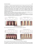
four principles are interpreted differently in different cultures. In figure 1 the four basic
principles of the common morality are presented.


Fig. 1. The four basic principles of the common morality. A brief formulation of the four
ethical principles: respect for autonomy, beneficence, nonmaleficence, and justice
(Beauchamp & Childress, 2009; Ebbesen, 2009).
Respect for autonomy
• “As a negative obligation: Autonomous actions should not be subjected to controlling
constraints by others” (Beauchamp & Childress, 2009, p. 104).
• “As a positive obligation, this principle requires both respectful treatment in disclosing
information and actions that foster autonomous decision making” (Beauchamp & Childress,
2009, p. 104). Furthermore, this principle obligates to “disclose information, to probe for and
ensure understanding and voluntariness, and to foster adequate decision making”
(Beauchamp & Childress, 2009, p. 104).
The Principle of Beneficence
• One ought to prevent and remove evil or harm
• One ought to do and promote good (Beauchamp & Childress, 2009, p. 151).
The Principle of Nonmaleficence
• “One ought not to inflict evil or harm”, where harm is understood as “thwarting, defeating, or
setting back some party’s interests” (Beauchamp & Childress, 2009, pp. 151-152).
The Principle of justice
Beauchamp & Childress do not think that a single principle can address all problems of distributive
justice (Beauchamp & Childress, 2009, p. 241). They defend a framework for allocation that
incorporates both utilitarian and egalitarian standards. A fair health care system includes two
strategies for health care allocation: 1) a utilitarian approach stressing maximal benefit to patients
and society, and 2) an egalitarian strategy emphasising the equal worth of persons and fair
opportunity (Beauchamp & Childress, 2009, pp. 275, 281).

Advanced Biomedical Engineering

210
4. Managing complex cases of biomedicine
The four ethical principles of respect for autonomy, beneficence, nonmaleficence, and justice
can be used when managing complex or problematic cases of biomedicine. When the
principles are used in biomedicine it is often necessary to make the principles specific for
that actual case. A specification of a principle is to narrow its scope and making it action-
guiding. Beauchamp & Childress explain specification as “a process of reducing the
indeterminate character of abstract norms and generating more specific, action-guiding
content” (Beauchamp & Childress, 2009, p. 17). Specification involves a fine-tuning of the
range and scope of the principle by increasing information about that specific situation
(what time, where, what persons are involved, and so forth). Each principle is prima facie
binding, which means that it “must be fulfilled unless it conflicts, on a particular occasion,
with an equal or stronger obligation” (Beauchamp & Childress, 2009, p.15). If principles
conflict they can be justifiably overridden which is the act of balancing (meaning that none
of the principles are absolute). Balancing principles tells about their weight and strength,
when balancing two principles, one principle is infringed by another (Beauchamp &
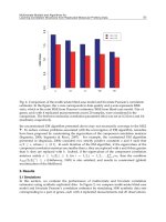
Childress, 2009, pp. 19-20). Beauchamp & Childress list six conditions that must be met to
justify the infringement of one prima facie principle by another (figure 2). Beauchamp &
Childress state that physicians’ acts of balancing and specifying ethical principles often
involve “sympathetic insight, humane responsiveness, and the practical wisdom of
evaluating a particular patient’s circumstance and needs” (Beauchamp & Childress,
2009, p. 22).


Fig. 2. Conditions constraining balancing. Conditions that must be met to justify
infringement of one prima facie norm in order to adhere to another (Beauchamp &
Childress, 2009; Ebbesen, 2009).
5. Empirical justification of the common morality

The Danish physician and philosopher Soeren Holm states that the four principles of
Beauchamp & Childress are developed from American common morality and that they
reflect certain aspects of American society and therefore they are limited to America and
unsuited for Europe (Holm, 1997). Two Danish ethicists Jacob Rendtorff and Peter Kemp
present a European alternative to Beauchamp & Childress’ principles. Rendtorff & Kemp
state that there are four ethical principles specifically suited for managing problematic cases
of biomedicine in Europe, namely the principles of autonomy, dignity, integrity, and

1. “Good reasons can be offered to act on the overriding norm rather than on the infringed
norm”.
2. “The moral objective justifying the infringement has a realistic prospect of achievement”.
3. “No morally preferable alternative actions are available”.
4. “The lowest level of infringement, commensurate with achieving the primary goal of the
action, has been selected”.
5. “Any negative effects of the infringement have been minimized”
6. “All affected parties have been treated impartially” (Beauchamp & Childress, 2009, p. 23).