Advanced Biomedical Engineering Part 2 docx

Spatial Unmasking of Speech Based on Near-Field Distance Cues

11
3.3 Discussion
For a target and masker talker located at a fixed azimuth, target identification improved
when the target was moved increasingly nearer to the head (relative to the case where both
talkers were co-located at 1 m), but got worse when the masker moved closer. This basic
pattern of results was likely driven by energetic effects: the closer source dominates the
mixture and this either increases or reduces the effective TMR at the better ear depending on
which source is moved.
The remaining benefit of spatial separation after the TMR changes were accounted for was
restricted to a better-ear TMR region around 0 dB. This region is approximately where the
psychometric function for the co-located case shows a clear plateau, which is no longer
present in the separated cases. This plateau has been described previously (Egan et al., 1954;
Dirks and Bower, 1969; Brungart et al., 2001), and is thought to represent the fact that
listeners have the most difficulty segregating two co-located talkers when they are equal in
level (0-dB TMR), but with differences in level listeners can attend to either the quieter or
the louder talker. Apparently the perception of separation in distance also alleviates the
particular difficulty of equal-level talkers, by providing a dimension along which to focus
attention selectively. This finding adds to a growing body of evidence indicating that spatial
differences can aid perceptual grouping and selective attention. Interestingly, the effect does
not appear to be “all or nothing”; larger separations in distance gave rise to larger
perceptual benefits. The lack of a spatial benefit at other TMRs, especially at highly negative
TMRs, suggests that the main problem was audibility and not confusion between the target
and the masker. Consistent with this idea, in the co-located condition, masker errors made
up a larger proportion of the total errors as the TMR approached 0 dB. In Experiment 1, the
proportion of masker errors was 38%, 45%, 62%, and 93% at -30, -20, -10, and 0-dB TMR.
Listeners in Experiment 1 performed around 10-20 percentage points better than Brungart
and Simpson’s (2002) listeners for the same stimulus configurations. This may be simply due
to differences in the cohort of listeners, but there are two methodological factors that may

have also played a role. Firstly, their study used HRTFs measured from an acoustic
mannequin as opposed to individualized filters and thus the spatial percept may have been
less realistic and thus less perceptually potent. Secondly, while the two studies used the
same type of stimuli, Brungart and Simpson used a low-pass filtered version (upper cut-off
of 8 kHz) and we used a broadband version (upper cut-off of 16 kHz). Despite the difference
in overall scores, the mean benefit (in percentage points) obtained by separating talkers in
distance was equivalent across the two studies.
4. Experiment 2
4.1 Experimental conditions
Experiment 2 was identical to Experiment 1 and used the same set of spatial configurations
and TMRs (Fig. 2 and Table 1). The only difference was that the stimuli were all low-pass
filtered (before RMS level equalization) at 2 kHz using an equiripple FIR filter with a
stopband at 2.5 kHz that is 50 dB down from the passband.
4.2 Results
4.2.1 Masker fixed at 1 m and target near
The left column of Fig. 4 shows results from the conditions in which the masker was fixed at
1 m and the target was moved into the near field for the low-pass filtered stimuli of

Advanced Biomedical Engineering

12
Experiment 2. The raw data followed a similar trend to that observed in Experiment 1 (Fig.
4, top left). As the target was moved closer to the listener, performance improved, with best
performance in the 0.12-m target case. A two-way repeated-measures ANOVA on the
arcsine-transformed data revealed that there was a significant effect of target distance
(F
2,14
=332.9, p<.01) and TMR (F
3,21
=120.6, p<.01) and a significant interaction (F

6,42
=5.1,
p<.05).
When the psychometric functions were plotted as a function of better-ear TMR, the results
for all three distances were very similar (Fig. 4, middle left). After taking into account level
changes with distance, there appears to be only a minor additional perceptual benefit of
separating the low-pass filtered target and masker in distance. Fig. 4 (bottom left) shows
that the advantage of separating the target from the masker was positive only for the small
TMR range between -5 and +5 dB. The advantages across TMR were also smaller than those
observed in Experiment 1. However, the advantages were still significant for both the 0.25-
m target (mean 13 percentage points, t
7
=4.20, p<.01) and the 0.12-m target (mean 17
percentage points, t
7
=4.88, p<.01).
A three-way ANOVA with factors of bandwidth, distance, and TMR was conducted
to compare performance in Experiments 1 and 2 in the target-near configuration
(compare Fig. 3 and Fig. 4, top left). The main effect of bandwidth was significant
(F
1,7
=8.9, p<.05), indicating that performance was poorer for low-passed stimuli than
for broadband stimuli overall. A separate two-way ANOVA on the benefits at 0 dB
(compare Fig. 3 and Fig. 4, bottom left) found a significant main effect of distance
(F
1,7
=14.5, p<.01) but no significant effect of bandwidth (F
1,7
=3.7, p=.10) and no interaction
(F

1,7
=0.7, p=.44).
4.2.2 Target fixed at 1 m and masker near
For the opposite configuration, where the masker was moved in closer (Fig. 4, right column),
results were similar to those in Experiment 1. Listeners were less accurate at identifying
the target when the masker was moved closer (Fig. 4, top right). A two-way repeated-
measures ANOVA on the arcsine-transformed data revealed a significant effect of target
distance (F
2,14
=76.4, p<.01) and TMR (F
3,21
=260.2, p<.01) and a significant interaction
(F
6,42
=5.1, p<.01).
Normalization of the curves based on better-ear TMR (Fig. 4, middle right) resulted in a
reversal of the result, showing that there was indeed a perceptual benefit once the
energetic disadvantage of a near masker was accounted for. Normalized scores
were higher for maskers at 0.12 m and 0.25 m relative to 1 m, particularly around 0-dB
TMR. This is reinforced by the benefit plots (Fig. 4, bottom right) which show that there
was a positive advantage across all TMRs. Again, the largest advantage was observed at
0-dB TMR and was statistically significant for both the 0.25-m masker (mean 24
percentage points, t
7
=7.31, p<.01) and the 0.12-m masker (mean 32 percentage points,
t
7
=7.51, p<.01).
A three-way ANOVA comparing the results from Experiments 1 and 2 in the masker-near
configuration (compare Fig. 3 and Fig. 4, top right) revealed that performance was poorer

for low-passed stimuli than for broadband stimuli overall (F
1,7
=11.7, p<.05). A two-way
ANOVA conducted on the benefits at 0 dB (compare Fig. 3 and Fig. 4, bottom right) found a
significant main effect of distance (F
1,7
=11.1, p<.05), but no significant effect of bandwidth
(F
1,7
=0.2, p=.66) and no interaction (F
1,7
=0.6, p=.47).

Spatial Unmasking of Speech Based on Near-Field Distance Cues

13

Fig. 4. Mean performance data averaged across all 8 subjects (error bars show standard
errors of the means) in Experiment 2. The left panel displays the raw (top) and normalized
(middle) data for the conditions where the masker was fixed at 1 m and the target was
moved closer to the listener. The right panel displays the raw (top) and normalized (middle)
data for the conditions where the target was fixed at 1 m and the masker was moved in
closer to the listener. The bottom panels display the benefits of separation in distance,
expressed as a difference in percentage points relative to the co-located case.

Advanced Biomedical Engineering

14
4.3 Discussion
The results from Experiment 2 in which the speech stimuli were low-pass filtered at 2 kHz

were largely similar to those from Experiment 1. Performance across conditions was
generally poorer, consistent with a more difficult segregation task, and subjects reported
that voices appeared muffled and were more difficult to distinguish from each other in this
condition. However, the perceptual benefit of separating talkers in distance condition was
for broadband and low-pass filtered stimuli. This demonstrates that the low-frequency ILDs
that are unique to this near field region of space are sufficient to provide a benefit for speech
segregation.
5. Experiment 3
5.1 Experimental conditions
In Experiment 3, three talkers were used, and they were separated in azimuth at -50°, 0°,
and 50° as illustrated in Fig. 5. For a given block, the distance of all talkers was set to either 1
m, 0.25 m or 0.12 m from the listener’s head. Six different TMR values were tested for each
spatial configuration (see Table 2), resulting in 18 unique conditions. The location of the
target within the three-talker array was varied randomly within each block, such that half
the trials had the target in the central position and the other half had the target in one of the
side positions. Two 40-trial blocks were completed per condition by each listener resulting
in a total of 2x40x18=1440 trials per listener. The distance and TMR were kept constant
within a block, but the order of blocks was randomized.


Fig. 5. The spatial configurations used in Experiment 3. Three talkers were spatially
separated in azimuth at -50°, 0° and 50°and were either all located at 1 m, 0.25 m or 0.12 m
from the listener’s head. The location of the target talker was randomly varied (left, middle,
right).

Spatial Unmasking of Speech Based on Near-Field Distance Cues

15

Configuration

(target position/distance of mixture)
TMRs tested (dB) Normalization shift (dB)
Central target 1 m [-20 -15 -10 -5 0 5] -3
0.25 m [-20 -15 -10 -5 0 5] -5
0.12 m [-20 -15 -10 -5 0 5] -8
Lateral target 1 m [-20 -15 -10 -5 0 5] 0
0.25 m [-20 -15 -10 -5 0 5] +3
0.12 m [-20 -15 -10 -5 0 5] +6
Table 2. The range of TMR values tested and normalization values for each spatial
configuration in Experiment 3. The normalization shifts are the differences in TMR at the
better ear that resulted from variations in distance and configuration.
5.2 Results
5.2.1 Centrally positioned target
When the target was directly in front of the listener, with a masker on either side at ±50°
azimuth, moving the whole mixture closer to the head had very little effect on raw
performance scores (Fig. 6, top left). A two-way repeated-measures ANOVA on the arcsine-
transformed data, however, showed that the effect of distance was statistically significant
(F
2,14
=7.7, p<.01), as was as the effect of TMR (F
5,35
=159.4, p<.01). The interaction did not
reach significance (F
10,70
=1.4, p=0.2).
When the psychometric functions were re-plotted as a function of better-ear TMR, the
distance effects were more pronounced (Fig. 6, middle left). This normalization compensates
for the fact that the lateral maskers increase more in level than the central target when the
mixture approaches the head. Mean performance was better for most TMRs when the
mixture was moved into the near field. Fig. 6 (bottom left) shows the difference (in

percentage points) between the near field conditions and the 1-m case, illustrating the
advantage of moving sources closer to the head. The mean benefits were significant at all
TMRs for both distances (p<.05).
5.2.2 Laterally positioned target
Raw results for the condition in which the target was located to the side of the three-talker
mixture are shown in Fig. 6 (top right). Performance was better when the mixture was closer
to the listener (0.12 m>0.25 m>1 m) particularly for low TMRs (below -5 dB). At higher
TMRs, performance for all three distances appears to converge. Performance generally
increased with increasing TMR but reached a plateau at around 80%. A two-way repeated-
measures ANOVA on the arcsine-transformed data confirmed that there was a main effect
of both distance (F
2,14
=24.5, p<.01) and TMR (F
5,35
=104.4, p<.01) and a significant interaction
(F
10,70
=17.4, p<.01).
When the psychometric functions were normalized to account for level changes at the better
ear, the distinction between the different distances was reduced. An advantage of the near
field mixtures over the 1-m mixture was found only at low TMRs (Fig. 6, middle right).

Advanced Biomedical Engineering

16

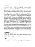
Fig. 6. Mean performance data averaged across all 8 subjects (error bars show standard
errors of the means) in Experiment 3. The left panel displays the raw (top) and normalized
(middle) data for the conditions where the target was located in the middle of three talkers.
The right panel displays the raw (top) and normalized (middle) data for the conditions

where the target was located to one side. The bottom panels display the benefits of
decreasing the distance of the mixture, expressed as a difference in percentage points
relative to the 1-m case.

Spatial Unmasking of Speech Based on Near-Field Distance Cues

17
At higher TMRs, the curves in fact reversed in order. These effects are reiterated in the
benefit plots (Fig. 6, bottom right). The advantage was positive at negative TMRs but
negative at positive TMRs. The mean benefits were significant at -15-dB TMR (t
7
=4.30,
p<.01) for the 0.25-m condition and at -10-dB TMR (t
7
=2.78, p<.05) for the 0.12-m condition.
A significant disadvantage was observed at 5-dB TMR for both distances (p<.05).
5.3 Discussion
Experiment 3 investigated the effect of moving a mixture of three talkers (separated in
azimuth) closer to the head. Given that this manipulation essentially exaggerates the
spatial differences between the competing sources, we were interested in whether it might
improve segregation of the mixture. The manipulation had different effects depending on
the location of the target. When the target was located in the middle, raw performance
improved only very slightly with distance. However, this improvement occurred despite
a decrease in TMR at the ear (both ears are equivalent given the symmetry) in this
configuration (Table 2). In other words, performance improved despite an energetic
disadvantage when the mixture was moved closer. Normalized performance thus
revealed a perceptual benefit. When the target was located to the side, moving the
mixture closer provided increases in better-ear TMR, and raw performance reflected this,
but even after normalization there was a perceptual benefit of moving the mixture in
closer. We attribute these benefits to an exaggeration of the spatial cues for the sources to

the side, giving rise to a greater perceptual distance between the sources. It is not clear to
us why this benefit was biased towards the lower TMRs in both cases, although the
drop in benefit for high TMRs appears to be related to the flattening of the psychometric
functions at high TMRs at the near field distances. It is possible that performance
reaches a limit here due to the distracting effect of having three loud sources close to the
head.
6. Conclusions
The results from these experiments provide insights into how the increase in ILDs that
occurs in the auditory near field can influence the segregation of mixtures of speech. Spatial
separation of competing sources in distance, as well as reducing the distance of an entire
mixture of sources, led to improvements in terms of the intelligibility of a target source.
These improvements were in some cases partly explained by changes in level that increased
audibility, but in other cases occurred despite decreases in target audibility. The remaining
benefits were attributed to salient spatial cues that aided perceptual streaming and lead to a
release from informational masking.
In terms of binaural hearing-aids with the capability of exchanging audio signals, the
experimental findings described here with normally-hearing listeners indicate that there
may be value in investigating binaural signal processing algorithms that apply near-field
sound transformations to sounds that are clearly lateralized. In other words, when the ITD
or ILD cues strongly indicate a lateralized sound is present, a near-field sound
transformation can be applied which artificially brings the sound perceptually closer to the
head. We anticipate further experiments conducted with hearing-impaired listeners to
investigate the value of such a binaural hearing-aid algorithm.

Advanced Biomedical Engineering

18
7. References
Arbogast, T. L., Mason, C. R., and Kidd, G. (2002). The effect of spatial separation on
informational and energetic masking of speech. Journal of the Acoustical Society of

America, Vol. 112, pp. 2086-2098.
Bolia, R. S., Nelson, W. T., Ericson, M. A., and Simpson, B. D. (2000). A speech corpus for
multitalker communications research. Journal of the Acoustical Society of America,
Vol. 107, pp. 1065-1066.
Bronkhorst, A. W. (2000). The cocktail party phenomenon: A review of research on
speech intelligibility in multiple-talker conditions. Acustica, Vol. 86, pp. 117-
128.
Bronkhorst, A. W., and Plomp, R. (1988). The effect of head-induced interaural time and
level differences on speech intelligibility in noise. Journal of the Acoustical Society of
America, Vol. 83, pp. 1508-1516.
Brungart, D. S. (1999). Auditory localization of nearby sources. III. Stimulus effects. Journal
of the Acoustical Society of America, Vol. 106, pp. 3589-3602.
Brungart, D. S., Durlach, N. I., and Rabinowitz, W. M. (1999). Auditory localization of
nearby sources. II. Localization of a broadband source. Journal of the Acoustical
Society of America, Vol. 106, pp. 1956-1968.
Brungart, D. S., and Rabinowitz, W. R. (1999). Auditory localization of nearby sources.
Head-related transfer functions. Journal of the Acoustical Society of America, Vol. 106,
pp. 1465-1479.
Brungart, D. S., and Simpson, B. D. (2002). The effects of spatial separation in distance on the
informational and energetic masking of a nearby speech signal. Journal of the
Acoustical Society of America, Vol. 112, pp. 664-676.
Brungart, D. S., Simpson, B. D., Ericson, M. A., and Scott, K. R. (2001). Informational and
energetic masking effects in the perception of multiple simultaneous talkers. Journal
of the Acoustical Society of America, Vol. 110, pp. 2527-2538.
Byrne, D. (1980). Binaural hearing aid fitting: research findings and clinical application, In
Binaural Hearing and Amplification: Vol 2, E.R. Libby, pp. 1-21, Zenetron Inc.,
Chicago, IL
Byrne, D., Nobel, W., Lepage, B. W., (1992). Effects of long-term bilateral and unilateral
fitting of different hearing aid types on the ability to locate sounds. J. Am. Acad.
Audiology, Vol. 3, pp. 369-382.

Dirks, D. D., and Bower, D. R. (1969). Masking effects of speech competing messages. Journal
of Speech and Hearing Research, Vol. 12, pp. 229-245.
Drennan, W. R., Gatehouse, S. G., and Lever, C. (2003). Perceptual segregation of competing
speech sounds: The role of spatial location. Journal of the Acoustical Society of
America, Vol. 114, pp. 2178-2189.
Duda, R. O., and Martens, W. L. (1998). Range dependence of the response of a
spherical head model. Journal of the Acoustical Society of America, Vol. 104, pp.
3048-3058.
Durlach, N. I., and Colburn, H. S. (1978). Binaural phenomena, In The Handbook of Perception,
E. C. Carterette and M. P. Friedman, Academic, New York.

Spatial Unmasking of Speech Based on Near-Field Distance Cues

19
Durlach, N. I., Thompson, C. L., and Colburn, H.A. (1981). Binaural interaction in impaired
listeners - a review of past research. Audiology, Vol. 20, pp. 181-211.
Ebata, M. (2003). Spatial unmasking and attention related to the cocktail party problem.
Acoust. Sci and Tech. , Vol. 24, pp. 208-219.
Egan, J., Carterette, E., and Thwing, E. (1954). Factors affecting multichannel listening.
Journal of the Acoustical Society of America, Vol. 26, pp. 774-782.
Feuerstein, J. (1992). Monaural versus binaural hearing: ease of listening, word recognition,
and attentional effort. Ear and Hearing, Vol. 13,, No. 2, pp. 80-86.
Freyman, R. L., Helfer, K. S., McCall, D. D., and Clifton, R. K. (1999). The role of perceived
spatial separation in the unmasking of speech. Journal of the Acoustical Society of
America, Vol. 106, pp. 3578-3588.
Hirsh, I. J. (1950). The relation between localization and intelligibility. Journal of the Acoustical
Society of America, Vol. 22, pp. 196-200.
Kan, A., Jin, C., and van Schaik, A. (2009). A psychophysical evaluation of near-field head-
related transfer functions synthesized using a distance variation function. Journal of
the Acoustical Society of America, Vol. 125, pp. 2233-2243.

Kidd, G., Jr., Mason, C. R., Richards, V. M., Gallun, F. J., and Durlach, N. I. (2008).
Informational masking, In Auditory Perception of Sound Sources, W. A. Yost, A. N.
Popper, and R. R. Fay (Springer Handbook of Auditory Research, New York), pp.
143-190.
Kidd, G., Jr., Mason, C. R., Rohtla, T. L., and Deliwala, P. S. (1998). Release from
masking due to spatial separation of sources in the identification of nonspeech
auditory patterns. Journal of the Acoustical Society of America, Vol. 104, pp. 422-
431.
Libby, E. R. (2007). The search for the binaural advantage revisited. The Hearing Review,
Vol. 14, No. 12, pp. 22-31.
Moore, B.C.J. (2007). Binaural sharing of audio signals: Prospective benefits and limitations.
The Hearing Journal, Vol. 40, No. 11, pp. 46-48.
Pralong, D., and Carlile, S. (1994). Measuring the human head-related transfer
functions: A novel method for the construction and calibration of a miniature
"in-ear" recording system. Journal of the Acoustical Society of America, Vol. 95, pp.
3435-3444.
Pralong, D., and Carlile, S. (1996). The role of individualized headphone calibration for the
generation of high fidelity virtual auditory space. Journal of the Acoustical Society of
America, Vol. 100, pp. 3785-3793.
Rabinowitz, W. M., Maxwell, J., Shao, Y., and Wei, M. (1993). "Sound localization cues for a
magnified head: Implications from sound diffraction about a rigid sphere,"
Presence: Teleoperators and Virtual Environments 2.
Shinn-Cunningham, B. G., Schickler, J., Kopco, N., and Litovsky, R. (2001). "Spatial
unmasking of nearby speech sources in a simulated anechoic environment. Journal
of the Acoustical Society of America, Vol. 110, pp. 1119-1129.
Studebaker, G. A. (1985). A rationalized arcsine transform. Journal of Speech and Hearing
Research, Vol. 28, pp. 455-462.

Advanced Biomedical Engineering

20
Zurek, P. M. (1993). Binaural advantages and directional effects in speech intelligibility, In
Acoustical Factors Affecting Hearing Aid Performance, G. A. Studebaker and I.
Hochberg, pp. 255-276, Allyn and Bacon, Boston.
2
Pulse Wave Analysis
Zhaopeng Fan, Gong Zhang and Simon Liao
University of Winnipeg
Canada
1. Introduction
Cardiovascular refers to the Cardio (heart) and vascular (blood vessels). The system has two
major functional parts: central circulation system and systemic circulation system. Central
circulation includes the pulmonary circulation and the heart from where the pulse wave is
generated. Systemic circulation is the path that the blood goes from and to the heart. (Green
1984) Pulse wave is detected at arteries which include elastic arteries, medium muscular
arteries, small arteries and arterioles. The typical muscular artery has three layers: tunica
intima as inner layer, tunica media as middle layer, and tunica adventitia for the outer layer.
(Kangasniemi & Opas 1997) The material properties of arteries are highly nonlinear.
(langewouters et al. 1984) It depends on the contents of arterial wall: how collagen, elastin
and protein are located in the arteries. Functional and structural changes in the arterial wall
can be used as early marker for the hypertensive and cardiac diseases.
Blood flow is the key to monitor the cardiovascular health condition since it is generated
and restrict within such system. Currently the most widely used method for haemodynamic
parameters detecting is invasive thermo-dilution method. Impedance-cardiography is the
most commonly used non-invasive method nowadays; however, it is too complex for
clinical routine check. Pulse wave analysis is an innovative method in the market to do fast
and no burden testing (Zhang et al. 2008)
Pulse is one of the most critical signals of human life. It comes directly from heart to the
blood vessel system. As pulse transmitted, reflections will occur at different level of blood
vessels. Other conditions such as resistance of blood flow, elastic of vessel wall, and blood

viscosity have clear influence on pulse. Pathological changes affect pulse in different ways:
the strength, reflection, and frequency. So pulse provides abundant and reliable information
about cardiovascular system.
Pulse can be recorded to a set of time series data and represented as a diagraph which is
called pulse waveform or pulse wave for short.
Gathering pulse at wrist by finger has been a major diagnosis method in China since 500 BC.
Physicians used palpation of the pulse as a diagnostic tool during the examination. In
300AD, “Maijing” categoried pulse into 24 types and became the first systematic literature
about the pulse. Grecian started to notice the rhythm, strength, and velocity at 400BC.
Struthius described a method to watch the pulse wave by putting a leaf on the artery, which
is considered as early stage of pulse wave monitoring. In 1860, Etienne Jules Mary invented
a level based sphygmograph to measure the pulse rate. It is the first device can actually
record the pulse wave. Frederick observed normal radial pressure wave and the carotid

Advanced Biomedical Engineering
22
wave to find the normal waveform and the differences between those waveforms.
(Mahomed 1872) He figured out the special effect on the radial waveform caused by the
high blood pressure. It helps to learn the natural history of essential
hypertension.(Mahomed 1877) The effects of arterial degeneration by aging on the pulse
wave were also shown on his work.(Mahomed 1874) His researches have been used in the
life insurance field. (Postel_Vinay 1996)
The analysis was based on the basic mathematic algorithms in nineteenth century:
dividing the wave into increasing part and decreasing part, calculating the height and
area of the wave. Calculus, hemodynamic, biomathematics and pattern recognition
techniques has been used in pulse wave analysis by taking advantage of Information
Technology. However, utilizing the classic pulse theory with current techniques is still a
big challenge.
2. Pulse wave analysis methods
2.1 Research data source

With informed consent, 517 sets of testing data were collected from 318 subjects. The ages of
subjects range from 1 to 91 years (mean ± SD, 55 ± 20). 87 subjects were chosen from normal
people (mean ±SD, 51 ±17) and the rest were recorded from patients in Department of
Cardiology at Shandong Provincial Hospital in China (mean ± SD, 62 ±13). Normal people
were assigned to the control group corresponding to the patients group. All medical records
were collected in order to do research on each risk factor. Risk factor groups, including
smoking group (mean ±SD, 66.089±13.112) and diabetes group (mean ±SD, 64±11.941), are
created based on the risk factors from medical records.
2.2 Pulse wave factors
Using pulse data directly is unreliable since any change of haemodynamic condition has
effects on pulse wave data. But there are still many researches for pulse wave analysis
because the pulse data is much easier and safer to get than most other signals. With
considering related conditions, pulse wave factors analysis can achieve higher accuracy.
Most recent researches give positive results with comparing pulse wave factors analysis and
standard methods. Pathophysiological Laboratory Netherlands did study on continuous
cardiac output monitoring with pulse contour during cardiac surgery (Jansen 1990). Cardiac
output was measured 8 to 12 times during the operation with pulse contour and
thermodilution. The result shows linear regression between two methods. The cardiac
output calculated by pulse wave factors is accurate even when heart rate, blood pressure,
and total peripheral resistance change.
To reduce the effects of other factors, pulse wave factors had been tested among different
groups. Rodig picked two groups of patients based on ejection fraction: 13 patients in group
1 with ejection fraction greater than 45% and 13 patients in group 2 with ejection fraction
less than 45%. Both pulse wave factors and thermodilution technique had been used to
calculate the cardiac output 12 times during the surgery. The mean differences for CO did
not differ in either group (Rodig 1999). The differences became significant when systemic
vascular resistance increased by 60% and early period after operation. It suggested that
pulse wave factors analysis is a comparable method during the surgery. Calibration of the
device will help to achieve more accurate result.

Pulse Wave Analysis
23
The patients with weak pulse waveform or arrhythmia should always avoid using the
result of pulse wave factors as the major source since it become unreliable in such
environment.
Early Detection of cardiovascular diseases is one of the most important usages for pulse
wave monitoring. The convenience noninvasive technique makes it extremely suitable for
widely use at community levels. Factors derived from pulse wave analysis have been used
to detect hypertension, coronary artery diseases. For example, losing the diastolic
component is the result of reduced compliance of arteries. (Cohn 1995) Pulse wave is
suggested to be early marker for those diseases and guide for health care professions during
the therapy.
Pulse wave were used to be analyzed in two ways: point based analysis, area based analysis.
Point based analysis is usually designed for specific risk factor. It picks up top, bottom
points from different components of the waveform or derivative curve. Then the calculation
is done regarding to the medical significant of those points. Stiffness Index is a well-known
factor in this category.
Arteries stiffen is a consequence of age and atherosclerosis. Two of the leading causes of
death in the developed world in nowadays, myocardial infarction and stroke, are a direct
consequence of atherosclerosis. Arterial stiffness is an indicator of increased cardiovascular
disease risk. Among many new methods applied to detect arterial stiffness, pulse wave
monitoring is a rapidly developing one.
Arterial pulse is one of the most fundamental life signals in medicine, which has been used
since ancient time. With the help of new information technology, pulse wave analysis has
been utilized to detect many aspects of heart diseases especially the ones involving arterial
stiffness.
Total arterial compliance and increased central Pulse Wave Velocity (PWV) are associated
with arterial wall stiffening. They are recognized as the dominant risk factors for
cardiovascular disease. The contour of the peripheral pressure and volume pulse affected
by the vascular aging on the upper limb is also well-known. The worsen artery stiffness

with an increase in pulse wave velocity is cited as the main reason for the change of pulse
contour.
PWV is the velocity of the pulse pressure. The blood has speed of several meters per second
at the aorta and slow down to several mm per second at peripheral network. The PWV is
much faster than that. Normal PWV has the range from 5 meters per second to 15 meters per
second. (O’Rourke & Mancia 1999)
Since pulse pressure and pulse wave velocity are closely linked to cardiovascular morbidity,
some non- invasive methods to assess arterial stiffness based on pulse wave analysis have
been introduced. However, these methods need to measure the difference of centre artery
pulse and the reflected pulse wave, which is a complicated process. On the other hand, the
Digital Volume Pulse (DVP) may be obtained simply by measuring the blood volume of
finger, which becomes a potentially attractive waveform to analyze.
Millasseau et al have demonstrated that arterial stiffness, as measured by peripheral pulse
wave analysis, is correlated with the measurement of central aortic stiffness and PWV
between carotid and femoral artery, which is considered as a reliable method in assessment
of cardiovascular pathologic changes for adults. They introduced the Stiffness Index (SI),
which was derived from the pulse wave analysis for artery stiffness assessment and was

Advanced Biomedical Engineering
24
correlated with PWV (r=0.65, P<0.0001). It is an effective non-invasive method for assessing
artery stiffness.
Pulse Wave Velocity is the golden standard for arterial stiffness diagnosis. Researches show
that Stiffness Index has equivalent output as PWV. It uses the reflection of the pulse as the
second source to get the time difference without additional sensors which make it more
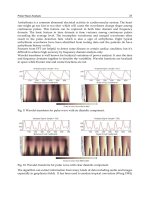
applicable to the Home Monitoring System. As shown in figure 1, the systolic top shows the
time that pulse reach the finger; diastolic top represents the time that pulse reflection reach
the finger. The distance that pulse goes through has direct relationship with the height of the
subject. SI can be calculated by h/Δt.
Area Based analysis specialized in the blood volume monitoring such as Cardiac Output

(CO). The attempt for getting cardiac output from pulse wave started more than one
hundred years ago (Erlanger 1904). The pulse wave is the result of interaction between
stroke volume and arteries resistance. Building the model of arterial tree helped the
calculation of CO from pulse wave. The simplest model used in clinic contains single
resistance. Other elements should be involved in the calculation including capacitance
element, resistance element (Cholley 1995).
Not all models have reliable results, even some widely used one can only work in specific
environment. Windkessel Model consists of four elements: left ventricle, aortic valve,
arterial vascular compartment, and peripheral flow pathway. Testing of the model in
normotensive and hypertensive subjects shows that the model is only valid when the
pressure wave speed is high enough with no reflection sites exist (Timothy 2002).
Cardiac Index (CI) is an important parameter related to the CO and body surface area.
Tomas compared the CI value among pulmonary artery thermodilution, arterial
thermodilution and pulse wave analysis for critically ill patients. The mean differences
among three methods are within 1.01% and standard derivation are within 6.51%. (Felbinger
2004) The pulse wave factors provide clinically acceptable accuracy.
In addition to long term monitoring, pulse wave analysis is also useful for emergency
environment. Cardiac Function can be evaluated within several seconds.
2.1.1 Stiffness Index
The pulse wave sensor detects the blood flow at the index finger and tracks the strength of
the flow as pulse wave data. To record the pulse wave, the patients were comfortably rested
with the right hand supported. A pulse wave sensor was applied to the index finger of right
hand. Only the appropriate and stable contour of the pulse wave was recorded.
As shown in Figure, the first part of the waveform (systolic component) is result of pressure
transmissions along a direct path from the aortic root to the wrist. The second part (diastolic
component) is caused by the pressure transmitted from the ventricle along the aorta to the
lower body. The time interval between the diastolic component and the systolic component
depends upon the PWV of the pressure waves within the aorta and large arteries which is
related to artery stiffness. The SI is an estimate of the PWV about artery stiffness and is
obtained from subject height (h) divided by the time between the systolic and diastolic

peaks of the pulse wave contour. The height of the diastolic component of the pulse wave
relates to the amount of pressure wave reflection.
SI is highly related to the pulse rate because it is calculated by the time interval between
systole and diastole. Younger people with high pulse rate can get a relative high score than
older people with slow pulse rate. Adjustment based on pulse rate can be applied on SI
calculation.

Pulse Wave Analysis
25
The testing results based on age are shown in Figure and Figure, which indicate that the
adjusted SI is more sensitive than SI.


Fig. 1. Stiffness index is related to the time delay between the systolic and diastolic
components of the waveform and the subject’s height

SI by Age
Age
0 20406080100
SI
2
4
6
8
10
12
14
16
18
20

22
Age vs SI
Plot 1 Regr
Adjusted SI by Age
Age
0 20406080100
SI for Standard Pulse Rate
2
4
6
8
10
12
14
16
18
20
22
Age vs Standard SI
Plot 1 Regr

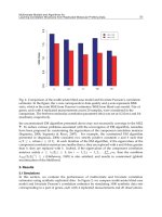
Fig. 2. Correlation for Stiffness Index and age (r=0.275, p = 9.833E-019). A closer relationship
could be found between adjusted Stiffness Index and age. (r=0.536, p=7.279E-040)
In order to test the sensitivity of primary factor SI, we compare it with the collected data
from different groups.
SI is much higher in patients group (SI: 9.576±2.250) than that of control group (SI:
7.558±1.751). On the other hand, it has positive correlation with age for both groups. All
people in patients group came from the Department of Cardiology at Shandong Provincial
Hospital and most of them have atherosclerosis which is the main reason for arterial
stiffness. This result shows that the SI is a significant factor in pulse wave analysis to detect

the degree of arterial stiffness.

Advanced Biomedical Engineering
26
Risk factor groups are very import in this research. Diabetes group (SI: 9.975±2.174) and
smoking group (SI: 10.039±2.587) have even higher SI than patients group as a whole. SI is
reliable for research to detect risk factors.
By analyzing with different factors, SI is found to be correlated with age, weight, and
systolic blood pressure. With the comparison of patients and control groups, we find that SI
has less correlation with age for patients with heart disease. However, when people have
other risk factors such as smoking and diabetes, SI has no longer visible correlation with
age. It also indicates that SI is sensitive to cardiovascular diseases and risk factors. People
who have cardiovascular diseases or risk factor will have higher than normal SI. In general,
illness and risk factors will have more impact on SI. This makes SI a perceptible indication in
diagnosing arterial stiffness.
SI can be affected by the cardiac condition as we described before. The adjusted SI can only
rectify influence of heart rate in a certain level. Other abnormal cardiac conditions, such as
heart failure, will disturb the pulse wave form in different ways. A basic judgment of
cardiac condition will make SI more catholicity.
2.1.2 Cardiac Output
The pulse contour method for calculation of cardiac output can be done based on the theory
of elastic cavity (Liu & Li, 1987).
• Blood flow continuous equation:

1
2
0
in out
out
dV

QQ
dt
dV
Q
dt
=+
+=
(1)
where
Q
in
is the volume of blood flowing into the artery and Q
out
is the volume of blood
flowing into the vein.
t
1
and t
2
are the systolic and diastolic period, respectively.
•
Equation between pressure remainder and blood flow:

v
out
p
p
Q
R
−

=
(2)
where
p is the arterial pressure, p
v
is the venous pressure, and R indicates the peripheral
resistance of cardiovascular system.
•
Arterial pressure volume equation:

dV
AC
d
p
=
(3)
where AC is a constant that depends on the arterial compliance.
Based on the above three equations, the analytic equation of elastic cavity can be calculated:

1
2
0
v
in
v
d
ppp
QAC
dt R
dp p p

AC
dt R
−
=+
−
+=
(4)
Computing the integral of Equation (4):

Pulse Wave Analysis
27

()
()
*
*
0
S
vsd
d
ds
A
SACpp
R
A
AC p p
R
=−+
−+=
(5)

where S
v
is the stroke volume during a heartbeat. We refer to Figure 4 for A
s
, A
d
, p
s
, and p
d
.
Cardiac Output is highly correlated to age, weight, and systolic blood pressure. It shows the
working status of the heart while SI shows the degree of arterial stiffness. We can also find
that many subjects in patients group have abnormal Cardiac Output (CO: 4.567±1.309). But
there is no significant correlation between SI and CO. Therefore, CO is a good complement
of SI for analyzing cardiovascular condition.
2.3 Waveform analysis
The calculation based on the points with special meanings is very sensitive in the detection
of risks. It uses simple algorithm to achieve the balance of performance and accuracy. But
it’s difficult to evaluate the overall cardiovascular condition only with several risk factors.
The pulse is produced by the cooperation of heart, blood vessel, micro circulation and other
parties. The more information included the more accurate classification we can get. This
research used some sample wave forms to represent the different categories. A wave form
belongs to a category if it’s more similar to the wave form in that category than any other
wave forms.


Fig. 3. Variation for continue waveforms. (O’Rourke 2001)
Pulse wave is relatively stable under the testing condition: subject setting in a quite
environment and keeping calm. The pulse wave analysis result is highly repeatable in this

condition. Actually the similarity of pulse waveforms doesn’t change a lot under similar
cardiovascular health condition even the heart rate and pulse strength changed, so
waveform analysis can fit in different scenarios other than specific testing environment.
There are several classification system for the pulse wave. In the paper “Characteristics of
the dicrotic notch of the arterial pulse wave in coronary heart diease”, Tomas treat the notch
as the indicator and classify pulse wave into four categories as following:
-
Class I: A distinct incisura is inscribed on the downward slop of the pulse wave
-
Class II: No incisura develops but the line of descent becomes horizontal
-
Class III: No notch is present but a well-defined change in the angle of descent is
observed
-
Class IV: No evidence of a notch is seen

Advanced Biomedical Engineering
28


Fig. 4. Four classes of waveform based on dicrotic notch
This classification focus on the notch of the wave form which is considered as the indicator
of arterial stiffness. Bates evaluates continues wave forms to include other possible diseases.
He gave detail description of the pulse wave and discussed the cause of each pulse wave
type. Possible diseases were also provided in his research.

Pulse type Physiological cause Possible disease
small & weak
decreased stroke volume
heart failure, hypovolemia,

severe aortic stenosis
increased peripheral resistance
large & bounding
increased stroke volume fever, anaemia,
hyperthyroidism, aortic
regurgitation, bradycardia,
heart block, atherosclerosis
decreased peripheral resistance
decreased compliance
bisferiens
increased arterial pulse with double
systolic peak
aortic re
g
ur
g
itation, aortic
stenosis and regurgitation,
hypertropic
cardiomyopathy
pulsus alternans
pulse amplitude varies from peak to
peak, rhythm basically regular
left ventricular failure
Table 1. Possible diseases which can be diagnosed based on the different types of
cardiovascular pulse shapes (Bates 1995).


Fig. 5. Pulse wave classification from Bates
Class I

Class II
Class III
Class VI

Pulse Wave Analysis
29
In order to get more precise information from the wave form, researchers take the
traditional pulse diagnosis as the reference and mapping the characters of pulse diagnosis
with the pattern of wave form. It can be used to detect certain cardiovascular risk as well as
the classification. For example, acute anterior myocardial infarction will have a sharp
systolic component and very small diastolic component which suggests poor blood supply.
2.2.1 Fourier transform and wavelet
Fourier Transform and Wavelet Transform have been used to perform the basic analysis on
the pulse waveform. Fourier transform is a basic and important transform for linear analysis
which usually transfers the signal from time domain (signal based on time) to frequency
domain (the transform depends on frequency).
The Fourier theory states that any continuous signals or time serial data can be expressed as
overlay of sine waves with different frequencies. This process can help signal analysis
because the sine wave is well understood and treated as simple function in both
mathematics and physics. Fourier transform calculates the frequency, amplitude, and phase
based on this theory. Significant features could be detected by Fourier transform from
similar time series data with big differences in frequency domain.
The Fourier transform can be treated as a special calculus formula that expresses the
qualified function into sine basis functions. The function with the lowest frequency is called
the fundamental. It has the same repetition rate of the periodic signal under evaluation. The
frequency of other functions is integer times of the fundamental frequency.
Inverse Fourier transform can be used to recover the time series signal after the analysis on
frequency domain is done.
With comparing the original waveform and transform data, some special features can be
detected in the frequency domain.

The regular waveform from a normal subject has data nearly U shape distributed in the
frequency domain. Lower frequencies and higher frequencies get bigger values and the slop
goes smoothly from negative to positive. The peak value at lower frequency side is almost
50% bigger than the peak value at higher frequency side. The data become inconspicuous
for frequencies between10 and 190 Hz. The higher values in time domain will result in the
higher value in frequency domain.


Fig. 6. Fourier Transform for a typical pulse waveform
Patients with old myocardial infarction often have obtuse systolic component and weak
diastolic component due to the abnormal cardiac function. The diastolic component has a

Advanced Biomedical Engineering
30
round top and much wider than the normal waveform. This feature will generate a local
maximum value at around 7Hz and 193Hz. This feature can be used to detect the cardiac
function diseases which cause slow change rate at pulse waveform.


Fig. 7. Typical waveform of old myocardial infarction and their Fourier Transform
In a group of 100 selected testing data (50 normal waveform and 50 typical waveforms for
old myocardial infarction), 48 testing data has local maximum at around 7Hz and 52 has
smooth U shape distribution at frequency domain. 6 normal waveforms have been classified
to old myocardia infarction by mistake and 8 typical myocardia infarction waveforms were
not detected. Some possible reasons for mistake in the test:
1.
Big wide diastolic component may cause the local maximum value in frequency domain.
2.
Slow heart rate
3.

Unstable pulse
4.
Incomplete waveforms caused by device
The shape of diastolic component is important to arterial stiffness analysis. But it’s difficult
to get the corresponding features at frequency domain because the diastolic part is relatively
small and can be easily affected by systolic part in FFT. The features for arterial stiffness can
not be derived directly from the Fourier transform.


Fig. 8. Arrhythmia cause the second pulse arrives in advanced while the first pulse
waveform is not complete yet. FFT shows that multi local maximum values appear at both
higher frequency end and lower frequency end.