Aeronautics and Astronautics Part 9 pdf

Aircraft Gas-Turbine Engine’s Control Based on the Fuel Injection Control

309
The system operates by keeping a constant pressure in chamber 10, equal to the preset value
(proportional to the spring 16 pre-compression, set by the adjuster bolt 15). The engine’s
necessary fuel flow rate
i
Q and, consequently, the engine’s speed n, are controlled by the
co-relation between the
c
p
pressure’s value and the dosage valve’s variable slot
(proportional to the lever’s angular displacement

).
An operational block diagram of the control system is presented in figure 4.


TURBO-JET
ENGINE
FUEL
INJECTION
DOSAGE
VALVE
FUEL
INJECTION
PUM P
PRESSURE
CONTROL LER
(

p
c
=const.)


n
n
y
Q
p
Q
i
p
c
p
c i
(z)
x

*
1
*
1
,, TpVH
Flight regime
THROTTLE
p
c


Fig. 4. Constant pressure chamber controller’s operational block diagram
3.2 System mathematical model
The mathematical model consists of the motion equations for each sub-system, as follows:
a.
fuel pump flow rate equation

(,)
pp
QQn
y

, (5)
b.
constant pressure chamber equation

ipA
QQQ

 , (6)
c.
fuel pump actuator equations

2
2
4
A
AdA cA
d
Qpp




, (7)


0
d
d
dd
A
As A A s
p
QQ V S yy
tt



, (8)


2
2
ddy
d
d
f
sBcAA
y
mkyySpSp
t

t

  , (9)
d.
pressure sensor equations

0
2
()
snn A
Qdzxpp


   , (10)

2
12 2
()
4
n
mc A e
d
lS
p
l
p
lk z x


, (11)

e.
dosing valve equation

Aeronautics and Astronautics

310

1
2
s
ii cCA
Qb pp





, (12)
f.
jet engine’s equation (considering its speed n as controlled parameter)



**
11
,,
i
nnQ
p
T

, (13)
where , , ,
p
iAs
QQQQ are fuel flow rates,
c
p
-pump’s chamber’s pressure,
A
p
- actuator’s A
chamber’s pressure,
CA
p
-combustor’s internal pressure,
0
p
-low pressure’s circuit’s
pressure,
dA

,
n

,
i

-flow rate co-efficient,
,
An

dd
-drossels’ diameters,
,
AB
SS
-piston’s
surfaces,
AB
SS
,
m
S
-sensor’s elastic membrane’s surface, ,
fe
kk-spring elastic constants,
0A
V -actuator’s A chamber’s volume,

-fuel’s compressibility co-efficient,

-viscous
friction co-efficient, m-actuator’s mobile ensemble’s mass,

-dosing valve’s lever’s angular
displacement (which is proportional to the throttle’s displacement), x-sensor’s lever’s
displacement, z-sensor’s spring preset, y-actuator’s rod’s displacement,
**
11
,
p

T
-engine’s
inlet’s parameters (total pressure and total temperature).
It’s obviously, the above-presented equations are non-linear and, in order to use them for
system’s studying, one has to transform them into linear equations.
Assuming the small-disturbances hypothesis, one can obtain a linear form of the model; so,
assuming that each X parameter can be expressed as

 
2
0

1! 2! !
n
XX
X
XX
n


  
, (14)
(where
0
X
is the steady state regime’s X-value and
X

-deviation or static error) and
neglecting the terms which contains


,2
r
Xr


, applying the finite differences method,
one obtains a new form of the equation system, particularly in the neighborhood of a steady
state operating regime (method described in Lungu, 2000, Stoenciu, 1986), as follows:



AAc A
Qkp p


, (15)

ii icc
Qk k
p




, (16)

sSAAs s
Qk
p

kxkz

  
, (17)

ipA
QQQ

 
, (18)

0
dd
dd
AsA AA
QQV
p
S
y
tt


    
, (19)


1
2
emc
l

kxz S
p
l

  
, (20)

2
2
dd
1
d
d
f
cA
Ae e
k
m
y
ypp
Sk kt
t







, (21)

Aircraft Gas-Turbine Engine’s Control Based on the Fuel Injection Control

311
where the above used annotations are

2
10
00
2
2
,
8
ic
A
AdA i
cA
b
p
d
kk
pp









,

00 0
0
2
2
nn A
SA
A
dx z
p
k
p
 



,


10 0 0
0
22
,
2
is c nn A
ic s
c
b
p

d
p
kk
p
   
 


. (22)
Using, also, the generic annotation
0
X
X
X

 , the above-determined mathematical model can
be transformed in a non-dimensional one. After applying the Laplace transformer, one
obtains the non-dimensional linearised mathematical model, as follows



s1 s
PA A A
y
cx cz c
k
py
kx kz
p



, (23)

cx cz zxc c
kx kz k
p
 , (24)



22
0
s2 s1
A
yy y
AC c A
kT T ykpp

, (25)

p
cc
py
A
kk
p
k
yp



, (26)

cQ c Q i
kp k Q


. (27)
For the complete control system determination, the fuel pump equation (for
p
Q
) and the jet
engine equation for
n (Stoicescu & Rotaru, 1999) must be added. One has considered that the
engine is a single-jet single-spool one and its fuel pump is spinned by its shaft; therefore, the
linearised non-dimensional mathematical model (equations 23÷27) should be completed by

pp
n
py
Qknk
y
, (28)


*
1
s1
MciHV
nkQ k p


  . (29)
For the (23)÷(29) equation system the used co-efficient expressions are



0 00
00 0
00000
,,,,,,,
ASA
c Ae
ss A
AC PA cx cz A y Ay
A AAC ccASAAcAc
kk
pSyky
kx kz V
kk kk k
pkkppkkkpSp



   



0
0
1
0

20
,, , ,
2
smc
i
yzxc
eye e AA
kS p
k
ml
Tkk
kTk klkp





  




0
0
0
00 0
,,,
p
Aic
ic c

i
p
cQ
p
QcQ c
AAC AA i i
Q
kk
kp
k
kkkkk
kk kp Q Q





. (30)

Aeronautics and Astronautics

312
Based on some practical observation, a few supplementary hypotheses could be involved
(Abraham, 1986). Thus, the fuel is a non-compressible fluid, so
0


; the inertial effects are
very small, as well as the viscous friction, so the terms containing m
and


are becoming
null. The fuel flow rate through the actuator
A
Q is very small, comparative to the
combustor’s fuel flow rate
i
Q
, so
p
i
QQ

. Consequently, the new, simplified, mathematical
model equations are:
-
for the pressure sensor:

lc z
xkp kz, (31)
where

00
0
1
0020
0
0
,
cc

m
lz
ce
pp
Sz
xl x
kk
x
p
xlk x z



 





, (32)
or, considering that the imposed, preset value of
c
p
is
0
0
0
c
z
ci

lc
p
kz
pz
k
p
z






, one obtains



lci c
xk
pp
  ; (33)
-
for the actuator:



s1
y
x
y

kx

, (34)
where



00 0
00 0
2
0
00
4
,
2
Af c f
A
yAcf
s
A
fnn dAA
Skyp ky
S
pp
k
y
Q
Q
kdxd
yy


 

 
 




 

 
,

0
00
0
0
0
2
0
0
00
4
2
s
nnA f
x
s
A

nn dAA
y
Q
dp ky
xx
y
k
x
Q
Q
dx d
yy








 




 

 
. (35)
Simplified mathematical model’s new form becomes


*
1
s1
MciHV
nkQ k
p

 
, (36)

i
pp
n
py
QQ knk
y
  , (37)



lci c
xk
pp
 
; (38)

Aircraft Gas-Turbine Engine’s Control Based on the Fuel Injection Control

313



s1
y
x
y
kx


, (39)

1
ci
pp
k
pQ
kk



. (40)
One can observe that the system operates by assuring the constant value of
c
p
, the
injection fuel flow rate being controlled through the dosage valve positioning, which
means directly by the throttle. So, the system’s relevant output is the
c

p
-pressure in
chambers 10.
For a constant flight regime, altitude and airspeed (
const., const.HV

 ), which mean that
the air pressure and temperature before the engine’s compressor are constant


**
11
const., const.pT
, the term in equation (36) containing
*
1
p
becomes null.
3.3 System transfer function
Based on the above-presented mathematical model, one has built the block diagram with
transfer functions (see figure 5) and one also has obtained a simplified expression:

 
2
s1 1 s1
rpy rpy
y
Mc
p
n

y
Mc
p
nc
pp
kk kk
kk kk
p
kk
  


 




  




 




 

s1 s1 s1

py r
y
Mcpn Mci
pp
kk
k
kk
p
kk

  
   , (41)
where
rxl
kkk .


1s
M

k
c

+
n
py
k
pn
k
i

Q
i
Q
1
p
k

+
y
+
x
x
k
1s
y

l
k

l
k
z
k
z
ci
p
_
c
p
c

n
p
c
p
+
p
k

k

_

Fig. 5. System’s block diagram with transfer functions
So, one can define two transfer functions:
a.
with respect to the dosage valve’s lever angular displacement


sH

;
b.
with respect to the preset reference pressure
ci
p
, or to the sensor’s spring’s pre-
compression z,


s

z
H .
While

angle is permanently variable during the engine’s operation, the reference
pressure’s value is established during the engine’s tests, when its setup is made and

Aeronautics and Astronautics

314
remains the same until its next repair or overhaul operation, so 0
ci
zp

 and the transfer
function


s
z
H definition has no sense. Consequently, the only system’s transfer function
remains


 

2
s1 s1
s
s1 1 s1

yMcpn
p
r
py
r
py
yM cpn y M cpn
pp
k
kk
k
H
kk kk
kk kk
kk



  
 





   





, (42)
which characteristic polynomial’s degree is 2.
3.4 System stability
One can perform a stability study, using the Routh-Hurwitz criteria, which are easier to
apply because of the characteristic polynomial’s form. So, the stability conditions are

0
yM



, (43)


11 0
rpy
cpn y M
p
kk
kk
k




 


, (44)

10
rpy
cpn
p
kk
kk
k

. (45)
The first condition (43) is obviously, always realized, because both
y

and
M

are strictly
positive quantities, being time constant of the actuator, respectively of the engine.
The (40) and (41) conditions must be discussed.
The factor 1
cpn
kk is very important, because its value is the one who gives information
about the stability of the connection between the fuel pump and the engine’s shaft
(Stoicescu&Rotaru, 1999). There are two situation involving it:
a.
1
cpn
kk  , when the connection between the fuel pump and the engine shaft is a stable
controlled object;
b.
1

cpn
kk  , when the connection fuel pump - engine shaft is an unstable object and it is
compulsory to be assisted by a controller.
If
1
cpn
kk 
, the factor
1
cpn
kk

is strictly positive, so


10
cpn y
kk



. According to their
definition formulas (see annotations (35) and (30)),
,,
rppy
kkk
are positive, so
0
rpy
p

kk
k

and
10
rpy
M
p
kk
k






, which means that both other stability requests, (44) and (45), are
accomplished, that means that the system is a stable one for any situation.

Aircraft Gas-Turbine Engine’s Control Based on the Fuel Injection Control

315
If
1
cpn
kk 
, the factor
1
cpn
kk


becomes a negative one. The inequality (44) leads to



1
1
cpn
My
rpy
p
kk
kk
k









, or

1
1
rpy
p
y

M
cpn
kk
k
kk









, (46)
which offers a criterion for the time constant choice and establishes the boundaries of the
stability area (see figure 6.a).
Meanwhile, from the inequality (45) one can obtain a condition for the sensor’s elastic
membrane surface area’s choice, with respect to the drossels’ geometry (
,
An
dd) and quality


,
nA


, springs’ elastic constants



,
ef
kk , sensor’s lever arms


12
,ll
and other stability
co-efficient

,,
cpnpy
kk k



2
00
2
10
22
1
4
nn dAA f
cpn
e
m
fpy nA
dx d ky

kk
k
l
S
kl k dp
 




. (47)
Another observation can be made, concerning the character of the stability, periodic or non-
periodic. If the characteristic equation’s discriminant is positive (real roots), than the
system’s stability is non-periodic type, otherwise (complex roots) the system’s stability is
periodic type. Consequently, the non-periodic stability condition is


2
11 4 0
rpy rpy
cpn y M yM
pp
kk kk
kk
kk


 

 


   
 

 

, (48)
which leads to the inequalities





222
2
12
2
prpy
p
pcpn rpy p
y
M
rpy p rpy
kkk kk k k kk
kkk kkk












, (49)





222
2
12
2
prpy
p
pcpn rpy p
y
M
rpy p rpy
kkk kk k k kk
kkk kkk









, (50)
representing two semi-planes, which boundaries are two lines, as figure 6.b shows; the area
between the lines is the periodic stability domain, respectively the areas outside are the non-
periodic stability domains.
Obviously, both time constants must be positive, so the domains are relevant only for the
positives sides of
y

and
M

axis.
Both figures (6.a and 6.b) are showing the domains for the pump actuator time constant
choice or design, with respect to the jet engine’s time constant.

Aeronautics and Astronautics

316
The studied system can be characterized as a 2
nd
order controlled object. For its stability, the
most important parameters are engine’s and actuator’s time constants; a combination of a
small
y

and a big
M


, as well as vice-versa (until the stability conditions are
accomplished), assures the non periodic stability, but comparable values can move the
stability into the periodic domain; a very small
y

and a very big
M

are leading, for sure,
to instability.

UNSTABLE
SY STEM
STA B L E
SY STEM
NON-PERIODIC
STA BI L I TY







M
pyrppyr
ppyrpncp
y
kkkkkk
kkkkkkkkk

p
pyrp




2
21
2
222






M
pyrppyr
ppyrpncp
y
kkkkkk
kkkkkkkkk
p
pyrp




2
21

2
222
NON-PERIODIC
ST A B I L I TY
PERIODI C
STABILITY


M
pnc
p
pyr
y
kk
k
kk

1
1













M

M

y

y
a) b)

Fig. 6. System’s stability domains
3.4 System quality
As the transfer function form shows, the system is static one, being affected by static error.
One has studied/simulated a controller serving on an engine RD-9 type, from the point of
view of the step response, which means the system’s behavior for step input of the dosage
valve’s lever’s angle

.
System’s time responses, for the fuel injection pressure
c
p
and for the engine’s speed n are

 
1
1
1
1
c
rpy

p
cpn
k
p
tt
kk
k
kk













, (51)




1
cr
pcpnrpy
kkk

nt t
kkkkk




, (52)
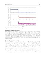
as shown in figure 7.a). One can observe that the pressure
c
p
has an initial step
decreasing,
(0)
c
p
k
p
k


, then an asymptotic increasing; meanwhile, the engine’s speed is
continuous asymptotic increasing.
One has also performed a simulation for a hypothetic engine, which has such a co-efficient
combination that 1
cpn
kk  ; even in this case the system is a stable one, but its stability
happens to be periodic, as figure 7.b) shows. One can observe that both the pressure and the
speed have small overrides (around 2.5% for n and 1.2% for
c
p

) during their stabilization.

Aircraft Gas-Turbine Engine’s Control Based on the Fuel Injection Control

317
The chosen RD-9 controller assures both stability and asymptotic non-periodic behavior for
the engine’s speed, but its using for another engine can produce some unexpected effects.

0
0.04
0.08
-0.04
-0.08
-0.12
-0.16
012
3
4
5
p
c
n
n
p
c
t [s]
0
0.05
0.10
-0.05

-0.10
-0.15
-0.20
012
3
4
5
p
c
n
n
p
c
t [s]
6
a)
b)

Fig. 7. System’s quality (system time response for

-step input)
4. Fuel injection controller with constant differential pressure
Another fuel injection control system is the one in figure 8, which assures a constant value of
the dosage valve’s differential pressure
ci
p
p

, the fuel flow rate amount
i

Q being
determined by the dosage valve’s opening.
As figure 8 shows, a rotation speed control system consists of four main parts: I-fuel pump with
plungers (4) and mobile plate (5); II-pump’s actuator with spring (22), piston (23) and rod (6);
III-differential pressure sensor with slide valve (17), preset bolt (20) and spring (18); IV-dosage
valve, with its slide valve (11), connected to the engine’s throttle through the rocking lever (13).

III
IV
n
I
3
4
5
6
7
8
9
10
11
12
0
0

y
FUEL TANK
i
p
0>z>0
0<x<0

c
p
II
2
1
13
16
15
14
17
19
20
21
23
2425
A
B
A
p
B
p
r
Q
sB
Q
sB
Q
sA
Q
22


ea
k
A
Q
B
Q
A
Q
S
T
O
P
i
Q
i
p
fuel
(to the combustor i njectors)
i
Q
i
p
p
Q
B
Q
c
p
0

>

>
0
18

es
k

Fig. 8. Fuel injection controller with constant differential pressure
rci
p
pp




Aeronautics and Astronautics

318
The system operates by keeping a constant difference of pressure, between the pump’s
pressure chamber (9) and the injectors’ pipe (10), equal to the preset value (proportional to
the spring (18) pre-compression, set by the adjuster bolt (20)). The engine’s necessary fuel
flow rate
i
Q and, consequently, the engine’s speed n, are controlled by the co-relation
between the
rci
p
pp differential pressure’s amount and the dosage valve’s variable slot

opening (proportional to the (13) rocking lever’s angular displacement

).
4.1 Mathematical model and transfer function
The non-linear mathematical model consists of the motion equations for each above
described sub-system In order to bring it to an operable form, assuming the small
perturbations hypothesis, one has to apply the finite difference method, then to bring it to a
non-dimensional form and, finally, to apply the Laplace transformer (as described in 3.2).
Assuming, also, that the fuel is a non-compressible fluid, the inertial effects are very small,
as well as the viscous friction, the terms containing m,

and

are becoming null.
Consequently, the simplified mathematical model form shows as follows





s1
p
BA px
pp
kx

, (53)

BAAB
pp

k
y
 , (54)


1
iz
ci
p
ic
p
ic
k
xpp z
kk

, (55)


1
ci p Qx
Qp
p
pQkkx
k


  
, (56)

ip
QQ k


 , (57)

pp
n
py
Qknk
y
. (58)
The model should be completed by the jet engine as controlled object equation


*
1
s1
MciHV
nkQ k p

  , (59)
where, for a constant flight regime, the term
*
1HV
k
p
becomes null.
The equations (53) to (59), after eliminating the intermediate arguments
,,,

ABc
ppp

,, ,,
iip
p
QQ
y
x , are leading to a unique equation:





s1
s1
s1 s1
Mcpn
MAB
AB
pic Qx p iz pic Qx p
px c py c px py
kk
kk
k
kk nkzkk
kkkk kk










  


.(60)

Aircraft Gas-Turbine Engine’s Control Based on the Fuel Injection Control

319
System’s transfer function is


sH

, with respect to the dosage valve’s rocking lever’s
position

. A transfer function with respect to the setting z,


s
z
H , is not relevant, because
the setting and adjustments are made during the pre-operational ground tests, not during
the engine’s current operation.

So, the main and the most important transfer function has the form below


10
2
210
s
s
ss
ff
H
ggg




, (61)
where the involved co-efficient are
102
,, ,
cp c pM
fkk fkkg









1
11
px py
pcpnM
AB pic Qx
kk
gkk
kk k





  





,


0
1
px py
cpn
AB
p
ic Qx
kk

gkk
kk k
 

. (62)
4.2 System quality
As the transfer function shows, the system is a static-one, being affected by static error.
One has studied/simulated a controller serving on a single spool jet engine (VK-1 type),
from the point of view of the step response, which means the system’s dynamic behavior for
a step input of the dosage valve’s lever’s angle

.
According to figure 9.a), for a step input of the throttle’s position

, as well as of the lever’s
angle

, the differential pressure
rci
p
pp

 has an initial rapid lowering, because of the
initial dosage valve’s step opening, which leads to a diminution of the fuel’s pressure
c
p
in
the pump’s chamber; meanwhile, the fuel flow rate through the dosage valve grows. The
differential pressure’s recovery is non-periodic, as the curve in figure 9.a) shows.
Theoretically, the differential pressure re-establishing must be made to the same value as

before the step input, but the system is a static-one and it’s affected by a static error, so the
new value is, in this case, higher than the initial one, the error being 4.2%. The engine’s
speed has a different dynamic behavior, depending on the
cpn
kk particular value.

0 1 2 3 4 5 6
t [s]
p
c
p
i
0 1 2 3 4 5
0
t [s]
n
a)
b)
-0.05
-0.04
-0.03
-0.02
-0.01
0
0.01
0.02
0.03
0.04
0.05
0.01

0.02
0.03
0.04
0.05
0.06
0.07
max
1.00
n


0.40
n


max
1.00
n


0.66
n


max
1.00
n


0.85

n



Fig. 9. System’s quality (system time response for

-step input)
One has performed simulations for a VK-1-type single-spool jet engine, studying three of its
operating regimes: a) full acceleration (from idle to maximum, that means from

Aeronautics and Astronautics

320
max
0.4 n to
max
n ); b) intermediate acceleration (from
max
0.65 n

to
max
n ); c) cruise
acceleration (from
max
0.85 n

to
max
n ).

If
1
cpn
kk 
, so the engine is a stable system, the dynamic behavior of its rotation speed n is
shown in figure 9.b). One can observe that, for any studied regime, the speed n, after an
initial rapid growth, is an asymptotic stable parameter, but with static error. The initial
growing is maxim for the full acceleration and minimum for the cruise acceleration, but the
static error behaves itself in opposite sense, being minimum for the full acceleration.
5. Fuel injection controller with commanded differential pressure
Unlike the precedent controller, where the differential pressure was kept constant and the
fuel flow rate was given by the dosage valve opening, this kind of controller has a constant
injection orifice and the fuel flow rate variation is given by the commanded differential
pressure value variation. Such a controller is presented in figure 10, completed by two
correctors (a barometric corrector VII and an air flow rate corrector VIII, see 5.3).
The basic controller has four main parts (the pressure transducer I, the actuator II, the
actuator’s feed-back III and the fuel injector IV); it operates together with the fuel pump V,
the fuel tank VI and, obviously, with the turbo-jet engine.

VI
P
FUEL TANK
I
IIIII
IV
V
1
2
3
4

5
6
7
8
9
10
11
12
13
14
15
16
17
18
19
l
1
l
2
l
3
l
4



0>u>0
0>x>0
0<y<0
Q

p
Q
T
Q
R
Q
S
Q
i
Q
S
Q
R
Q
z
Q
S
Q
x
p
p
p
R
p
i
p
i
p
p
p

i
p
e
p
p
20
l
6
l
5
VIII
21
22
23
24
VII
25
26
27
28
29
p
f
*
0<z<0
p
*
1
p
*

1
p
*
1
p
*
c
p
a
p
*
1

Fig. 10. Fuel injection controller with commanded differential pressure
rci
p
pp

 (basic
controller), with barometric corrector and air flow rate corrector

Aircraft Gas-Turbine Engine’s Control Based on the Fuel Injection Control

321
Controller’s duty is to assure, in the injector’s chamber, the appropriate
i
p
value, enough to
assure the desired value of the engine’s speed, imposed by the throttle’s positioning, which
means to co-relate the pressure difference

p
i
pp

to the throttle’s position (given by the 1
lever’s

-angle).
The fuel flow rate
i
Q , injected into the engine’s combustor, depends on the injector’s
diameter (drossel no. 15) and on the fuel pressure in its chamber
i
p
. The difference
p
i
pp
 ,
as well as
i
p
, are controlled by the level of the discharged fuel flow
S
Q through the
calibrated orifice 10, which diameter is given by the profiled needle 11 position; the profiled
needle is part of the actuator’s rod, positioned by the actuator’s piston 9 displacement.
The actuator has also a distributor with feedback link (the flap 13 with its nozzle or drossel
14, as well as the springs 12), in order to limit the profiled needle’s displacement speed.
Controller’s transducer has two pressure chambers 20 with elastic membranes 7, for each

measured pressure
p
p
and
i
p
; the inter-membrane rod is bounded to the transducer’s flap
4. Transducer’s role is to compare the level of the realized differential pressure
p
i
pp

to its
necessary level (given by the 3 spring’s elastic force, due to the (lever1+cam2) ensemble’s
rotation). So, the controller assures the necessary fuel flow rate value
i
Q , with respect to the
throttle’s displacement, by controlling the injection pressure’s level through the fuel flow
rate discharging.
5.1 System mathematical model and block diagram with transfer functions
Basic controller’s linear non-dimensional mathematical model can be obtained from the
motion equations of each main part, using the same finite differences method described in
chapter 3, paragraph 3.2, based on the same hypothesis.
The simplified mathematical model form is, as follows



111
s1
Rppx yy

p
kp kxk y

 
, (63)

22 2
p
pi RR Q p
p
k
p
k
p
kQ 
, (64)

y
RR ypp
y
k
p
k
p

, (65)

33ippy
p
k

p
k
y

, (66)

iii
Qk
p
 ,
u
uk


 , (67)
together with the fuel pump and the engine’s speed non-dimensional equations

p
pn
Qkn
, (68)


*
1
s1
mciHV
nkQ k
p


 
. (69)
where the used annotations are

2
16
00
1
,
4
2
PT d
pi
d
k
pp





0
44
2
,
R
xx
p
kd




2
0
1
4
2
i
Qi d
p
d
k
p




,
0
11 11
2
,
R
zz
p
kd




Aeronautics and Astronautics

322


2
7
7
00
1
,
4
2
RP
pR
d
k
pp






22
0
01 10
2
4tantan

4
i
sy
p
kdddy






,


22
01 10
0
1
4tantan
4
2
si
i
kdddy
p







,
11 11 0
0
1
() ,
2
zR s
R
kdzz
p




440
0
1
()
2
xR s
R
kdxx
p


 ,
0
0
u

kk
u


 ,
30
40
md
xd
rs
Sl
p
k
klx
 ,
0
0
u
u
k
x
 ,
0
0
p
dp
d
p
k
p

 ,
0
0
i
di
d
p
k
p
 ,

0
1
0
RP p
p
RP xR zR R
kp
k
kkk
p


,
2
1
R
y
zz
Sl

kl

 ,
10
1
02
zz
y
R
kl
y
k
p
l
 ,

0
1
0
xx
x
RP xR zR R
kx
k
kkk
p


,
0

0
Qi i
i
i
k
p
k
Q



0
2
0
PT i
p
RP PT
p
kp
k
kkp


,

0
2
0
RP R
R

RP PT
p
kp
k
kkp


,

0
2
0
p
Q
RP PT
p
Q
k
kk
p


,

0
120
RR
yR
rr
Sp

k
kk
y


,

0
120
Pp
yp
rr
Sp
k
kk
y


,

0
3
0
PT p
p
PT si Qi i
kp
k
kkkp



,

0
3
0
sy
y
PT si Qi i
ky
k
kkkp


,
0
0
0
p
pn
p
Q
n
k
Qn








. (70)
Furthermore, if the input signal u is considered as the reference signal forming parameter,
one can obtain the expression



ref
xd d d
xk
pp
  , (71)
where
re
f
d
p
is the reference differential pressure, given by
4
30
ref
rs
dr
md
kkl
pk
Slp





.
A block diagram with transfer functions, both for the basic controller and the correctors’
block diagrams (colored items), is presented in figure 11.


R
p
yR
k
+

y
1s
y



1y
k
1x
k

2R
k
yp
k
1p
k

xd
k
y
R
p
p
p
p
p
p
p
p
p
3p
k

3y
k
y

2p
k
i
p
i
p

c
k
i

Q
1s
m

1
n
pn
k
p
Q
2Q
k
i
k
i
p
i
p

dp
k
di
k
i
p
d
p
p
p
p

p
p
p
u
k

u

k
u
+
_
_
_
_
+
+
_
_
+
+
+
+
+
+
x
HV
k
*
1

p
R
p
i
p
n
fn
k
t f
k
yH
k
1t
k
*
f
p
*
f
p
_
+
_
*
1
p
*
1
p
*

1
p
n
d
p
y
n

Fig. 11. Block diagram with transfer functions

Aircraft Gas-Turbine Engine’s Control Based on the Fuel Injection Control

323
5.2 System quality
As figures 10 and 11 show, the basic controller has two inputs: a) throttle’s position - or
engine’s operating regime - (given by

-angle) and b) aircraft flight regime (altitude and
airspeed, given by the inlet inner pressure
*
1
p
). So, the system should operate in case of
disturbances affecting one or both of the input parameters


*
1
,
p


.
A study concerning the system quality was realized (using the co-efficient values for a VK-
1F jet engine), by analyzing its step response (system’s response for step input for one or for
both above-mentioned parameters). As output, one has considered the differential
pressure
d
p
, the engine speed n (which is the most important controlled parameter for a jet
engine) and the actuator’s rod displacement
y
(same as the profiled needle).
Output parameters’ behavior is presented by the graphics in figure 12; the situation
in figure 12.a) has as input the engine’s regime (step throttle’s repositioning) for a
constant flight regime; in the mean time, the situation in figure 12.b) has as input the
flight regime (hypothetical step climbing or diving), for a constant engine regime (throttle
constant position). System’s behavior for both input parameters step input is depicted in
figure 12.a).
One has also studied the system’s behavior for two different engine’s models: a stable-one
(which has a stabile pump-engine connection, its main co-efficient being 1
cpn
kk  , situation
in figure 13.a) and a non-stable-one (which has an unstable pump-engine connection
and 1
cpn
kk  , see figure 13.b).

-0.025
-0.02
-0.015

-0.01
-0.005
0
0.005
0.01
012345678910
t [s]
-0.0091
-0.0232
y(t)
n(t)
0.0087
p
d
(t)
-2
0
2
4
6
8
10
12
14
x 10
-3
012345678910
0,011
n(t)
y(t)

0.00015
-0.001
p
d
(t)
a)
b)
t [s]

Fig. 12. Basic system step response a) step input for




*
1
0p

; b) step input for
*
1
p



0


Concerning the system’s step response for throttle’s step input, one can observe that all
the output parameters are stables, so the system is a stable-one. All output parameters are

stabilizing at their new values with static errors, so the system is a static-one. However,
the static errors are acceptable, being fewer than 2.5% for each output parameter. The
differential pressure and engine’s speed static errors are negative, so in order to reach the
engine’s speed desired value, the throttle must be supplementary displaced (pushed).

Aeronautics and Astronautics

324
For immobile throttle and step input of
*
1
p
(flight regime), system’s behavior is similar (see
figure 12.b), but the static errors’ level is lower, being around 0.1% for
d
p
and for y , but
higher for
n (around 1.1%, which mean ten times than the others).
When both of the input parameters have step variations, the effects are overlapping, so
system’s behavior is the one in figure 13.a).
System’s stability is different, for different analyzed output parameters:
y
has a non-
periodic stability, no matter the situation is, but
d
p
and n have initial stabilization values
overriding. Meanwhile, curves in figures 12.a), 12.b) and 13.a) are showing that the engine
regime has a bigger influence than the flight regime above the controller’s behavior.

One also had studied a hypothetical controller using, assisting an unstable connection
engine-fuel pump. One has modified
c
k and
p
n
k
values, in order to obtain such a
combination so that 1
cpn
kk  . Curves in figure 13.b are showing a periodical stability for a
controller assisting an unstable connection engine-fuel pump, so the controller has reached
its limits and must be improved by constructive means, if the non-periodic stability is
compulsory.

-0.02
-0.015
-0.01
-0.005
0
0.005
0.01
0.015
012345678910
t [s]
-0.0121
n(t)
-0.0094
p
d

(t)
y(t)
0.0084
-0.06
-0.05
-0.04
-0.03
-0.02
-0.01
0
0.01
012345678910
t [s]
y(t)
0.00723
-
0.00362
p
d
(t)
-0,0538
n(t)
a)
b)

Fig. 13. Compared step response between a) stabile fuel pump-engine connection

1
cpn
kk 

and b) unstable fuel pump-engine connection


1
cpn
kk 

5.3 Fuel injection controller with barometric and air flow rate correctors
5.3.1 Correctors using principles
For most of nowadays operating controllers, designed and manufactured for modern jet
engines, their behavior is satisfying, because the controlled systems become stable and their
main output parameters have a non-periodic (or asymptotic) stability. However, some
observations regarding their behavior with respect to the flight regime are leading to the
conclusion that the more intense is the flight regime, the higher are the controllers’ static
errors, which finally asks a new intervention (usually from the human operator, the pilot) in
order to re-establish the desired output parameters levels. The simplest solution for this
issue is the flight regime correction, which means the integration in the control system of

Aircraft Gas-Turbine Engine’s Control Based on the Fuel Injection Control

325
new equipment, which should adjust the control law. These equipments are known as
barometric (bar-altimetric or barostatic) correctors.
In the mean time, some unstable engines or some unstable fuel pump-engine connections,
even assisted by fuel controllers, could have, as controlled system, periodic behavior, that
means that their output main parameters’ step responses presents some oscillations, as
figure 14 shows. The immediate consequence could be that the engine, even correctly
operating, could reach much earlier its lifetime ending, because of the supplementary
induced mechanical fatigue efforts, combined with the thermal pulsatory efforts, due to the
engine combustor temperature periodic behavior.

As fig. 14 shows, the engine speed
n and the combustor temperature
*
3
T (see figure 14.b), as
well as the fuel differential pressure
d
p
and the pump discharge slide-valve displacement
y

(see figure 14.a) have periodic step responses and significant overrides (which means a few
short time periods of overspeed and overheat for each engine full acceleration time).
The above-described situation could be the consequence of a miscorrelation between the
fuel flow rate (given by the connection controller-pump) and the air flow rate (supplied by
the engine’s compressor), so the appropriate corrector should limit the fuel flow injection
with respect to the air flow supplying.

0 2 4 6 8 10 12 14 16 18 20
x 10
-3
-10
-8
-6
-4
-2
0
2
4
6

8
y(t)
p
d
(t)
a)
t [s]
n(t)
T
3
(t)
*
0.039
-0.1
-0.08
-0.06
-0.04
-0.02
0
0.02
0.04
0.06
0 2 4 6 8 10 12 14 16 18 20
b)
t [s]

Fig. 14. Step response for an unstable fuel pump-engine connection assisted by a fuel
injection pressure controller
The system depicted in figure 10 has as main control equipment a fuel injection controller
(based on the differential pressure control) and it is completed by a couple of correction

equipment (correctors), one for the flight regime and the other for the fuel-air flow rates
correlation.
The correctors have the active parts bounded to the 13-lever (hemi-spherical lid’s support of
the nozzle-flap actuator’s distributor). So, the 13-lever’s positioning equation should be
modified, according to the new pressure and forces distribution.
5.3.2 Barometric corrector
The barometric corrector (position VII in figure 10) consists of an aneroid (constant pressure)
capsule and an open capsule (supplied by a
*
1
p
- total pressure intake), bounded by a
common rod, connected to the 13-lever.

Aeronautics and Astronautics

326
The total pressure
*
1
p
(air’s total pressure after the inlet, in the front of the engine’s
compressor) is an appropriate flight regime estimator, having as definition formula


**
1
,
HHc
pp M


 (72)
where
H
p
is the air static pressure of the flight altitude H,
*
c


inlet’s inner total pressure
lose co-efficient (assumed as constant),
H
M

air’s Mach number in the front of the inlet,
k  air’s adiabatic exponent and

1
2
1
1
2
k
k
HH
k
MM







.
The new equation of the 13-lever becomes



2
*
5
12 1
2
2
dd
d
d
RR pp s r r H a
yy
l
Sp Sp m k k y S p p
tl
t

   
, (73)
where
a
p

is the aneroid capsule’s pressure and, after the linearization and the Laplace
transformer applying, its new non-dimensional form becomes



*22
10
s2 s1
yR R yp p yH y y
kp kp kp T T yy


 
, (74)
and will replace the (65)-equation (see paragraph 5.2), where

*
10
5
1202
H
yH
rr
Sp
l
k
kk
y
l



.
5.3.3 Air flow-rate corrector
The air flow-rate corrector (position VIII in figure 10) consists of a pressure ratio transducer,
which compares the realized pressure ratio value for a current speed engine to the preset
value. The air flow-rate
a
Q is proportional to the total pressure difference
**
21
p
p

, as well as
to the engine’s compressor pressure ratio
*
*
2
*
1
c
p
p


. According to the compressor universal
characteristics, for a steady state engine regime, the air flow-rate depends on the pressure
ratio and on the engine’s speed



*
,
aac
QQ n


(Soicescu&Rotaru, 1999). The air flow-rate
must be correlated to the fuel flow rate
i
Q , in order to keep the optimum ratio of these
values. When the correlation is not realized, for example when the fuel flow rate grows
faster/slower than the necessary air flow rate during a dynamic regime (e.g. engine
acceleration/deceleration), the corrector should modify the growing speed of the fuel flow
rate, in order to re-correlate it with the realized air flow rate growing speed.
Modern engines’ compressors have significant values of the pressure ratio, from 10 to 30, so
the pressure difference
**
21
p
p

could damage, even destroy, the transducer’s elastic
membrane and get it out of order. Thus, instead of
*
2
p
-pressure, an intermediate pressure
*
f
p

, from an intermediate compressor stage “f”, should be used, the intermediate pressure
ratio
*
*
*
1
f
f
p
p


being proportional to
*
c

. The intermediate stage is chosen in order to obtain

Aircraft Gas-Turbine Engine’s Control Based on the Fuel Injection Control

327
a convenient value of
*
f
p
, around
*
1
4
p


. Both values of
*
f
p
and
*
2
p
are depending on
compressor’s speed (the same as the engine speed
n), as the compressor’s characteristic
shows; consequently, the air flow rate depends on the above-mentioned pressure (or on the
above defined
*
c

or
*
f

). The transducer’s command chamber has two drossels, which are
chosen in order to obtain critical flow through them (Soicescu&Rotaru, 1999), so the
corrected pressure
*
c
p
is proportional to the input pressure:

**

28
29
c
f
S
pp
S

, (75)
where
28 29
,SS
are 28 and 29-drossels’ effective area values. Consequently, the transducer
operates like a
*
c

-based corrector, correlating the necessary fuel flow-rate with the
compressor delivered air flow-rate. So, the corrector’s equations are:

**
22
()
p
pn
or
**
(),
ff
pp

n (76)
and become, after transformations,

*
ff
n
p
kn , (76’)

***
1
1
1
()
ffsff
p
xk kp p
k


  . (77)
The new form of (65)-equation becomes



2
**
6
12 1
2

2
dd
d
d
RR pp s r r mp c
yy
l
Sp Sp m k k y S p p
tl
t

    , (78)
where
mp
S is the transducer’s membrane surface area. After linearization and Laplace
transformer applying, its new non-dimensional form becomes





22 * *
011
s2 s1 ,
yy yRRypptfft
TT
y
k
p
k

p
k
p
k
p

 (79)
where

*
0
*
0
0
f
fn
f
p
n
k
n
p







,

*
0
*
28
29 0 26
mp f
f
r
fr
Sp
S
k
Sxk


 ,
 
**
010
66
1
1202 12102
,
mp f sf mp s
tf t
rr rrp
Spk Spk
ll
kk
kk

y
lkkk
y
l



. (80)
For a controller with both of the correctors, the (13)-lever equation results overlapping (73)
and (79)-equations, which leads to a new form





***22
111 0
s2 s1
yR R yp p yH tf f t y y
k
p
k
p
k
p
k
p
k
p
TT

yy


 , (81)

Aeronautics and Astronautics

328
which should replace the (65)-equation in the mathematical model (equations (63) to (69)).
The new block diagram with transfer functions is depicted in figure 11.
5.3.4 System’s quality
System’s behavior was studied comparing the step responses of a basic controller and the
step response (same conditions) of a controller with correctors. Fig. 15.a presents the step
responses for a controller with barometric corrector, when the engine’s regime is kept
constant and the flight regime receives a step modifying. The differential pressure
d
p

becomes non-periodic, but its static error grows, from -0.1% to 0.77% and changes its sign.
The profiled needle position
y behavior is clearly periodic, with a significant override, more
pulsations and a much bigger static error (1.85%, than 0.2%). Engine’s most important
output parameter, the speed
n, presents the most significant changes: it becomes non-
periodic (or remains periodic but has a short time smaller override), its static error
decreases, from 1.1% to 0.21% and it becomes negative.
However, in spite of the above described output parameter behavior changes, the
barometric corrector has realized its purpose: to keep (nearly) constant the engine’s speed
when the throttle has the same position, even if the flight regime (flight altitude or/and
airspeed) significantly changes.

Figure 15.b presents system’s behavior when an air flow-rate corrector assists the
controller’s operation. The differential pressure keeps its periodic behavior, but the profiled
needle’s displacement tends to stabilize non-periodic, which is an important improvement.
The main output non-dimensional parameters, the engine’s speed
n and the combustor’s
temperature
*
3
T have suffered significant changes, comparing to figure 14.b; both of them
tend to become non-periodic, their static errors (absolute values) being smaller (especially
for
n ). System’s time of stabilization became smaller (nearly half of the basic controller
initial value). So, the flow rate corrector has improved the system, eliminating the overrides
(potential engine’s overheat and/or overspeed), resulting a non-periodic stable system, with
acceptable static errors (5.5% for
n , 3% for
*
3
T ) and acceptable response times (5 to 12 sec).

p
d
(t)
y(t)
a)
-0.1
-0.08
-0.06
-0.04
-0.02

0
0.02
0.04
0.06
02468101214161820
T
3
(t)
*
n(t)
b)
with air flow rate corrector
without air flow rate corrector
-0.005
0
0.005
0.01
0.015
0.02
0.025
0.03
012345678910
t [s]
p
d
(t)
y(t)
-
0,0021
0.0077

0.0185
n(t)
t [s]
with air flow rate corrector
without air flow rate corrector

Fig. 15. Compared step response between a basic controller and a controller with
a) barometric corrector, b) air flow rate corrector

Aircraft Gas-Turbine Engine’s Control Based on the Fuel Injection Control

329
The barometric corrector is simply built, consisting of two capsules; its integration into the
controller’s ensemble is also accessible and its using results, from the engine’s speed point of
view, are definitely positives; new system’s step response shows an improvement, the
engine’s speed having smaller static errors and a faster stabilization, when the flight regime
changes. However, an inconvenience occurs, short time vibrations of the profiled needle (see
figure 15.b, curve
()
y
t ), without any negative effects above the other output parameters, but
with a possible accelerated actuator piston’s wearing out.
The air flow rate corrector, in fact the pressure ratio corrector, is not so simply built, because
of the drossels diameter’s choice, correlated to its membrane and its spring elastic
properties. However, it has a simple shape, consisting of simple and reliable parts and its
operating is safe, as long as the drossels and the mobile parts are not damaged.
Air flow-rate corrector’s using is more spectacular, especially for the unstable engines
and/or for the periodic-stable controller assisted engines; system’s dynamic quality changes
(its step response becomes non-periodic, its response time becomes significantly smaller).
6. Conclusions

Fuel injection is the most powerful mean to control an engine, particularly an aircraft jet
engine, the fuel flow rate being the most important input parameter of a control system.
Nowadays hydro-mechanical and/or electro-hydro-mechanical injection controllers are
designed and manufactured according to the fuel injection principles; they are
accomplishing the fuel flow rate control by controlling the injection pressure (or differential
pressure) or/and the dosage valve effective dimension.
Studied controllers, similar to some in use aircraft engine fuel controllers, even if they
operate properly at their design regime, flight regime’s modification, as well as transient
engine’s regimes, induce them significant errors; therefore, one can improve them by adding
properly some corrector systems (barometric and/or pneumatic), which gives more stability
an reliability for the whole system (engine-fuel pump-controller).
Both of above-presented correctors could be used for other fuel injection controllers and/or
engine speed controllers (for example for the controller with constant pressure chamber), if
one chooses an appropriate integration mode and appropriate design parameters.
7. References
Abraham, R. H. (1986). Complex dynamical systems, Aerial Press, ISBN #0-942344-27-8, Santa
Cruz, California, USA
Aron, I.; Tudosie, A. (2001). Jet Engine Exhaust Nozzle’s Automatic Control System,
Proceedings of the 17
th
International Symposium on Naval and Marine Education, pp. 36-
45, section III, Constanta, Romania, May 24-26, 2001
Jaw, L. C.; Mattingly, J. D. (2009).
Aircraft Engine Controls:Design System Analysis and Health
Monitoring,
Published by AIAA, ISBN-13: 978-1-60086-705-7, USA
Lungu, R.; Tudosie, A. (1997). Single Jet Engine Speed Control System Based on Fuel Flow
Rate Control,
Proceedings of the XXVII
th

International Conference of Technical Military
Academy in Bucuresti
, pp. 74-80, section 4, Bucuresti, Romania, Nov. 13-14, 1997
Lungu, R. (2000).
Flying Vehicles Automation, Universitaria, ISBN 973-8043-11-5, Craiova,
Romania

Aeronautics and Astronautics

330
Mattingly, J. D. (1996). Elements of Gas Turbine Propulsion, McGraw Hill, ISBN 1-56347-779-3,
New York, USA
Moir, I.; Seabridge, A. (2008).
Aircraft Systems. Mechanical, Electrical and Avionics Subsystems
Integration,
Professional Engineering Publication, ISBN-13: 978-1-56347-952-6, USA
Stoenciu, D. (1986).
Aircraft Engine Automation. Catalog of Automation Schemes, Military
Technical Academy Printing House, Bucuresti, Romania
Stoicescu, M.; Rotaru, C. (1999).
Turbo-Jet Engines. Characteristics and Control Methods,
Military Technical Academy Printing House, ISBN 973-98940-5-4, Bucuresti,
Romania
Tudosie, A. N. (2009). Fuel Injection Controller with Barometric and Air Flow Rate
Correctors,
Proceedings of the WSEAS International Conference on System Science and
Simulation in Engineering
(ICOSSSE'09), pp. 113-118, ISBN 978-960-474-131-1, ISSN
1790-2769, Genova, Italy, October 17-19, 2009.
12

Plasma-Assisted Ignition and Combustion
Andrey Starikovskiy
1
and Nickolay Aleksandrov
2
1
Princeton University
2
Moscow Institute of Physics and Technology
1
USA
2
Russia
1. Introduction
The history of application of thermally-equilibrium plasma for combustion control started
more than hundred years ago with IC engines and spark ignition systems. The same
principles still demonstrate high efficiency in different applications. Recently particular
interest appears in non-equilibrium plasma for ignition and combustion control
[Starikovskii, 2005; Starikovskaia, 2006]. The reason of the interest rise is new possibilities
for ignition and flame stabilization which are proposed by plasma-assisted approach. Over
the last decade, significant progress has been made in understanding the mechanisms of
plasma-chemistry interaction, energy redistribution in discharge plasma and non-
equilibrium initiation of combustion. Wide range of different fuels has been examined using
different types of discharges.
There are several mechanisms to affect a gas when using a discharge to initiate combustion
or stabilize a flame. There are two thermal mechanisms: 1) gas heating due to energy release
leads to an increase in the rates of chemical reactions; 2) inhomogeneous gas heating
generates flow perturbations and provokes turbulization and mixing. Non-thermal
mechanisms include 3) the effect of ionic wind (momentum transfer from electric field to the
gas due to space charge-electric field interaction); 4) the ion and electron drift in the electric

fields can lead to the additional fluxes of active radicals in the gradient flows; and 5)
excitation, dissociation and ionization of the gas by electron impact leads to the non-
equilibrium radical production and changes the kinetic mechanisms of ignition and
combustion. These mechanisms combined together or separately can provide an additional
authority to combustion control which is necessary for ultra-lean flames, high-speed flows,
cold low-pressure conditions of high-altitude GTE relight, detonation initiation in pulsed
detonation engines, distributed ignition control in HCCI engines and so on.
But, of course, the main interest in plasma technologies is connected with extreme
conditions like hypersonic aviation. A hypersonic aircraft that cruises at Mach 6 speed and ~
30 km altitude could travel 13,000 km in slightly over 2 hours, including the time needed for
takeoff, ascent, descent and landing [Bowcutt, 2009]. This is significant because almost all
major world city-pairs are separated by no more than 10,000-12,000 km. It is assumed that
the ability to travel such long distances in a short time would be valuable for the delivery of
time-critical cargo and for the relatively small percentage of passengers.
The advantage of short flight time, high speed and altitude would be promising to military
aircraft and missiles. An air-breathing hypersonic vehicle operates in multiple engine cycles

Aeronautics and Astronautics
332
and modes to reach scramjet operating speeds and could be used for the development of a
space transportation system that would allow cheap and flexible access to space. A typical
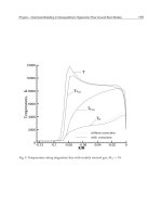
air-breathing hypersonic flight corridor with operation limits is presented in Figure 1
[Andreadis, 2005].


Fig. 1. Air-breathing hypersonic vehicle flight trajectory and operational limits [Andreadis,
2005].
Design challenges are dictated by flight conditions that become increasingly severe due to
the combination of internal duct pressure, skin temperature, and dynamic pressure loading
[Fry, 2004]. These constraints combination creates a narrow corridor of possible conditions

suitable for flight based on ram air compression. The lower boundary of this envelope is set
by thermal and structural limitations and is typically limited by a dynamic pressure of about
1 atm.
Relatively high dynamic pressure q is required, compared to a rocket, to provide adequate
static pressure in the combustor. The upper boundary is characterized as a region of low
combustion efficiency and narrow fuel/air ratio ranges thereby is restricted by combustion
stability in the engines (dynamic pressure limit is 0.25-0.5 atm).
The high Mach number (M > 15) edge of the envelope is a region of strong leading shock
waves, with strong dissociation and ionization of the gas in the shock layer. Here,
nonequilibrium flow can influence compression ramp flow, induce large leading-edge
heating rates, and reduce the efficiency of fuel injection and mixing and combustion. This
lead to dramatic performance decrease and puts another limitation on the possible flight
envelope for air-breathing hypersonic vehicles. On the contrary, at very low Mach numbers
(M < 3) the compression ratio due to flow deceleration is not enough for efficient ramjet
operation.
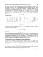
That is why in the low-speed regime (M = 0-3) the vehicle may utilize one of several possible
propulsion cycles such as a Turbine Based Combined Cycle (TBCC) with a bank of gas
turbine engines in the vehicle, or Rocket Based Combined Cycle (RBCC), with integrated
T
total
(K)
1
5
0
0
2
7
5
0
4

0
0
0
5
2
5
0
6
5
0
0
9
0
0
0
6
5
0
0
12
750
0.95
0.70
0.50
0.25
0.10
0.05
D
y
n

a
m
i
c

P
r
e
s
s
u
r
e
,

a
t
m
76,250
61,000
45,750
30,500
15,250
0
A
l
t
i
t
u

d
e
,

m

Plasma-Assisted Ignition and Combustion
333
rockets, internal or external to the engine, to accelerate the vehicle from takeoff to M ~ 3
(Figure 2). Above this point only ramjet/scramjet cycle can propose efficient operation.



Fig. 2. Propulsion efficiency and operating regimes [Andreadis, 2005]
The concept of scramjet is rather simple; (i) it has a shaped duct with an air inlet at its front
end and (ii) a constant-area or slightly divergent section where fuel is injected, mixed, and
burned. The section sharply diverges at its aft end to form internal and external nozzles.
Expansion of combustion products through the nozzle creates the thrust (Figure 3). The
proper shaping of the duct to provide efficient air compression, fuel-air mixing and
combustion, and gas expansion is a challenging task. To maximize the overall scramjet
performance, the duct should operate in concert with the vehicle upon which it is integrated
[Bowcutt, 2009]. This integration should take into account material limitations, fuel
characteristics, range of speed, flight attitude, and atmospheric pressure.



Fig. 3. Air-breathing supersonic combustion ramjet (scramjet), which provides a means of
efficient hypersonic propulsion [Bowcutt, 2009].
The scramjet engine can operate as a dual-mode ramjet in the Mach 3 to 6 regime along the
isolator capability limit to avoid inlet unstart and to remain within the structural limits

(Figure 2) [Andreadis, 2005]. As the vehicle continues to accelerate beyond Mach 7, the
combustion process is unable to separate the flow and the engine operates in scramjet mode