Aeronautics and Astronautics Part 12 doc

Creep Behaviors and Influence Factors of FGH95 Nickel-Base Superalloy

429

Fig. 7.7. Model of  precipitate shearing by coupled Shockley partials for creating
SISF/SESF pairs. After Hirth and Lothe (Unocic R. R. et al., 2008, as cited in Hirth J. P. &
Lothe J., 1968 )
The a<112> dislocations are hypothesized to originate from the interaction of two different
a<101> super- dislocations originating from different slip systems. For example:
a[011] + a[101]=a[112] (7.3)
Clearly, this model then requires a high symmetry orientation such that two slip systems
experience a relatively large shear stress.
In situ deformation at higher temperature gives rise to a distinctly different mode of
shearing in which the extended faults propagate continuously and viscously through both
particles and matrix. These extended faults are associated with partials that move in a
correlated manner as pairs. Koble (Koble M., 2001 ) induced that these partials may be
a/6<112> partials of the same Burgers vector, and that they may be traveling in parallel
{111} planes, as illustrated in Fig. 7.8. Without detailed confirmation of this hypothesis,
Kolbe further deduced that these were in fact micro-twins, and that the temperature
dependence of the process may be associated with recording that would ensure in the wake
of twinning a/6<112> partials as they traverse the  particles. The shear strain rate can be
expressed as follow:

)2/(ln[
)/(
22
2
tttpeff
tpord
tptptptp

fbf
bD
bb
x





(7.4)
Where, г
pt
is the energy of two layered pseudo-twin, and b
pt
is the magnitude of the Burgers
vector of the twinning partials, г
tt
is the energy of two layered true twin,

pt
is the density of
mobile twinning partials, D
ord
is the diffusion coefficient for ordering, x is the short range
diffusion length (assumed to be several nearest neighbor distances, or ~2b), f
2
is the volume
fraction of the secondary  precipitates, f
3
is the volume fraction of the tertiary  precipitates.

And the effective stress (

eff
) , in the presence of tertiary  precipitates, is given by:

3
2
p
t
eff
t
p
f
b


 (7.5)

Aeronautics and Astronautics

430
The experimental values of parameters such as dislocation density

pt
, volume fraction of
the secondary  precipitate that are critical to the prediction can be determined directly
from TEM observations. Disk alloys in this temperature regime typically exhibit the creep
curves having a minimum rate, with a prolonged increase of creep rate with time. As the
fine  phase volume fraction decreases during thermal exposure, it is possible that the
operation of 1/2[110] matrix dislocations becomes increasingly important. The coarse

microstructure (small value of f
3
) resulting from a slow cooling rate, the deformation is
dominated by 1/2<110> dislocation activated in the matrix, and SESF shearing in the
secondary  precipitates.


Fig. 7.8. Schematic representation of micro-twinning mechanism from shear by identical
Shockley partials (D) transcending both the  matrix and  precipitate in adjacent {111}
planes which then require atomic reordering in  to convert stacks of CSF into a true
twinned structure. After Kolbe (Koble M., 2001 )
8. Fracture features of the alloy during creep
8.1 Influence of solution temperature on fracture feature of alloy during creep
After the 1120 °C HIP alloy was solution treated at 1150 °C and isothermal quenched in
molten salt at 583 °C, the morphology of the alloy crept for different time under the applied
stress of 1034 MPa at 650 °C was shown in Fig. 8.1. The applied stress direction was marked
with the arrow in Fig. 8.1(a), after the alloy was crept for 40 h, some slipping traces appeared
on the surface of the sample, and some parallel slipping traces were displayed within the
same grain. Moreover, the various orientations of the slipping trace appeared within the
different grains. Besides, the kinking of the slipping traces appeared in the region of the
boundaries as marked by arrow in Fig. 8.1(a). After crept for 67 h up to rupture, the surface
morphology of the alloy was shown in Fig. 8.1(b), indicating that the amount of the slipping
trace increased as the creep went on, and the slipping traces were deepened to form the
slipping steps on the surface of the specimen. Moreover, the bended slipping traces
appeared in the boundary regions, as marked by longer arrow in Fig. 8.1(b), which was
Twinning Plane
Twin in matrix
Interface
True Twin
Pseudo Twin



D

D

D

D

Atomic reordering
C→A→B
B→C→A
A→B→C
C→A→A
B B B
A A A
C C C


Creep Behaviors and Influence Factors of FGH95 Nickel-Base Superalloy

431
attributed to the effect of the flow metal in the -free phase zone where is lower in strength.
Besides, the cracks were initiated in the distortion regions of slipping traces as marked by
shorter arrow in Fig. 8.1(b).


Fig. 8.1. Surface morphology of the alloy crept for different time up to fracture. (a) After
crept for 40 h, a few slipping traces appeared within the different grains, (b) after crept up to

fracture, significant amount of the slipping traces appeared on the sample surface, and
cracks appeared in the region near the boundary as marked by arrow


Fig. 8.2. After solution treated at 1160 °C, surface morphology of the alloy crept for different
time. (a) After crept for 60 h, a few slipping traces appeared within the different grains, (b)
after crept for 80 h, significant amount of the slipping traces appeared in the surface of the
sample
After 1120 °C HIP alloy was solution treated at 1160 °C and twice aged, the morphology of
the alloy crept for different time under the applied stress of 1034 MPa at 650 °C was shown
in Fig. 8.2. The direction of the applied stress was marked by arrows, after the alloy was
crept for 60 h, the morphology of the slipping traces on the sample surface was shown in
Fig. 8.2(a), which displayed the feature of the single orientation slipping appearing within
the different grains. And the intersected of the slipping traces appeared in the boundary
region as marked by arrow in Fig. 8.2(a), which indicated that the boundary may hinder the
3m
(b)
3m
(a)


5m
(b)
(a)
5m



Aeronautics and Astronautics

432
slipping of the traces to change their direction. When crept for 80 h, the quantities of the
slipping traces on the sample surface increased obviously, as shown in Fig. 8.2(b), and some
white blocky carbide particles were precipitated within the grains.
After solution treated at 1160 °C and twice aged, the surface morphology of the alloy crept
up to rupture under the applied stress of 1034 MPa at 650 °C was shown in Fig. 8.3. As the
creep went on, the quantities of the slipping traces increases gradually (the direction of the
applied stress shown in Fig. 8.3(a), which may bring out the stress concentration to promote
the initiation of the micro-cracks along the boundary which was vertical to the stress axis as
marked by the letter A and B in Fig. 8.3(a). In the other located region, the morphology of
the crack initiation was marked by letter C in Fig. 8.3(b), the micro-cracks displayed the non-
smooth surface as marked by arrow, and the white carbide particle was located in the crack,
it indicated that the carbide particles precipitated along the boundary may restrain the
cracks propagating along the boundaries to enhance the creep resistance of the alloy.


Fig. 8.3. Cracks initiated and propagated along the boundary. (a) Crack initiated along the
boundaries vertical to the stress axis, (b) crack propagated along the boundaries as marked
by arrow
After the alloy crept up to fracture, the morphology of the sample polished and eroded was
shown in Fig. 8.4. Some carbide particles were located in the boundaries as shown in Fig.
8.4(a), which may hinder the slipping of the dislocation for enhancing the creep resistance of
the alloy. Moreover, the unsmooth surface of the cracks appeared in the fracture regions as
marked by white arrow in Fig. 8.4(a). However, when no carbide particles were precipitated
along the boundaries, the crack after the alloy crept up to fracture displayed the smooth
surface as marked with the letter D and E in Fig. 8.4(b).
It may be thought by analysis that, although the carbide particles may hinder the
dislocations movement for improving the creep resistance of alloy, the carbides located in
the regions near the boundaries may bring about the stress concentration to promote the
initiation and propagation of the cracks along the boundary as marked with the arrow in

Fig. 8.4(a). Therefore, the fracture displayed the non-smooth surface due to the pinning
effect of the carbide particles precipitated along the boundaries to restrain the boundaries
slipping during creep. Though the carbide particles precipitated along the boundaries can
improve the cohesive strength of the boundaries, the micro-cracks are still initiated and
propagated along the boundaries, which suggests that the boundaries are still the weaker
regions for causing fracture of the alloy during creep.


10

m
(a)
B
A
m
(b)
C

Creep Behaviors and Influence Factors of FGH95 Nickel-Base Superalloy

433

Fig. 8.4. After solution treated at 1160 °C, surface morphology of the alloy crept up to
fracture. (a) Carbide particles near the crack along the boundary marked by arrow, (b)
morphology of cracks propagated along the boundary marked by arrow


Fig. 8.5. After solution treated at 1165 °C, surface morphology of the alloy crept for 9 h up to
fracture. (a) Crack initiated along the boundary as marked by arrow, (b) cracks propagated
along the boundary as marked by arrow

After solution treated at 1165 °C and aged, the surface morphology of the alloy crept for 9 h up
to rupture under the applied stress of 1034 MPa at 650 °C was shown in Fig. 8.5. A few
slipping trace appeared only on the surface of the alloy, and some micro-cracks were initiated
along the boundaries vertical to the applied stress axis, as marked by arrow in the Fig. 8.5(a).
As the creep went on, the morphology of the micro-crack propagated along the boundary was
shown in Fig. 8.5(b), in which the fracture of the alloy displayed the smooth surface. It may be
deduced according to the feature of the smooth fracture that the carbide films precipitated
along the boundaries has an important effect on decreasing the stress fracture properties of the
alloy. The carbide films were formed along the boundaries during heat treated, which reduced
the cohesive strength between the grains. Therefore, the micro-crack was firstly initiated along
the boundaries with the carbide films, and propagated along the interface between the carbide
films and grains, which resulted in the formation of the smooth surface on the fracture, and
decreased to a great extent the creep properties of the alloy.
5m
(b
E
D
σ

σ
(a
5

m
10m
(b)
10m
(a)



Aeronautics and Astronautics

434
After the alloy was crept for 9 h up to rupture under the applied stress of 1034 MPa at
650 °C, the surface morphology after the sample was polished and eroded was shown in
Fig. 8.6. The carbide films were continuously formed along the boundaries as marked
with the long arrow in Fig. 8.6(a), the direction of the applied stress was marked by
arrow, the micro-crack was initiated along the carbide film, as marked by shorter arrow in
Fig. 8.6(a). As the creep went on, the morphology of the crack propagated along the
boundaries was shown in Fig. 8.6(b), the fracture after the crack was propagated
displayed the smooth surface, and the white carbide film was reserved between the
tearing grains marked by arrow in Fig. 8.6(b), which displayed an obvious feature of the
intergranular fracture of the alloy during creep. It can be thought by analysis that the
carbide films precipitated along the boundaries, during heat treated, possessed the hard
and brittle features and weakened the cohesive strength between the grains. Therefore,
the micro-crack was firstly initiated along the carbide films and propagated along the
interface between the grains and carbide films, which resulted in the formation of the
smooth surface on the fracture, so the alloy had the lower toughness and shorter creep
lifetime. Moreover, it was identified by means of composition analysis under SEM/EDS
that the elements Nb, Ti, C and O were rich in the white particles on the surface of the
samples, as shown in Fig. 8.2, Fig. 8.3 and Fig. 8.5, respectively, therefore, it is thought
that the white particles on the surface of the samples are the oxides of the elements Nb, Ti
and C.


Fig. 8.6. After solution treated at 1165 °C, surface morphology of the alloy crept for 9 h up to
fracture. (a) Crack initialed along the boundary marked by arrow, (b) morphology of cracks
propagated along the boundary marked by arrow.
8.2 Influence of quenching temperatures on fracture feature of alloy during creep

After the 1180°C HIP alloy was solution treated at 1150 °C and cooled in oil bath at 120 °C,
the morphologies of the alloy crept for 260 h up to rupture under the applied stress of 984
MPa at 650 °C were shown in Fig. 8.7. If the PPB region between the powder particles was
regard as the grain boundaries as shown in Fig. 8.7(a), the grain boundaries after the alloy
was crept up to rupture were still wider, and the ones were twisted into the irregular piece-
like shape as marked by arrow in Fig. 8.7(a).
8m
(a)


(b)
8m

Creep Behaviors and Influence Factors of FGH95 Nickel-Base Superalloy

435

Fig. 8.7. Microstructure of alloy after crept up to fracture under the applied stress of 984
MPa at 650 °C. (a) Wider grain boundaries broken into the irregular shape as marked by
arrow, (b) traces with double orientations slipping feature appeared within the grain as
marked by arrows, (c) finer particles precipitated along the slipping traces
Some irregular finer grains were formed in the boundary regions, and displaying a bigger
difference in the grain sizes. Some coarser  precipitates were precipitated in the boundaries
region in which the creep resistance is lower due to the spareness of the finer  phase. The
severed deformation of the alloy occurred firstly in the boundary regions during high stress
creep, which resulted in the boundaries broken into the irregular piece-like shape. At the
same time of the severed deformation, the traces with double orientations slipping feature
appeared within the grains as marked by arrows in Fig. 8.7(b), and some particles were
precipitated in the boundaries region as marked by short arrow in Fig. 8.7(b). Moreover, the
finer white particles were precipitated in the regions of the double orientations slipping

traces as marked by arrows in Fig. 8.7(c), and the white particles were distinguished as the
carbides containing the elements Nb, Ti and C by means of SEM/EDS composition analysis.


Fig. 8.8. Microstructure after the molten salt cooled alloy crept up to fracture under the
applied stress of 1034 MPa at 650 °C. (a) Traces of the double orientations slipping appeared
within the grains, (b) magnified morphology of the slipping traces
(b
10

m
10m
(c
(a
20m
10m
(b
20m
(a)

Aeronautics and Astronautics

436
After solution treated at 1150 °C, and cooled in molten salt at 583 °C, the morphology of the
alloy crept for 67 h up to rupture under the applied stress of 1034 MPa at 650 °C was shown
in Fig. 8.8. This indicated that the traces with the double orientations slipping feature
appeared within the grain, and the various orientations of the slipping traces appeared in
the different grains, thereinto, the directions of the thicker and fine traces were marked by
the arrows, respectively, in Fig. 8.8(a). Moreover, the traces with the cross-slipping feature
were marked by shorter arrow in Fig. 8.8(a).

8.3 Analysis on fracture features during creep
After solution treated at various temperatures, the alloy had different creep properties due
to the difference of microstructure as shown in Table 6.2. When solution treated at 1150 °C,
the alloy possessed a uniform grain size and wider PPB regions between the grains.
Moreover, some coarser  precipitates were distributed along the PPB regions in which no
fine -phase was precipitated in the regions near the coarser -phase, as shown in Fig.
4.2(a), the regions possessed a lower creep strength due to the cause of the -free phase
zone. After the alloy was solution treated at 1160 °C and twice aged, the coarser 
precipitates along the boundary regions disappeared, the boundaries appeared obviously in
between the grains. And the cohesive strength between the grains was obviously improved
due to the pinning effect of the fine carbide particles, as shown in Fig. 4.3(b), therefore, the
alloy displayed a better creep resistance and longer the lifetime.
After the 1120 °C HIP alloy was solution treated at 1160 °C and twice aged, the alloy was
crept for 104 h up to fracture under the applied stress of 1034 MPa at 650 °C, the fracture
after the alloy was crept up to rupture displayed the initiating and propagating feature of
the cuneiform crack as marked by letters A and B in Fig. 8.3. The schematic diagram of the
crack initiated along the triangle boundary is shown in Fig. 8.9, where σ
n
is the normal
stress applied on the boundary, L is the boundary length, h is the displacement of the
cuneiform crack opening,

is the crack length, θ is the inclined angle of the adjacent
boundaries.


Fig. 8.9. Schematic diagram of the crack initiated along the triangle boundary
Under the action of the applied stress, significant amount of the activated dislocations are
piled up the regions near the boundary to bring the stress concentration, which results in
the initiation of the crack in the region near the triangle boundary, and the crack is



Creep Behaviors and Influence Factors of FGH95 Nickel-Base Superalloy

437
propagated along the boundary as the creep goes on. Thereinto, the critical length (

C
) of
the instable crack propagated along the boundary can be expressed as follows (Yoo M. H.,
1983).

2
2(1 )
c
f
Gh
a




(8.1)
Where, G is shearing modulus, ν is Poisson ratio,

f
is the crack propagating work, h is the
displacement of the cuneiform crack opening. This indicates that critical length (

c

) of the
instable crack propagated along the boundary increases with the displacement of the crack
opening, and is inversely to the crack opening work. Thereinto, the displacement of the
crack opening increases with the creep time, which can be express as follows:

4sin
() 1 exp( )
B
B
t
ht

 



  





(8.2)
Where h
w
=(is the max displacement of the crack opening, τ is the resolving shear stress
component applied along the boundary, t is the time of the crack propagation,

B
is the

boundary thickness,

B
is the sticking coefficient of the boundary slipping, β is the material
constant.
The Eq. (8.2) indicates that the displacement of the crack opening (h) increases with the time
and length of crack propagation. When two cuneiform-like cracks on the same boundary are
joined each other due to their propagation, the intergranular rupture of the alloy occurs to
form the smooth surface on the fracture. The schematic diagram of two cuneiform-like
cracks initiated and propagated along the boundary for promoting the occurrence of the
intergranular fracture is shown in Fig. 8.10. If the carbide particles are dispersedly
precipitated along the boundaries, the ones may restrain the boundaries slipping for
improving the creep resistance of the alloy to form the non-smooth surface on the fracture,
as marked by arrow in Fig. 8.3(b).
After solution treated at 1165 °C and twice aged, the grain size of the alloy increased
obviously, and the carbide films were formed along the boundaries as shown in Fig. 4.4,
which weakened the cohesive strength between the grains. Therefore, the cracks were easily
initiated and propagated along the boundaries adjoined to the carbide films, which may
sharply reduce the lifetime and plasticity of the alloy during creep.


Fig. 8.10. Schematic diagram of the cuneiform-like cracks initiated and propagated along the
boundary. (a) Triangle boundary, (b) initiation of the cuneiform-like crack, (c) propagation
of the crack along the boundary
A
B C
D
(a)
A
B

C
D
(b)
B
A
C
D
(c)

Aeronautics and Astronautics

438
Because the boundaries and the carbide particles can effectively hinder the dislocation
movement, and especially, the carbide particles can improve the cohesive strength between
the grains and restrain the boundaries slipping during creep, therefore, it may be concluded
that the carbide particles precipitated along the boundaries have an important effect on
improving the creep resistance of the alloy. Although the carbide particles precipitated
along the boundaries can improve the strength of the boundaries, the micro-cracks are still
initiated and propagated along the boundaries, which suggests that the boundaries are still
the weaker regions for causing fracture of the alloy during creep. And once, the carbide is
continuously precipitated to form the film along the boundary, which may weaken the
cohesive strength between the grains to damage the creep lifetimes of the alloy. The analysis
is in agreement with the experimental results stated above.
When the alloy was solution treated at 1150 °C and cooled in oil bath at 120 °C, the carbon
atoms were supernaturally dissolved in the matrix of the alloy due to quenching at lower
temperature. The concentration supersaturation in the alloy promoted the carbon atoms for
precipitating in the form of the fine carbide particles during creep under the applied higher
tensile stress at 650 °C, in especially, the slipping trace regions support a bigger extruding
stress for inducing the carbon atoms to precipitate in the form of the fine carbide particles
along the slipping traces as shown in Fig. 8.7(c). This is thought to be a main reason of the

fine carbides precipitated along the slipping traces.
On the other hand, when the alloy was solution treated at 1150 °C and cooled in molten salt
at 583 °C, although the slipping traces appeared still in the matrix of the alloy during creep,
no fine carbide particles were precipitated along the slipping traces, as shown in Fig. 8.8,
due to the concentration supersaturation of the carbon atoms in the matrix is lower than the
one of the alloy cooled in oil bath at 120 °C.
9. Conclusion
By means of hot isostatic pressing and heat treated at different temperatures, creep curves
measurement and microstructure observation, an investigation had been made into the
influence of hot isostatic pressing and heat treatment on the microstructure and creep
behaviors of FGH95 nickel-base superalloy. Moreover, the deformation and fracture
mechanisms of the alloy were discussed. The conclusions were mainly listed as follows:
1.
When the alloy was hot isostatic pressed below the dissolving temperature of phase,
as the HIP temperature increased, the size and amount of primary coarse phase
decreased gradually in the PPB regions, and the size of the grains was equal to the one
in the previous powder particles. With the HIP temperature increased to 1180°C, the
coarse phase in the PPB was completely dissolved, and the grain of the alloy grew up
obviously.
2.
When the solution temperature was lower than the dissolving temperature of  phase,
after solution treated at 1140 °C, finer  phase was dispersedly precipitated within the
grains, and some coarser  precipitates were distributed in the wider boundary regions
where appeared the depleted zone of the fine -phase. With the solution temperature
increased, the amounts of the coarser  phase and the zone of -free phase decreased
gradually.
3.
After solution temperature increased to 1160 °C, the coarser  phase in the alloy was
fully dissolved, the fine secondary  phase with high volume fraction was dispersedly

Creep Behaviors and Influence Factors of FGH95 Nickel-Base Superalloy

439
distributed within the grains, and the particles of (Nb, Ti)C

carbide were precipitated
along the boundaries. When the alloy was solution treated at 1165 °C, the size of the
grains was obviously grown up, and the carbides were continuously precipitated to
form the films along the boundaries.
4.
During long term aging in the ranges of 450 °C and 550 °C, no obvious change in the
grain size was detected in the alloy as the aging time prolonged, but the  phase grew
up slightly. With the aging time prolonging, the lattice parameters of the  and  phases
increases slightly, but the misfit of   phases decreased slightly.
5.
Under the applied stress of 1034 MPa at 650 °C, the solution treated alloy cooled in
molten salt displayed a better creep resistance. In the ranges of the applied
temperatures and stresses, the creep activation energy of the alloy was measured to be
Q = 590.320 kJ/mol.
6.
The deformation mechanisms of the alloy during creep were the twinning, dislocations
by-passing or shearing into the  phase. The <110> super-dislocations shearing into the
 phase may be decomposed to form the configuration of (1/3)<112> super-Shockleys
partial plus stacking fault.
7.
During creep, the deformed features of the solution treated alloy cooled in oil bath was
that the double orientation slipping of dislocations were activated, and the fine carbide
particles were precipitated along the regions of the slipping traces. And the depleted
zone of the fine  phase was broken into the irregular piece-like shape due to the severe
plastic deformation.

8.
The deformed features of the alloy treated in molten salt were that the twinning and
dislocation tangles were activated in the matrix of the alloy. Thereinto, the fact that the
particles-like carbides were dispersedly precipitated within the grains and along the
boundary might effectively restrain the dislocation slipping and hinder the dislocations
movement, which is one important factor of the alloy possessing the better creep
resistance and the longer creep lifetime.
9.
In the later stage of creep, the slipping traces with the single or double orientations
features appeared on the surface of the alloy. As the creep went on, the amount of the
slipping traces increased to bring about the stress concentration, which might promote
the initiation and propagation of the micro-cracks along the boundaries, this was
thought to be the main fracture mechanism of the alloy during creep.

10. References
Domingue J. A., Boesch W. J., Radavich J. F (1980). Superalloys1980. pp.335 – 344.
Flageolet B.; Jouiad M.; Villechaise P., et al. (2005). Materials Science and Engineering A, Vol.
399, pp. 199 – 205, ISSN: 0921 – 5093.
Hirth J. P. & Lothe J. (1968). Theory of Dislocations, 2
nd
ed., Wiley, New York, p.319
Hu B. F., Chen H. M., Li H. Y., et al. (2003). Journal of Materials Engineering, No.1, pp. 6 – 9,
ISSN: 1001 – 4381.
Hu B. F., Yi F. Zh., et al. (2006). Journal of University of Science and Technology Beijing, Vol.28,
No.12, pp. 1121 – 1125, ISSN: 1001 – 053X.
Jia CH. CH., Yin F. ZH., Hu B. F., et al. (2006). Materials Science and Engineering of Powder
Metallurgy, Vol.11, No.3, pp.176 – 179, ISSN: 1673 – 0224
Klepser C. A (1995). Scripta Metallurgical, Vol.33, No.4, pp. 589 – 596, ISSN: 1359 – 6462.

Aeronautics and Astronautics

440
Kovarik L. , Unocic R. R. , Li J. , et al. (2009). Journal of the Minerals, Vol. 61, No.2, pp. 42 – 48,
ISSN: 1047 – 4838.
Koble M (2001). Materials Science and Engineering A, Vol. 319-321, PP. 383 – 387, ISSN: 0921 –
5093.
Lherbier L.W. & Kent W. B ( 1990). The International Journal of Powder Metallurgy, Vol.26,
No.2, pp. 131 – 137, ISBN: 0361 – 3488.
Liu D. M., Zhang Y., P. Liu Y., et al. (2006). Powder Metallurgy Industry, Vol.16, No.3 pp. 1-5,
ISSN: 1006 – 6543.
Lu Z. Z., Liu C. L., Yue Z. F (2005). Materials Science and Engineering A, Vol. 395, pp. 153 –
159, ISSN: 0921 – 5093.
Park N. K. & Kim I. S (2001). Journal of Materials Processing Technology, Vol. 111, No.2, pp. 98
– 102, ISSN: 0924 – 0136.
Paul L (1988). Powder Metallurgy Superalloys, pp. 27 – 36.
Raujol S., Pettinari F., Locq D., et al. (2004). Materials Science and Engineering A, Vol. 387 –
389, pp.678 – 82, ISSN: 0921 – 5093.
Terzi S., Couturier R., Guetal L., et al. (2008). Materials Science and Engineering A, Vol. 483-
484, pp. 598 – 601, ISSN: 0921 – 5093.
Viswanathan G. B., Sarosi P. M., Henry M. F., et al. (2005). Acta Materialia, Vol.53, pp.
3041~3057, ISSN: 1359 – 6454.
Unocic R. R., Viswanathan G. B., Sarosi P. M., et al. (2008). Materials Science and Engineering
A, Vol. 483 – 484, pp. 25 – 32, ISSN: 0921 – 5093
Wang P., Dong J. X., Yang L., et al. (2008). Material Review, Vol.22, No.6, pp. 61 – 64, ISSN:
1005 – 023X.
Yoo M. H. & Trinkaus H (1983). Metall. Trans., Vol. 14, No.4, pp. 547 – 561, ISSN: 1073-
5623.
Zainul H. D (2007). Materials and Design, Vol.28, pp.1664 – 1667, ISSN: 0261 – 3069.
Zhang J. SH (2007). High Temperature Deformation and Fracture of Material. Beijing: Science
Press, pp. 102 – 105, ISBN: 978 – 7 – 03 – 017774 – 2.

Zhang Y. W., Zhang Y., Zhang F. G., et al. (2002). Transactions of Materials and Heat Treatment,
Vol.23, No.3, pp. 72 – 75, ISSN: 1009 – 6264.
Zhou J. B., Dong J. X., Xu Zh. Ch., et al. (2002). Heat Treatment of Metals, vol.27, No.6, pp.30 –
32. ISSN: 0254 – 6051.
15
Multi-Dimensional Calibration of Impact Models
Lucas G. Horta, Mercedes C. Reaves,
Martin S. Annett and Karen E. Jackson
NASA Langley Research Center, Hampton, VA
USA
1. Introduction
As computational capabilities continue to improve and the costs associated with test
programs continue to increase, certification of future rotorcraft will rely more on
computational tools along with strategic testing of critical components. Today, military
standards (MIL-STD 1290A (AV), 1988) encourage designers of rotary wing vehicles to
demonstrate compliance with the certification requirements for impact velocity and volume
loss by analysis. Reliance on computational tools, however, will only come after rigorous
demonstration of the predictive capabilities of existing computational tools. NASA, under
the Subsonic Rotary Wing Program, is sponsoring the development and validation of such
tools. Jackson (2006) discussed detailed requirements and challenges associated with
certification by analysis. Fundamental to the certification effort is the demonstration of
verification, validation, calibration, and algorithms for this class of problems. Work in this
chapter deals with model calibration of systems undergoing impact loads.
The process of model calibration, which follows the verification and validation phases,
involves reconciling differences between test and analysis. Most calibration efforts combine
both heuristics and quantitative methods to assess model deficiencies, to consider
uncertainty, to evaluate parameter importance, and to compute required model changes.
Calibration of rotorcraft structural models presents particular challenges because the
computational time, often measured in hours, limits the number of solutions obtainable in a
timely manner. Oftentimes, efforts are focused on predicting responses at critical locations

as opposed to assessing the overall adequacy of the model. For example (Kamat, 1976)
conducted a survey, which at the time, studied the most popular finite element analysis
codes and validation efforts by comparing impact responses from a UH-1H helicopter drop
test. Similarly, (Wittlin and Gamon, 1975) used the KRASH analysis program for data
correlation of the UH-1H helicopter. Another excellent example of a rotary wing calibration
effort is that of (Cronkhite and Mazza, 1988) comparing results from a U.S. Army composite
helicopter with simulation data from the KRASH analysis program. Recently, (Tabiei,
Lawrence, and Fasanella, 2009) reported on a validation effort using anthropomorphic test
dummy data from crash tests to validate an LS-DYNA (Hallquist, 2006) finite element
model. Common to all these calibration efforts is the use of scalar deterministic metrics.
One complication with calibration efforts of nonlinear models is the lack of universally
accepted metrics to judge model adequacy. Work by (Oberkampf et al., 2006) and later
(Schwer et al., 2007) are two noteworthy efforts that provide users with metrics to evaluate
nonlinear time histories. Unfortunately, seldom does one see them used to assess model

Aeronautics and Astronautics
442
adequacy. In addition, the metrics as stated in (Oberkampf et al., 2006) and (Schwer et al.,
2007) do not consider the multi-dimensional aspect of the problem explicitly. A more
suitable metric for multi-dimensional calibration exploits the concept of impact shapes as
proposed by (Anderson et al., 1998) and demonstrated by (Horta et al., 2003). Aside from the
metrics themselves, the verification, validation, and calibration elements, as described by
(Roache, 1998; Oberkampf, 2003; Thacker, 2005; and Atamturktur, 2010), must be adapted to
rotorcraft problems. Because most applications in this area use commercially available
codes, it is assumed that code verification and validation have been addressed elsewhere.
Thus, this work concentrates on calibration elements only. In particular, this work
concentrates on deterministic input parameter calibration of nonlinear finite element
models. For non-deterministic input parameter calibration approaches, the reader is
referred to (Kennedy and O‘Hagan, 2001; McFarland et al., 2008).
Fundamental to the success of the model calibration effort is a clear understanding of the

ability of a particular model to predict the observed behavior in the presence of modeling
uncertainty. The approach proposed in this chapter is focused primarily on model
calibration using parameter uncertainty propagation and quantification, as opposed to a
search for a reconciling solution. The process set forth follows a three-step approach. First,
Analysis of Variance (ANOVA) as described in work by (Sobol et al., 2007; Mullershon and
Liebsher, 2008; Homma and Saltelli, 1996; and Sudret, 2008) is used for parameter selection
and sensitivity. To reduce the computational burden associated with variance based
sensitivity estimates, response surface models are created and used to estimate time
histories. In our application, the Extended Radial Basis Functions (ERBF) response surface
method, as described by (Mullur, 2005, 2006) has been implemented and used. Second, after
ANOVA estimates are completed, uncertainty propagation is conducted to evaluate
uncertainty bounds and to gage the ability of the model to explain the observed behavior by
comparing the statistics of the 2-norm of the response vector between analysis and test. If
the model is reconcilable according to the metric, the third step seeks to find a parameter set
to reconcile test with analysis by minimizing the prediction error using the optimization
scheme proposed (Regis and Shoemaker 2005). To concentrate on the methodology
development, simulated experimental data has been generated by perturbing an existing
model. Data from the perturbed model is used as the target set for model calibration. To
keep from biasing this study, changes to the perturbed model were not revealed until the
study was completed.
In this chapter, a description of basic model calibration elements is described first followed
by an example using a helicopter model. These elements include time and spatial multi-
dimensional metrics, parameter selection, sensitivity using analysis of variance, and
optimization strategy for model reconciliation. Other supporting topics discussed are
sensor placement to assure proper evaluation of multi-dimensional orthogonality metrics,
prediction of unmeasured responses from measured data, and the use of surrogates for
computational efficiency. Finally, results for the helicopter calibrated model are presented
and, at the end, the actual perturbations made to the original model are revealed for a quick
assessment.
2. Problem formulation

Calibration of models is a process that requires analysts to integrate different
methodologies in order to achieve the desired end goal which is to reconcile prediction

Multi-Dimensional Calibration of Impact Models
443
with observations. Although in the literature the word “model” is used to mean many
different forms of mathematical representations of physical phenomena, for our purposes,
the word model is used to refer to a finite element representation of the system. Starting
with an analytical model that incorporates the physical attributes of the test article, this
model is initially judged based on some pre-established calibration metrics. Although
there are no universally accepted metrics, the work in this paper uses two metrics; one
that addresses the predictive capability of time responses and a second metric that
addresses multi-dimensional spatial correlation of sensors for both test and analysis data.
After calibration metrics are established, the next step in the calibration process involves
parameter selection and uncertainty estimates using engineering judgment and available
data. With parameters selected and uncertainty models prescribed, the effect of parameter
variations on the response of interest must be established. If parameter variations are
found to significantly affect the response of interest, then calibration of the model can
proceed to determine a parameter set to reconcile the model. These steps are described in
more detail, as follows.
2.1 Time domain calibration metrics
Calibration metrics provide a mathematical construct to assess fitness of a model in a
quantitative manner. Work by (Oberkampf, 2006) and (Schwer, 2007) set forth scalar
statistical metrics ideally suited for use with time history data. Metrics in terms of mean,
variance, and confidence intervals facilitate assessment of experimental data, particularly
when probability statements are sought. For our problem, instead of using response
predictions at a particular point, a vector 2-norm (magnitude of vector) of the system
response is used as a function of time. An important benefit of using this metric is that it
provides for a direct measure of multi-dimensional closeness of two models. In addition,
when tracked as a function of time, closeness is quantified at each time step.

Because parameter values are uncertain, statistical measures of the metric need to be used to
conduct assessments. With limited information about parameter uncertainty, a uniform
distribution function, which is the least informative distribution function, is the most
appropriate representation to model parameter uncertainty. This uncertainty model is used
to create a family of N equally probable parameter vectors, where N is arbitrarily selected.
From the perspective of a user, it is important to know the probability of being able to
reconcile measured data with predictions, given a particular model for the structure and
parameter uncertainty. To this end, let
2
(, ) (, )Qt
p
vt
p
 be a scalar time varying function,
in which the response vector
v is used to compute the 2-norm of the response at time t, using
parameter vector p. Furthermore, let
() min (, )
p
tQt
p



be the minimum value over all
parameter variations, and let
() max (, )
p
tQtp



 be the maximum value. Using these
definitions and N LS-DYNA solutions corresponding to equally probable parameter vectors,
a calibration metric can be established to bound the probability of test values falling outside
the analysis bounds as;

1
M=Prob( () () () ()) 1/
ee
tQtQt t N



 (1)
where
()
e
Qt
is the 2-norm of responses from the experiment. Note that N controls tightness
of the bounds and also the number of LS-DYNA solutions required.

Aeronautics and Astronautics
444
The use of norms, although convenient, tends to hide the spatial relationships that exist
between responses at different locations in the model. In order to study this spatial multi-
dimensional dependency explicitly, a different metric must be established.
2.2 Spatial multi-dimensional calibration metric
Spatial multi-dimensional dependency of models has been studied in classical linear dynamic
problems in terms of mode shapes or eigenvectors resulting from a solution to an eigenvalue
problem. Unfortunately, the nonlinear nature of impact problems precludes use of any simple

eigenvalue solution scheme. Alternatively, an efficient and compact way to study the spatial
relationship is by using a set of orthogonal impact shape basis vectors. Impact shapes,
proposed by (Anderson, 1998 and later by Horta, 2003), are computed by decomposing the
time histories using orthogonal decomposition. For example, time histories from analysis or
experiments can be decomposed using singular value decomposition as

1
(,) () ()
n
ii i
i
y
xt xg t




(2)
In this form, the impact shape vector
i

sized m x 1, contains the spatial distribution
information for m sensors, g(t) contains the time modulation information,

contains scalar
values with shape participation factors, and n is the number of impact shapes to be included
in the decomposition, often truncated based on allowable reconstruction error. Although Eq.
(2) is written in continuous time form, for most applications, time is sampled at fixed
intervals such that
tkT



where the integer k=0,…,L and
T

is the sample time. From Eq.
(2), the fractional contribution of the i
th
impact shape to the total response is proportional to
i

, defined as;

1
n
ii l
l





(3)
Mimicking the approach used in classical dynamic problems, impact shapes can now be
used to compare models using orthogonality. Orthogonality, computed as the dot product
operation of vectors (or matrices), quantifies the projection of one vector onto another. If the
projection is zero, vectors are orthogonal, i.e., uncorrelated. This same idea applies when
comparing test and analysis impact shapes. Numerically, the orthogonality metric is
computed as;

2
T
M




(4)
where


is sized m x l with l measured impact shapes at m locations and


, sized m x l,
are shapes computed using simulation data. Note that both


and


are normalized
matrices such that
T
I



and
T

I



. Because individual impact shape vectors are
stacked column-wise, metric
2
M
is a matrix sized l x l with diagonal values corresponding
to the vector projection numerical value. If vectors are identical then their projection equals
1. Consequently, when evaluating models, multi-dimensional closeness with experiment is
judged based on similarity of impact shapes and shape contributions. Two direct benefits of
using impact shapes are discussed in the next two sections.

Multi-Dimensional Calibration of Impact Models
445
2.2.1 Algorithm for response interpolation
Adopting impact shapes as a means to compare models has two advantages. First, it allows
for interpolation of unmeasured response points, and second, it provides a metric to
conduct optimal sensor placement. During most test programs, the number of sensors used
is often limited by the availability of transducers and the data acquisition system. Although
photogrammetry and videogrammetry measurements provide significantly more data, even
these techniques are limited to only those regions in the field of view of the cameras. At
times, the inability to view responses over the full structure can mislead analysts as to their
proper behavior. For this purpose, a hybrid approach has been developed to combine
measured data with physics-based models to provide more insight into the full system
response. Although the idea is perhaps new in the impact dynamics area, this approach is
used routinely in modal tests where a limited number of measurements is augmented with
predictions using the analytical stiffness matrix. This approach takes advantage of the
inherent stiffness that relates the motion at different locations on the structure. Because in

impact dynamic problems, the stiffness matrix is likely to be time varying, implementation
of a similar approach is difficult. An alternative is to use impact shapes as a means to
combine information from physics-based models with experimental data. Specifically,
responses at unmeasured locations are related to measured locations through impact
shapes. To justify the approach, Eq. (2) is re-written as;

1
()
() ()
()
n
i
ii
ei
i
yt
gt SGt
yt





 


 

 


(5)
where the matrix partitions are defined as

1
11
1
00 ()
;0 0;()
00 ()
n
n
nn
g
t
SGt
g
t



























(6)
In contrast to Eq. (2), Eq. (5) shows explicitly responses at an augmented set of locations
named
()
e
yt
, constructed using impact shapes
i

at q unmeasured locations.
Using Eq. (5) with experimental data, the time dependency of the response can be computed
as



1
() ()

TT
SG t
y
t

 
(7)
Consequently, predictions for unmeasured locations can now be computed as



1
() ()
TT
e
y
t
y
t

   
(8)
Although Eq.(7) requires a matrix inversion, the rank of this matrix is controlled by sensor
placement. Hence, judicious pretest sensor placement must be an integral part of this
process. Fortunately, because the impact shapes are computed using singular value
decomposition, they form an orthonormal set of basis vectors, i.e.
1
()
T
I




. It is
important to note that measured data are used to compute the impact shapes (at sensor
locations) and the time dependent part of the response, whereas data from the analytical
model are used to compute impact shapes at all unmeasured locations.

Aeronautics and Astronautics
446
2.2.2 Optimum sensor placement for impact problems
Optimal sensor placement must be driven by the ultimate goals of the test. If model
calibration is the goal, sensor placement must focus on providing information to properly
evaluate the established metrics. In multi-dimensional calibration efforts using the
orthogonality metric, sensor placement is critical because if sensors are not strategically
placed, it is impossible to distinguish between impact shapes. Fortunately, the use of impact
shapes enables the application of well established sensor placement algorithms routinely
used in modal tests. Placement for our example used the approach developed by (Kammer,
1991). Using this approach sensors are placed to ensure proper numerical conditioning of
the orthogonality matrix.
2.3 Parameter selection
The parameter selection (parameters being in this case material properties, structural
dimensions, etc.) process relies heavily on the analyst’s knowledge and familiarity with the
model and assumptions. Formal approaches like Phenomena Identification and Ranking Table
(PIRT), discussed by (Wilson and Boyack, 1998), provide users with a systematic method for
ranking parameters for a wide class of problems. Elements of this approach are used for the
initial parameter selection. After an initial parameter selection is made, parameter uncertainty
must be quantified empirically if data are available or oftentimes engineering judgment is
ultimately used. With an initial parameter set and an uncertainty model at hand, parameter
importance is assessed using uncertainty propagation. That is, the LS-DYNA model is

exercised with parameter values created using the (Halton, 1960) deterministic sampling
technique. Time history results are processed to compute the metrics and to assess variability.
A by-product of this step produces variance-based sensitivity results which are used to rank
the parameters. In the end, adequacy of the parameter set is judged based on the probability of
one being able to reconcile test with analysis. If the probability is zero, as will be shown later
in the example, the parameter selection must be revisited.
2.4 Optimization strategy
With an adequate set of parameters selected, the next step is to use an optimization
procedure to determine values that reconcile test with the analysis. A difficulty with using
classical optimization tools in this step is in the computational time it takes to obtain LS-
DYNA solutions. Although in the helicopter example the execution time was optimized to
be less than seven minutes, the full model execution time is measured in days. For this
reason, ideally optimization tools for this step must take advantage of all LS-DYNA
solutions at hand. To address this issue, optimization tools that use surrogate models in
addition to new LS-DYNA solutions are ideal. For the present application the Constrained
Optimization using Response Surface (CORS) algorithm, developed by (Regis and
Shoemaker, 2005), has been implemented in MATLAB for reconciliation. Specifically, the
algorithm starts by looking for parameter values away from the initial set of LS-DYNA
solutions, then slowly steps closer to known solutions by solving a series of local
constrained optimization problems. This optimization process will produce a global
optimum if enough steps are taken. Of course, the user controls the number of steps and
therefore the accuracy and computational expense in conducting the optimization. In cases
where the predictive capability of the surrogate model is poor, CORS adds solutions in
needed areas. Because parameter uncertainty is not used explicitly in the optimization, this
approach is considered to be deterministic. If a probabilistic approach was used instead (see

Multi-Dimensional Calibration of Impact Models
447
Kennedy and O’Hagan, 2001; McFarland et al., 2008).), in addition to a reconciling set, the
user should also be able to determine the probability that the parameter set found is correct.

Lack of credible parameter uncertainty data precludes the use of probabilistic optimization
methods at this time, but future work could use the same computational framework.
2.5 Analysis of variance
Parameter sensitivity in most engineering fields is often associated with derivative
calculations at specific parameter values. However, for analysis of systems with
uncertainties, sensitivity studies are often conducted using ANOVA. In classical ANOVA
studies, data is collected from multiple experiments while varying all parameters (factors)
and also while varying one parameter at a time. These results are then used to quantify the
output response variance due to variations of a particular parameter, as compared to the
total output variance when varying all the parameters simultaneously. The ratio of these
two variance contributions is a direct measure of the parameter importance. Sobol et al.
(2007) and others (Mullershon and Liebsher, 2008; Homma and Saltelli, 1996; and Sudret,
2008) have studied the problem as a means to obtain global sensitivity estimates using
variance based methods. To compute sensitivity using these variance based methods, one
must be able to compute many response predictions as parameters are varied. In our
implementation, after a suitable set of LS-DYNA solutions are obtained, response surface
surrogates are used to estimate additional solutions.
2.6 Response surface methodology
A response surface (RS) model is simply a mathematical representation that relates input
variables (parameters that the user controls) and output variables (response quantities of
interest), often used in place of computationally expensive solutions. Many papers have
been published on response surface techniques, see for example (Myers, 2002). The one
adopted here is the Extended Radial Basis Functions (ERBF) method as described by
(Mullur, 2005, 2006). In this adaptive response surface approach, the total number of RS
parameters computed equals N(3n
p
+1), where n
p
is the number of parameters and N is the
number of LS-DYNA solutions. The user must also prescribe two additional parameters: 1)

the order of a local polynomial (set to 4 in the present case), and 2) a smoothness parameter
(set to 0.15 here). Finally, the radial basis function is chosen to be an exponentially decaying
function
22
()/2
ic
pp
r
e

with characteristic radius
c
r set to 0.15. A distinction with this RS
implementation is that ERBF is used to predict full time histories, as opposed to just extreme
values. In addition, ERBF is able to match the responses used to create the surrogate with
prediction errors less than 10
-10
.
3. Description of helicopter test article
A full-scale crash test of an MD-500 helicopter, as described by (Annett and Polanco, 2010),
was conducted at the Landing and Impact Research (LandIR) Facility at NASA Langley
Research Center (LaRC). Figure 1a shows a photograph of the test article while it was being
prepared for test, including an experimental dynamic energy absorbing honeycomb
structure underneath the fuselage designed by (Kellas, 2007). The airframe, provided by the
US Army's Mission Enhanced Little Bird (MELB) program, has been used for civilian and
military applications for more than 40 years. NASA Langley is spearheading efforts to
develop analytical models capable of predicting the impact response of such systems.

Aeronautics and Astronautics
448

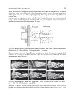
a) during test preparations b) “as-tested” FEM
Fig. 1. MD-500 helicopter model.
4. LS-DYNA model description
To predict the behavior of the MD-500 helicopter during a crash test, an LS-DYNA (Hallquist,
2006) finite element model (FEM) of the fuselage, as shown in Figure 1b, was developed and
reported in (Annett and Polanco, 2010). The element count for the fuselage was targeted to not
exceed 500,000 elements, including seats and occupants; with 320,000 used to represent the
energy absorbing honeycomb and skid gear. Shell elements were used to model the airframe
skins, ribs and stiffeners. Similarly, the lifting and pullback fixtures, and the platform
supporting the data acquisition system (mounted in the tail) were modeled using rigid shells.
Ballast used in the helicopter to represent the rotor, tail section, and the fuel was modelled as
concentrated masses. For materials, the fuselage section is modeled using Aluminum 2024-T3
with elastic-plastic properties, whereas the nose is fiberglass and the engine fairing is Kevlar
fabric. Instead of using the complete “as-tested” FEM model, this study uses a simplified model
created by removing the energy absorbing honeycomb, skid gears, anthropomorphic dummies,
data acquisition system, and lifting/pull-back fixtures. After these changes, the resulting
simplified model is shown in Figure 2. Even with all these components removed, the simplified
model had 27,000 elements comprised primarily of shell elements to represent airframe skins,
ribs and stiffeners. The analytical test case used for calibration, simulates a helicopter crash onto
a hard surface with vertical and horizontal speeds of 26 ft/sec and 40 ft/sec, respectively. For
illustration, Figure 3 shows four frames from an LS-DYNA simulation as the helicopter
impacts the hard surface.


Fig. 2. Simplified finite element model.

Multi-Dimensional Calibration of Impact Models
449
5. Example results

Results described here are derived from the simplified LS-DYNA model, as shown in Figure
2. This simplified model reduced the computational time from days to less than seven
minutes and allowed for timely debugging of the software and demonstration of the
methodology, which is the main focus of the chapter. Nonetheless, the same approach can
be applied to the complete “as-tested” FEM model without modifications.


Fig. 3. Four frames of the LS-DYNA simulation as the helicopter impacts the hard surface.
For evaluation purposes, simulated data are used in lieu of experimental data. Because
more often than not analytical model predictions do not agree with the measured data, the
simplified model was arbitrarily perturbed. Knowledge of the perturbations and areas
affected are not revealed until the entire calibration process is completed. Data from this
model, referred to as the perturbed model, takes the place of experimental data. In this
study, no test uncertainty is considered. Therefore, only 1 data set is used for test.


a) wireframe with 405 nodes b) sensor placement
Fig. 4. Helicopter wireframe for a) simplified model b) simulated test sensor placement and
numbering.
t = 0.036 sec
t = 0.00 sec
t = 0.018 sec t = 0.060 sec
y
z
x

Aeronautics and Astronautics
450
Figure 4(a) depicts a wireframe of the simplified model showing only 405 nodes.
Superimposed is a second wiring frame with connections to 34 nodes identified by an

optimal sensor placement algorithm. At each node there can be up to 3 translational
measurements, however, here the placement algorithm was instructed to place only 41
sensors. Figure 4(b) shows the location for the 41 sensors. Results from the optimal sensor
placement located 8 sensors along the x direction, 10 sensors along the y direction, and 23
sensors along the z direction.
5.1 Initial parameter selection
Calibration efforts begin by selecting model parameters thought to be uncertain. Selecting
these parameters is perhaps the most difficult step. Not knowing what had been changed in
the perturbed model, the initial study considered displacements, stress contours, and plastic
strain results at different locations on the structure before selecting the modulus of elasticity
and tangent modulus at various locations. The parameters and uncertainty ranges selected
are shown in Table 1. Without additional information about parameter uncertainty, the
upper and lower bounds were selected using engineering judgment with the understanding
that values anywhere between the bounds were equally likely.

No.
Parameter Description
Nominal LowerBound Upper Bound
1 E back panel (lbs/in
2
) 10,000,000 8,000,000 12,000,000
2 E subfloor ribs (lbs/in
2
) 10,000,000 8,000,000 12,000,000
3 E keel beam web (lbs/in
2
) 9,880,000 7,904,000 11,856,000
4 E stinger upper tail (lbs/in
2
) 10,000,000 8,000,000 12,000,000

5 E stinger lower tail (lbs/in
2
) 10,000,000 8,000,000 12,000,000
6 E
t
subfloor ribs (lbs/in
2
) 134,200 107,360 161,040
7 E
t
keel beam web (lbs/in
2
) 134,200 107,360 161,040
8 E
t
lower tail stinger (lbs/in
2
) 134,200 107,360 161,040
Table 1. Initial parameter set description
With the parameter uncertainty definition in Table 1, LS-DYNA models can be created and
executed to study the calibration metrics as described earlier. As an example, 150 LS-DYNA
runs with the simplified model were completed while varying parameters over the ranges
shown in Table 1. To construct the uncertainty bounds for each of the 150 runs,
(, )Qtp is
computed from velocities at 41 sensors (see Figure 4) and plotted in Figure 5 as a function of
time; analysis (dashed-blue) and the simulated test (solid-red). With this sample size, the
probability of being able to reconcile test with analysis during times when test results are
outside the analysis bounds is less than 1/150 (recall that the simulated test data is from the
perturbed model). Figure 5 shows that during the time interval between 0.01 and 0.02
seconds, the analysis bounds are above the test. Therefore, it is unlikely that one would be

able to find parameter values within the selected set to reconcile analysis with test. This
finding prompted another look at parameter selection and uncertainty models to determine
a more suitable set.
5.2 Revised parameter selection
A second search for a revised parameter set involved conversations with the model
developer and additional runs while varying parameter bounds to see their effect on
1
M
.

Multi-Dimensional Calibration of Impact Models
451
The second set of parameters selected, after considering several intermediate sets, consisted
of thicknesses at various locations in the structure. A concern with varying thickness is its
effect on structural mass. However, because 80% of the helicopter model is comprised of
non-structural masses, thickness changes had little impact on the total mass. Table 2 shows
a revised parameter set and ranges selected for the second study.
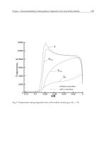
6. Evaluation of calibration metrics with revised parameter set
Results for metric
1
M
using the revised parameter set are shown in Figure 6; solid red is
()
e
Qtwith the simulated test data and in dotted blue lines are analysis bounds using 50 LS-
DYNA runs. With 50 runs, the probability that LS-DYNA would produce results outside
these bounds is less than 1/50. Consequently, if the test results are outside these bounds, the
probability of reconciling the model with test is also less than 1/50. Even though Figure 6
shows that, in certain areas, test results are very close to the analysis bounds; this new
parameter set provides enough freedom to proceed with the calibration process.

No.
Parameter
Description
Nominal
Lower
Bound
Upper
Bound
Calibrated
Value
1
Keel beam stiffener thickness
(in)
0.020 0.015 0.025 0.0161
2
Belly panel thickness (in) 0.090 0.08 0.135 0.1008
3
Keel beam thickness (in) 0.040 0.035 0.045 0.0358
4
Lower tail thickness (in) 0.040 0.035 0.045 0.0414
5 Back panel thickness (in) 0.020 0.015 0.025 0.0166
6 Upper tail thickness (in) 0.020 0.015 0.025 0.0168
Table 2. Revised parameter description


Fig. 5. Velocity vector 2-norm for analysis (with 150 LS-DYNA runs) and for simulated test.
0 0.01 0.02 0.03 0.04 0.05 0.06
1200
1400

1600
1800
2000
Time (sec)
Velocity 2-Norm


Test
Analysis
Analysis

Velocity
2-Norm
Time (sec)

Aeronautics and Astronautics
452


Fig. 6. Velocity vector 2-norm for analysis (with 50 LS-DYNA runs) and for simulated test.
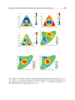
Thus far, in this study, metric M
1
has been used exclusively to evaluate parameter adequacy
and uncertainty bounds. What is missing from this evaluation is how well the model predicts
the response at all locations. Considering that impact shapes provide a spatial multi-
dimensional relationship among different locations, two models with similar impact shapes,
all else being equal, should exhibit similar responses at all sensor locations. With this in mind,
orthogonality results for the simplified model versus “test”, i.e., the perturbed model, are
shown in Figure 7. Essentially, the matrix M
2,

as defined in Eq. (4), is plotted with analysis



Fig. 7. Orthogonality results using impact shapes from the simulated test and baseline
model.
0 0.01 0.02 0.03 0.04 0.05 0.06
1200
1400
1600
1800
2000
Time (sec)
Velocity 2-Norm


Test
Analysis
Analysis


Velocity
2-Norm

Time (sec)
1 2 3 4 5 6 7 8 9 10
0.40
0.21
0.09
0.05

0.05
0.03
0.03
0.02
0.02
0.01
Test
Baseline


Final

Frequency (Hz)
0.39
0.18
0.08
0.07
0.05
0.04
0.03
0.03
0.02
0.02


0.1
0.2
0.3
0.4
0.5

0.6
0.7
0.8
0.9
Analysis

Simulated Test
Impact Shape Number

Multi-Dimensional Calibration of Impact Models
453
along the ordinate and test along the abscissa. Colors represent the numerical value of the
vector projections, e.g. a value of 1 (black) indicates perfect matching between test and
analysis. Listed on the labels are the corresponding shape contribution to the response for both
analysis (ordinate) and simulated test (top axis). For example, the first impact shape for
analysis (bottom left) contributes 0.4 of the total response as compared to 0.39 for test. It is
apparent that initial impact shape matching is poor at best with the exception of the first two
shapes. An example of an impact shape is provided in Figure 8. Here, a sequence of 8 frames
for the test impact shape number 2 (contribution
2
0.18


) expanded to 405 nodes, is shown.
Motion of the tail and floor section of the helicopter dominates.


Fig. 8. Test impact shape number 2 (
2
0.18


 ) animation sequence.
6.1.1 Sensitivity with revised parameter set
Another important aspect of the calibration process is in understanding how parameter
variations affect the norm metric
(, )Qtp . This information is used as the basis to remove or
retain parameters during the calibration process. As mentioned earlier, sensitivity results in
this study look at the ratio of the single parameter variance to the total variance of
(, )Qtp .
This ratio is plotted in Figure 9 for each of the six parameters considered (as defined in Table
2). Along the abscissa is time in seconds and the ordinate shows contribution to variance.
Colors are used to denote individual parameter contribution; total sum should approach 1
when no parameter interaction exists. In addition,
(, )Qtp
is shown across the top, for
reference. Because only 50 LS-DYNA runs are executed, an ERBF surrogate model is used to
estimate responses with 1000 parameter sets for variance estimates. From results in Figure
9, note that parameter contributions vary significantly over time but for simulation times
greater than 0.04 sec the upper tail thickness clearly dominates.
1
2
3
4
5
6
7
8