Electric Vehicles Modelling and Simulations Part 13 pdf

Minimization of the Copper Losses in
Electrical Vehicle Using Doubly Fed Induction Motor Vector Controlled

349










*
rs
m
r
L
s
L
PM
e
C
(4)
The copper losses are giving as:

2
r
i.
r

R
2
s
i.
s
R
cl
P

(5)
The motion equation is:


dt
d
Jd
e
C


(6)

In DFIM operations, the stator and rotor mmf’s (magneto motive forces) rotations are
directly imposed by the two external voltage source frequencies. Hence, the rotor speed
becomes depending toward the linear combination of theses frequencies, and it will be
constant if they are too constants for any load torque, given of course in the machine
stability domain. In DFIM modes, the synchronization between both mmf’s is mainly
required in order to guarantee machine stability. This is the similar situation of the
synchronous machine stability problem where without the recourse to the strict control of
the DFIM mmf’s relative position, the machine instability risk or brake down mode become

imminent.
3. Nonlinear vector control strategy
3.1 Double flux orientation
It consists in orienting, at the same time, stator flux and rotor flux. Thus, it results the
constraints given below by (7). Rotor flux is oriented on the d-axis, and the stator flux is
oriented on the q-axis. Conventionally, the d-axis remains reserved to magnetizing axis and
q-axis to torque axis, so we can write (Drid et al., 2005a, 2005b)










0
rq
sd
r
rd
ssq
(7)

Using (7), the developed torque given by (4) can be rewritten as follows:

.
rsc
k

e
C



(8)
where,
r
L
s
L
PM
c
k



s
 Appears as the input command of the active power or simply of the developed torque,
while
r
 appears as the input command of the reactive power or simply the main
magnetizing machine system acting.

Electric Vehicles – Modelling and Simulations

350
3.2 Vector control by Lyapunov feedback linearization
Separating the real and the imaginary part of (3), we can write:






















rq
u
4
f
dt
rq
d
rd
u

3
f
dt
rd
d
sq
u
2
f
dt
sq
d
sd
u
1
f
dt
sd
d
(9)
Where f
1
, f
2
, f
3
and f
4
are done as follows :














rd
rrq4sq34
f
rqr
rd
4
sd
33
f
sd
srq2sq12
f
sqs
rd
2
sd
11

f
(10)
With:

s
T
1
1

 ;
r
L
s
T
M
2

 ;
s
L
r
T
M
3

 ;
r
T
1
4



Tacking into account of the constraints given by (7), one can formulate the Lyapunov
function as follows

0
2
)
r
rd
(
2
1
2
)
ssq
(
2
1
2
rq
2
1
2
sd
2
1
V 
(11)
From (11), the first and second quadrate terms concern the fluxes orientation process

defined in (7) with the third and fourth terms characterizing the fluxes feedback control.
Where its derivative function becomes

)
r
rd
)(
r
rd
(
)
ssq
)(
ssq
(
rqrq
sdsd
V




(12)
Substituting (9) in (12), it results

)
r
rd
u
3

f()
r
rd
(
)
ssq
u
2
f()
ssq
(
)
rq
u
4
f(
rq
)
sd
u
1
f(
sd
V







(13)
Let us define the following law control as (Khalil, 1996):
Minimization of the Copper Losses in
Electrical Vehicle Using Doubly Fed Induction Motor Vector Controlled

351

















)
r
rd
(
4
K
r3

f
rd
u
)
ssq
(
3
K
s2
f
sq
u
rq2
K
4
f
rq
u
sd
1
K
1
f
sd
u


(14)
Hence (14) replaced in (13) gives:

0
2
)
r
rd
(
4
K
2
)
ssq
(
3
K
2
rq2
K
2
sd
1
KV



(15)
The function (15) is negative one. Furthermore, (14) introduced into (9) leads to a stable
convergence process if the gains K
i
(i=1, 2,3, 4) are evidently all positive, otherwise:
























0
t
)
*
ssq
lim(
0

t
)
*
r
rd
lim(
0
t
rq
lim
0
t
sd
lim
(16)
In (16), the first and second equations concern the double flux orientation constraints applied
for DFIM-model which are define above by (7), while the third and fourth equations define the
errors after the feedback fluxes control. This latter offers the possibility to control the main
machine magnetizing on the d-axis by 
rd
and the developed torque on the q-axis by 
sq
.
3.3 Robust feedback Lyapunov linearization control
In practice, the nonlinear functions fi involved in the state space model (9) are strongly
affected by the conventional effect of induction motor (IM) such as temperature, saturation
and skin effect in addition of the different nonlinearities related to harmonic pollution due
to the supplying converters and to the noise measurements. Since the control law developed
in the precedent section is based on the exact knowledge of these functions
fi, one can expect

that in real situation the control law (14) can fail to ensure flux orientation. In this section,
our objective is to determine a new vector control law making it possible to maintain double
flux orientation in presence of physical parameter variations and measurement noises.
Globally we can write:

i
f
i
f
ˆ
i
f 
(17)
On,
i
f
ˆ
: True nonlinear feedback function (NLFF)
i
f
: Effective NLFF
i
f
: NLFF variation around
i
f
.
Where:
i = 1, 2, 3 and 4.

Electric Vehicles – Modelling and Simulations

352
The ∆f
i
can be generated from the whole parameters and variables variations as indicated
above. We assume that all the ∆f
i
are bounded as follows: |∆f
i
| < 
i
; where are known
bounds. The knowledge of 
i
is not difficult since, one can use sufficiently large number to
satisfy the constraint|∆f
i
| < 
i
.
The ∆f
i
can be generated from the whole parameters and variables variations as indicated
above.
Replacing (17) in (9), we obtain
























rq
u
4
f
4
f
ˆ
dt
rq
d
rd

u
3
f
3
f
ˆ
dt
rd
d
sq
u
2
f
2
f
ˆ
dt
sq
d
sd
u
1
f
1
f
ˆ
dt
sd
d
(18)

The following result can be stated.
Proposition: Consider the realistic all fluxes state model (18). Then, the double fluxes
orientation constraints (7) are fulfilled provided that the following control laws are used

















)
r
rd
sgn(
44
K)
r
rd
(

4
K
r3
f
ˆ
rd
u
)
ssq
sgn(
33
K)
ssq
(
3
K
s2
f
ˆ
sq
u
)
rq
sgn(
22
K
rq2
K
4
f

ˆ
rq
u
)
sd
sgn(
11
K
sd
1
K
1
f
ˆ
sd
u


(19)

where K
ii
 
i
and K
ii
> 0 for i=1; 4.
Proof. Let the Lyapunov function related to the fluxes dynamics (18) defined by

0
2
)
r
rd
(
2
1
2
)
ssq
(
2
1
2
rq
2
1
2
sd
2
1
1
V 
(20)

One has








0V)
rd
sgn(
44
K
4
f)
r
rd
()
sq
sgn(
33
K
3
f)
ssq
(
)
rq
sgn(
22
K
2
f
rq

)
sd
sgn(
11
K
1
f
sd
1
V




(21)

where V

is given by (15). Hence the
i
f
variations can be absorbed if we take:
Minimization of the Copper Losses in
Electrical Vehicle Using Doubly Fed Induction Motor Vector Controlled

353


4
f

44
K
3
f
33
K
2
f
22
K
1
f
11
K




4
f
44
K
3
f
33
K
2
f
22
K

1
f
11
K




(22)

The latter inequalities are satisfied since
i
K >0 and
ii
K
ii
f 
Finally, we can write:


0V
1
V 

(23)

Hence, using the Lyapunov theorem (Khalil, 1996), on conclude that


























0
t
)
*
ssq
lim(
0
t

)
*
r
rd
lim(
0
t
rq
lim
0
t
sd
lim
(24)

The design of these robust controllers, resulting from (19), is given in the followed figure 2
The
indices w can be : sd, sq, rd and rq, (i = 1,2,3 and 4 )
4. Energy optimization strategy
In this section we will explain why and what is the optimization strategy used in this work.
Fig. 1 illustrates the problem which occurs in the proposed DFIM vector control system
when the machine magnetizing excitation is maintained at a constant level.
4.1 Why the energy optimization strategy?
Considering an iso-torque-curve (hyperbole form), drawn from (8) for a constant torque in
the
),(
rs
 plan and lower load machine ( Fig.1), on which we define two points A and B,
respectively, corresponding to the two machine magnetizing extreme levels. Theses points
concern respectively an excited machine (

ConstWb1
r



) and an under excited machine
(
ConstWb1.0
r

). Both points define the steady state operation machine or equilibrium
points. The machine rotates to satisfy the required reference speed acted by a given slope
speed acceleration
Const
dt
d



. So, the machine in both magnetizing cases must
develop a transient torque such as:

Electric Vehicles – Modelling and Simulations

354

0 1 2 3 4 5 6
-0.1
0
0.1

0.2
0.3
0.4
0.5
0.6
0.7
0.8
0.9
1
1.1

s
(wb)

r
(wb)
Transient
torque curve:

ro
C
dt
d
J 

Steady state torque curve:
ro
C
A A’
BB’

Fig. 1. Illustration of the posed problem in the DFIM control system with constant excitation.



 J
ro
C
dt
d
J
0r
C
eT
C
(25)
On the same graph, we define a second iso-torque-curve C
eT
=Const in the ),(
rs


plan. This
curve is a transient one on which we place two transient points
A’ and B’. Here we distinguish
the first transitions
A–A’ and B–B’ due to the acceleration set, respectively for each
magnetizing case. Both transitions are rapidly occurring in respect to the adopted control.
Once the machine speed reaches its reference, the inertial torque is cancelled ( = 0), then
the developed torque must return immediately to the initial load torque C

ro
, characterized
by the second transitions
A’–A and B’–B towards the preceding equilibrium points A and
B. One can notice that during the transition B–B’, corresponding to the under excited
machine, the stator flux can attain very high values greater than the tolerable limit (
maxs
 ),
and can tend to infinite values if the load torque C
ro
tends to zero. So the armature currents
expressed by the following formula deduced from (2) and (7) are strongly increased and can
certainly destruct the machine and their supplied converters.

s
.j
r
.
r
i
s
.j
r
.
s
i


(26)
Where,

r
L.
1
;
s
L.
1
;
r
L.
s
L.
M






In the other hand, for the case
A (excited machine), if the A–A’ transition remains tolerable,
the armature currents can present prohibitory magnitude in the steady state operation due
to the orthogonal contribution of stator and rotor fluxes at the moment that the machine is
sufficiently excited. The steady state armature currents can be calculated by (26), where we
can note the amplification effect of the coefficients ,  and .
Minimization of the Copper Losses in
Electrical Vehicle Using Doubly Fed Induction Motor Vector Controlled

355
4.2 Torque optimization factor (TOF) design

In the previous sub-section, the problem is in the transient torque, especially when the
machine is low loaded. So it becomes very important to minimize the torque transition such
as (Drid, 2005b):

0
dt
e
dC

(27)
where,

r
d
r
e
C
s
d
s
e
C
e
dC 





 (28)

This condition should be realized respecting the stator flux constraint given by

maxss

(29)
In this way the rotor and stator fluxes, though orthogonal, their modulus will be related by
the so-called TOF strategy which will be designed from the resolution of the differential
equations (27-28) with constraint (29) as follows:








maxss
0
srrs

(30)
from (29) we can write

maxsrsrrs


(31)
thus,

r

r
maxs
s








(32)
the resolution of (32) leads to

r
lnC
maxs
s



 (33)
where C is an arbitrary integration constant, therefore

)C(
e
r
maxs
s





(34)

Since, the main torque input-command in motoring DFIM operation is related to the stator
flux, it becomes dependent on the speed rotor sign and thus we can write







0if
s
0if
s
)sgn(
ssq
(35)

Electric Vehicles – Modelling and Simulations

356
with (35), (34), the rotor flux may be rewritten as follows

)C(
e
r

maxs
sq




(36)

The resolution of (32) gives place to the arbitrary integration constant C from which the
TOF-relationship (36) can be easily tuned. This one can be adjusted by a judicious choice of
the integration constant, while figure 2 presents TOF effect on armature DFIM currents with
C-tuning. Note that this method offers the possibility to reduce substantially the magnitude
of the armature currents into the machine and we can notice an increase in energy saving.
Hence using TOF strategy, we can avoid the saturation effect and reduce the magnitude of
machine currents from which the DFIM efficiency could be clearly enhanced.


-1.6 -1.2 -0.8 -0.4 0 0.4 0.8 1.2 1.6
0
50
100
-1.6 -1.2 -0.8 -0.4 0 0.4 0.8 1.2 1.6
0
50
100

s
(wb)
I
s

(A)
I
r
(A)
C = 2.3
C = 2.8
C = 1.8
C = 1.3
C = 2.8
C = 1.3
C = 1.8
C = 2.3

Fig. 2. TOF effect on armature DFIM currents
4.3 Torque-copper losses optimization (TCLO) design
In many applications, it is required to optimize a given parameter and the derivative plays a
key role in the solution of such problems. Suppose the quantity to be minimized is given by
the function
)x(f , and x is our control parameter. We want to know how to choose x to make
)x(f as small as possible. Let’s pick some x
0
as the starting point in our search for the best x.
The goal is to find the relation between fluxes which can optimize the compromise between
torque and copper losses in steady state as well as in transient state, (i.e. for all {C
e
} find
(
s
,
r

) let min{P
cl
}) (Drid, 2008). From (5), (8) and (26), the torque and copper losses can be to
written as:








2
s2
a
2
r1
a
cl
P
s
.
r
.
c
k
e
C
(37)
Minimization of the Copper Losses in

Electrical Vehicle Using Doubly Fed Induction Motor Vector Controlled

357
with :
)
2
)
s
L.(
s
R
2
)
s
L.
r
L.(
2
M
r
R
(
2
a
)
2
)
s
L.
r

L.(
2
M
s
R
2
)
r
L.(
r
R
(
1
a









The figure 3 represents the layout of (37) for a constant level of torque and copper losses in
the (
s
, 
r
) plan. These curves present respectively a hyperbole for the iso-torque and ellipse
for iso-copper-losses. From (37) we can write:

0
2
el
C
2
a
cl
P
2
r
2
c
k
4
r
2
c
k
1
a 
(38)
To obtain a real and thus optimal solution, we must have:

0
2
el
C
2
a

2
c
k
1
a4
4
cl
P
4
c
k 
(39)
The equation (39) represents the energy balance in the DFIM for one working DFIM point as
shown in fig.3. Then, one can write:

2
c
k
2
el
C
2
a
1
a4
cl
P  (40)
This equation shows the optimal relation between the torque and the copper losses.

-0.8 -0.6 -0.4 -0.2

0 0.2 0.4 0.6 0.8
-0.8
-0.6
-0.4
-0.2
0
0.2
0.4
0.6
0.8


 0


= 0
r (wb)
s (wb)
iso-torque
iso-copper-losses
Optimal solution

Fig. 3. The iso–torque curves and the iso–losses curves in the plan (
s
, 
r
)

Electric Vehicles – Modelling and Simulations

358
4.4 Finding minimum Copper-losses values
The Rolle’s Theorem is the key result behind applications of the derivative to optimization
problems. The second derivative test is used to finding minimum point.
We can rewrite (37) as:















2
r
.
2
c
k
2
e
C
2

a
4
r
2
c
k
1
a
2
r
.
2
c
k
2
e
C
2
a
2
r1
a
cl
P
r
.
c
k
e
C

s
(41)
The computations of the first and second derivatives show that the critical point is given
by:

4
1
2
c
k
1
a
2
a
2
e
C
rc









(42)
For which:

0
1
a8
4
rc
.
2
c
k
2
e
C
2
a6
4
rc
2
c
k
1
a2
2
r
d
)
rc
(
cl
P
2

d






(43)
We can see that the second derivative is positive and conclude that the critical point is a
relative minimum.
5. Simulation
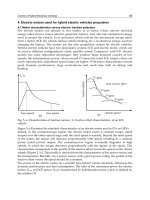
Figure 4 illustrates a general block diagram of the suggested DFIM control scheme. Here, we
can note the placement of optimization block, the first estimator-block which evaluates
torque and the second estimator-block which evaluates firstly the modulus and position
fluxes, respectively 
s
, 
r
, 
s
and


r
, from the measured currents using (2) and secondly the
feedback functions f
1
, f
2
, f

3
, f
4
given by (10). Optimization process allows adapting the main
flux magnetizing defined by rotor flux to the applied load torque characterized by the stator
flux. With the analogical switch we can select the type of the reference rotor flux. The switch
position 1, 2 gives respectively TCLO and TOF for optimized operation and the position 3
for a magnetizing constant level.
The Figure 5 shows the speed response versus time according to its desired profile drawn
on the same figure. Figure 6 illustrate the fluxes trajectory of the closed–loop system. It
moves along manifold toward the equilibrium point. We can notice the stability of the
system. Figures 7 and 8 show respectively the stator and the rotor input control voltages
versus time during the test. Figure 9 present the copper losses according to the stator flux
variations in steady state operation and we can see the contribution of the TCLO compared
to the TOF. Finally figure 10 present the dissipated energy versus time from which we can
observe clearly the influence of the three switch positions on the copper losses in transient
state. We can conclude that the TCLO is the best optimization.
Minimization of the Copper Losses in
Electrical Vehicle Using Doubly Fed Induction Motor Vector Controlled

359




~

*
rq
u

*
rd
u


*
réf


*
s


sq
sd

ˆ
,
ˆ

*
sd
u

*
sq
u

21

ˆ
,
ˆ
ff

Grid
DFIM

s
j
e



s


r

r
j
e


Inverter 1
Inverter 2
Stator Flux
controllers
Rotor Flux
controllers

Estimator

s
, 
r
, 
r
, 
s
, f
1
, f
2
, f
3
, f
4

43
ˆ
,
ˆ
ff

rq
rd

ˆ
,
ˆ

Speed
controller
Torque
Estimator
*
r


TCLO
TOF
1.1 wb
1
2
3
Switch
Grid


Fig. 4. General block diagram of control scheme




0 0.05 0.1 0.15 0.2 0.25 0.3 0.35 0.4
0
50
100
150
200

Time (sec.)
Speed (rd/s)


Fig. 5. Speed response

Electric Vehicles – Modelling and Simulations

360





-1.5 -1 -0.5
0 0.5 1 1.5
-1.5
-1
-0.5
0
0.5
1
1.5

r
(wb)


s
(wb)

Fig. 6. Fluxes trajectories of the closed–loop system





0 0.05 0.1 0.15 0.2 0.25 0.3 0.35 0.4
-400
-300
-200
-100
0
100
200
300
400
Time (sec.)
Stator voltage Vsa (v)



Fig. 7. The input control stator voltage response in the stator reference frames with TCLO
Minimization of the Copper Losses in
Electrical Vehicle Using Doubly Fed Induction Motor Vector Controlled

361

0 0.05 0.1 0.15 0.2 0.25 0.3 0.35 0.4
-400
-300
-200
-100
0
100
200
300
400
Time (sec.)
Rotor voltage Vra (v)


Fig. 8. The input control rotor voltage response in the stator reference frames with TCLO






)(wb
s

0.05 0.1 0.15 0.2 0.25 0.3 0.35
0

500
1000
1500
2000
Copper-Losses (W)


Fig. 9. Minimized copper losses in steady state operation with TOF and TCLO

Electric Vehicles – Modelling and Simulations

362
Time (sec.)
0 0.05 0.1 0.15 0.2 0.25 0.3 0.35 0.4
0
1
2
3
4
5
Dissipated energy (KJ)

Fig. 10. Total copper losses versus time during test for the three switch positions (Energy
saving illustration)
6. Conclusion
In this chapter was presented a vector control intended for doubly fed induction motor
(DFIM) mode. The use of the state-all-flux induction machine model with a flux orientation
constraint gives place to a simpler control model. The stability of the nonlinear feedback
control is proven using the Lyapunov function.
The simulation results of the suggested DFIM system control based on double flux

orientation which is achieved by the proposed DFIM control demonstrates clearly the
suitable obtained performances required by the references profiles defined above. The speed
tracks its desired reference without any effect of the load torque. Therefore the high control
performances can be well affirmed. To optimize the machine operation we chose to
minimize the copper losses. The proposed TCLO factor performs better than the already
designed TOF. Indeed, the energy saving process can be well achieved if the magnetizing
flux decreases in the same way as the load torque. It results in an interesting balance
between the core losses and the copper losses into the machine, so the machine efficiency
may be largely improved. The simulation results confirm largely the effectiveness of the
proposed DFIM control system.
7. Appendix
The machine parameters are:
Rs =1.2 ; Ls =0.158 H; Lr =0.156 H; Rr =1.8 ; M =0.15 H; P =2 ;J = 0.07 Kg.m² ; Pn = 4 Kw ;
220/380V ; 50Hz ; 1440tr/min ; 15/8.6 A ; cos = 0.85.
8. Nomenclature
s, r Rotor and stator indices.
d, q Direct and quadrate indices for orthogonal components
x Variable complex such as:




xm.jxex




.
Minimization of the Copper Losses in
Electrical Vehicle Using Doubly Fed Induction Motor Vector Controlled

363
x It can be a voltage as u , a current as i or a flux as 
*
x Complex conjugate
r
R,
s
R
Stator and rotor resistances
r
L,
s
L
Stator and rotor inductances
r
T,
s
T
Stator and rotor time-constants (T
s

r
=L
s, r
/R
s, r
)
 Leakage flux total coefficient (  =1- M²/L
r

L
s
)
M Mutual inductance
 Absolute rotor position
P
Number of pairs poles
 Torque angle

s
, 
r
Stator and rotor flux absolute positions
 Mechanical rotor frequency (rd/s)
 Rotor speed (rd/s)

s
Stator current frequency (rd/s)

r
Induced rotor current frequency (rd/s)
J

Inertia
d Unknown load torque
C
e
Electromagnetic torque
~ Symbol indicating measured value
^ Symbol indicating the estimated value

* Symbol indicating the command value
DFIM Doubly Fed Induction Machine
TOF Torque Optimization Factor
TCLO Torque Copper Losses Optimization
9. References
Vicatos, M.S. & Tegopoulos, J. A. (2003). A Doubly-Fed Induction Machine Differential
Drive Model for Automobiles,
IEEE Transactions on Energy Conversion, Vol.18, No.2,
(June 2003), pp. 225-230, ISSN 0885-8969
Akagi, H. & Sato, H. (1999). Control and Performance of a Flywheel Energy Storage System
Based on a Doubly-Fed Induction Generator-Motor,
Proceedings of the 30th IEEE
Power Electronics Specialists Conference, pp. 32-39, vol1, ISBN 0275-9306, Charleston,
USA, 27 June-1 July, 1999
Debiprasad, P. et al (2001). A Novel Control Strategy for the Rotor Side Control of a Doubly-
Fed Induction Machine.
IEEE Industry Applications Conference and Thirty-Sixth IAS
Annual Meeting, pp. 1695-1702, ISBN: 0-7803-7114-3, Chicago, USA, 30 September-
04 October 2001
Leonhard, W. (1997). Control Electrical Drives, Springier verlag, ISBN 3540418202, Berlin
Heidelberg, Germany
Wang, S. & Ding, Y. (1993). Stability Analysis of Field Oriented doubly Fed induction
Machine drive Based on Computed Simulation,
Electrical Machines and Power
Systems, Vol. 21, No. 1, (1993), pp. 11-24, ISSN 1532-5008
Morel, L. et al. (1998). Double-fed induction machine: converter optimisation and field
oriented control without position sensor,
IEE proceedings Electric power applications,
Vol. 145. No. 4, (July 1998), pp. 360-368, ISSN 1350-2352

Electric Vehicles – Modelling and Simulations

364
Hopfensperger, B. et al., (1999) Stator flux oriented control of a cascaded doubly fed
induction machine,
IEE proceedings Electric power applications, Vol. 146. No. 6,
(November 1999), pp. 597-605, ISSN 1350-2352
Hopfensperger, B. et al., (1999)
Stator flux oriented control of a cascaded doubly fed
induction machine with and without position encoder,
IEE proceedings Electric power
applications, Vol. 147. No. 4, (July1999), pp. 241-250, ISSN 1350-2352
Metwally, H.M.B. et al. (2002). Optimum performance characteristics of doubly fed
induction motors using field oriented control,
Energy conversion and Management,
Vol. 43, No. 1, (2002), pp. 3-13, ISSN 0196-8904
Hirofumi, A. & Hikaru, S. (2002). Control and Performance of a Doubly fed induction
Machine Intended for a Flywheel Energy Storage System,
IEEE Transactions on
Power Electronics, Vol. 17, No. 1, (January 2002), pp. 109-116, ISSN 0885-8993
Djurovic, M. et al. (1995). Double Fed Induction Generator with Two Pair of Poles,
IEE
Conferences of Electrical Machines and Drives, pp. 449-452, ISBN 0-85296-648-2,
Durham, UK, 11-13 September 1995
Leonhard, W. (1988). Adjustable-Speed AC Drives, Invited Paper,
Proceedings of the
IEEE, vol. 76, No. 4, (April 1988), pp.455-471. ISSN 0018-9219
Longya, X. & Wei C. (1995). Torque and Reactive Power control of a Doubly Fed Induction
Machine by Position Position Sensorless Scheme.
IEEE Transactions on Industry

Applications, Vol. 31, No. 3, (May/June 1995), pp 636-642 ISSN 0093-9994
Sergei, P., Andrea, T. & Tonielli, A. (2003). Indirect Stator Flux-Oriented Output Feedback
Control of a Doubly Fed Induction Machine,
IEEE Trans. On control Systems
Technology, Vol. 11, No. 6, (Nov. 2003), pp. 875–888, ISSN 1063-6536
Wang, D.H. & Cheng, K.W.E. (2004). General discussion on energy saving Power Electronics
Systems and Applications.
Proceedings of the First International Conference on Power
Electronics Systems and Applications, pp298-303, ISBN 962-367-434-1, USA, 9-11 Nov.
2004
Zang, L. & Hasan K.H, (1999). Neural Network Aided Energy Efficiency control for a Field
Orientation Induction Machine Drive.
Proceeding of Ninth International conference on
Electrical Machine and Drives, pp. 356-360, ISSN 0537-9989, Canterbury, UK, 1-3
September 1999
David, E. (1988). A Suggested Energy-Savings Evaluation Method for AC Adjustable-Speed
Drive Applications,”
IEEE Trans. on Industry Applications, Vol. 24, No. 6, (Nov/Dec.
1988), pp1107-1117, ISSN
0093-9994
Rodriguez, J. et al. (2002). Optimal Vector Control of Pumping and Ventilation Induction
Motor Drives.
IEEE Trans. on Electronics Industry, vol. 49, No. 4, (August 2002),
pp.889-895, ISSN
0278-0046
Drid, S., Nait_Said, M.S. & Tadjine, M. (2005). Double flux oriented control for the doubly
fed induction motor.
Electric Power Components & Systems Journal, Vol. 33, No.10,
(October 2005), pp. 1081-1095, ISSN 1532-5008
Drid, S., Tadjine, M. & Nait_Said, M.S. (2005). Nonlinear Feedback Control and Torque

Optimization of a Doubly Fed Induction Motor.
JEEEC Journal of Electrical Engineering
Elektrotechnický časopis, vol. 56, No. 3-4, (2005), pp. 57-63, ISSN 1335-3632
Drid, S.
, Nait-Said, M.S., Tadjine M. & Makouf A.(2008), Nonlinear Control of the Doubly
Fed Induction Motor with Copper Losses Minimization for Electrical Vehicle,
CISA08,
1st Mediterranean Conference on Intelligent Systems and Automation, AIP Conf.
Proc., Vol. 1019, pp.339-345, Annaba, Algeria, June 30-July 02, 2008
Khalil, H., (1996), Nonlinear systems. Prentice Hall, ISBN 0-13-067389-7, USA
16
Predictive Intelligent Battery Management
System to Enhance the Performance of
Electric Vehicle
Mohamad Abdul-Hak, Nizar Al-Holou and Utayba Mohammad
Electrical & Computer Engineering Department, University Of Detroit Mercy, Detroit,
USA
1. Introduction
The Electric Vehicle (EV) is emerging as state-of-the-art technology vehicle addressing
the continually pressing energy and environment concerns. The benefits of EV emerge
from these vehicles’ capability of sustaining their energy demands through electric grid
rather than fossil fuel consumption. Well- to-Wheel studies have shown that electric
drive (E-drive) offers the highest fuel efficiency and consequently the lowest emission of
green house gases. Grid electricity in the United States of America has been shown to be
four times cheaper than fuel given gasoline prices at $3/gallon. Consequently, it is
crucial to further optimize the electric-drive mode for EV. Battery capacity should be
designed to allow EV drivers reach their destination while avoiding unnecessary stops to
recharge their vehicles. However, this additional battery capacity would impact the
vehicle’s space, weight and cost. In view of these limitations, we propose integrating EVs
with the vision of Intelligent Transportation Systems (ITS). This chapter starts out by

putting the design of EVs into a broader perspective by proposing a Predictive
Intelligent Battery Management System (PIBMS), which will enhance the overall
performance of EVs including energy consumption and emissions using the ITS
infrastructure.
At the end of this chapter, the reader should have an understanding of the capabilities and
limitations of the PIBMS. It lays out the design foundation for the future implementation of
an interconnected EV equipped with PIBMS, which further contributes to the optimization
of energy efficiency and reduced emissions.
2. EV design challenges
Recent advancement in battery and charging technologies has allowed the Electric Vehicle
(EV) to be considered as the new generation of automotive transportation. However, the
physical dimensions, packaging environment and charging of EV batteries continues to be
the main challenge and the focus of attention in the development of EVs. Battery technology
selection continues to be the primary challenge in order to achieve the proper balance in the
EV design as illustrated in Figure 1 and described below.

Electric Vehicles – Modelling and Simulations

366

Fig. 1. EV Design Parameters
 Battery Capacity: EV battery capacity is predetermined by the battery design and cell
chemistry. Lithium polymer batteries are the target implementation for EV due mainly
to their high power-to-weight ratio.
 Vehicle Weight: EVs weight increases proportionally to battery capacity increase.
 Vehicle Space: Vehicle operators favor personal use of vehicle space. EV requires more
packaging space to house the battery in a safe environment. Generally, the battery is
packaged in the center of the vehicle where vehicle operators conventionally utilize this
space.
 Driving Range: EV can only run for 100-200 miles before recharging compared to

gasoline vehicle, which can drive more than 300 miles before refueling.
 Charging time: EV has no internal source for recharging the battery. EV charging time
ranges between 3-8 hours compared to 2-4 minutes of refueling for gasoline vehicle.
 Range Anxiety: EV operators are usually concerned with their vehicles’ limited driving
range, inadequate charging infrastructure, and long charging time.
 Energy Consumption: EV propulsion systems offer around 85% efficiency compared to
about 25 % efficiency for Internal Combustion Engines (ICE).
 Emission: EV emits no pollutants; however, power plant generating the EV electricity
may emit them.
While battery manufacturers are still pursuing further improvement in energy capacity, the
navigation technology and rapid advances in wireless communication technology can be
used to achieve the vehicle performance balance described as “Target” and presented in
Table 1.
Table 1 clearly shows the limitations for utilizing battery capacity as the only design variable
for achieving a balanced EV design that is acceptable for EV operators. To realize the success
of EVs, achieving the “Target” design option shall be exerted. This call for considering two
crucial aspects in addition to battery technology: Traffic information and wireless
communication.
The need to identify traffic conditions and the ability to transfer these conditions constitutes
the success of optimizing energy consumption and emission reduction in EVs.
Predictive Intelligent Battery Management
System to Enhance the Performance of Electric Vehicle

367
Realizing emission reduction in EVs is a crucial step toward emission free vehicles.
However, it requires a better understanding of emission free EVs and the ensuing energy
sources. These topics are addressed in the following section: EV Emission.


Table 1. EV System Design Option Evaluation

2. EV emission
2.1 Electrical energy source
An accurate assessment of EV emission requires the inclusion of the electrical energy source
associated emission with the generation and transmission. Electrical energy is generated
from two main sources as illustrated in Figure 2:
 Non-renewable source: Coal, natural gas, nuclear, petroleum
 Renewable source: wind, solar and geothermal
Non-renewable energy produces elevated Greenhouse Gas (GHG) emissions. Coal is
leading all other energy sources in terms of GHG emissions.
Renewable energy investment has to some extent been very limited due to the associated
high development cost. However government subsidiaries continue to make the renewable
energy investment more affordable.
The claim of EV proponents is that this type of vehicle is a Zero Emission Vehicle (ZEV).
This claim depends on many factors, but a key factor shall be highlighted. The EV operating
energy emission is a function of the energy source. The upstream Greenhouse gases (GHG)
emission is based on power plant types and efficiency. The claim of EV technology
proponents that this type of propulsion technology will offer a potential to reduce a long-

Electric Vehicles – Modelling and Simulations

368
term GHG emission can be verified with the implementation of the Well-To-Wheel (WTW)
emission model to analyze the GHG emission of the electrical energy source.


Fig. 2. Electrical Energy Source
2.2 EV configuration
The EV is mainly a conventional vehicle with the following main differences illustrated in
Figure 3 and listed below:
1. High voltage electric battery rather than a fuel tank to store and supply the required

operational energy
2. Electric motor rather than an internal combustion engine to propel the vehicle
3. Gear box rather than a transmission to couple the power from the electric motor to the
drive shaft
4. On Board or Off Board Charger to allow for recharging of the high voltage electric
battery
5. Direct current / Alternating current (DC/AC) inverter to convert the DC high voltage
battery into AC to drive the E-motor
6. DC/DC converter to convert the DC high voltage battery into DC low voltage battery
(Conventionally identified as 12 Volt battery)
2.3 EV efficiency
The EV overall efficiency can be classified in three main categories. The following section
describes the categories and their respective components:
2.3.1 Charging efficiency
Automotive charging standards are currently being developed worldwide to allow for DC
(Direct Current) charging. In contrast AC/DC (Alternating Current / Direct Current)
Predictive Intelligent Battery Management
System to Enhance the Performance of Electric Vehicle

369
charging standards have already been established and are currently being implemented in a
number of alternative vehicle technology production models such as the Chevy Volt, EV
SMART, Mitsubishi MIEV, Nissan Leaf and Tesla. DC charging enables the vehicle’s high
voltage DC battery to be directly charged from the charge station bypassing the vehicles’ on
board charger thus further improving charging efficiency and time. DC charging is the
target implementation for public charging enabling fast charge. Due to the associated high
cost of DC charging infrastructure, AC/DC charging will be the alternative and only
solution for residential charging.
The EV charging efficiency is the ratio of energy transferred to the high voltage battery to
the energy consumed from the AC source. Charging efficiency is highly dependent on

charging power and operating temperature. Figure 4 depicts a typical EV charging
efficiency operated at room temperature and utilizing an AC/DC onboard charger with a
maximum output power of 3500 W.


Fig. 3. Electric Vehicle Model


Fig. 4. EV Charging Energy Flow and Efficiency Diagram

Electric Vehicles – Modelling and Simulations

370
2.3.2 Operational efficiency
Generally the efficiency of the EV Electrical Motor (EM) is exceptionally high ~ 85 %
compared with an Internal Combustion Engine (ICE) ~ 25 %. Power losses in an EV are
negligible, in this section we will focus on power losses from key components occurring in
an electrical propulsion system during driving mode due to power conversion, operation
and propulsion. As illustrated in Figure 5 approximately 81.3 % of the energy stored in the
HV battery is utilized to propel the EV. Combining the EV overall charging efficiency with
the EV overall operational efficiency, the EV efficiency becomes ~ 67.9 % around four times
more efficient than an ICE propelled vehicle with an overall efficiency of ~ 14 %.


Fig. 5. EV Operating Energy Flow and Efficiency Diagram
2.3.3 Power source generation and transmission efficiency
For a full representation of energy and emission calculation, it is important to consider the
efficiency involved in energy recovery, processing and transportation. Complete vehicle
energy-cycle analysis tools, commonly known as Well-To-Wheel (WTW) analysis tools are
needed to provide an accurate assessment of EV overall efficiency and emission.

The U.S Environmental Protection Agency’s (EPA) offers an emission database “National
Emissions Inventory” (NEI); the database includes annual emissions associated with electric
energy generation.
To fully evaluate emission impact of EV, a Well-to-Wheel emission model shall be
considered such as the Greenhouse Gases, Regulated Emissions, and Energy Use in
Transportation (GREET). GREET was developed by the U.S. Department of Energy (U.S.
DOE) to allow researchers to evaluate emissions from a full fuel cycle for EVs and other
various propulsion technologies as depicted in Figure 6.
3. PIBMS architecture
Current EV architecture incorporates a Battery Management System (BMS) which is a
vehicle integrated electrical module responsible for monitoring State Of Charge (SOC) and
maintaining a suitable state of health (SOH) of the EV high voltage battery through
controlled charging and discharging processes of the battery cells.
Predictive Intelligent Battery Management
System to Enhance the Performance of Electric Vehicle

371

Fig. 6. WTW Emission Modeling
Adding a predictive and an intelligent component to the BMS design can make the
architecture of the EV more energy and emission efficient, as it would facilitate acquiring
traffic condition; offer a dynamic response to all future stochastic traffic flow situations
through travel route and drive profile advisement. The integration of the predictive and
intelligent components with the BMS led to the concept of the Predictive Intelligent Battery
Management System (PIBMS).
With the rapid advances in wireless communication, global positioning system and the
introduction of smartphones, the world is transitioning form being an online connected
world to become a mobile connected world. The PIBMS concept will be based on further
developing and integrating the existing technologies of the Global Positioning System
(GPS), the wireless communication technology “Dedicated Short Range communication”

(DSRC), and the advanced computing mobile phones identified as smartphone. The PIBMS
receives traffic information from traffic light controllers and roadside units, location data
from GPS and charge point data in the vicinity as depicted in Figure 7.
3.1 Intelligent Transportation System (ITS)
The technological progress in wireless communication, Global Positioning System (GPS)
and vehicle electronics is enabling the introduction of advanced technologies into the
transportation system commonly referred to as the Intelligent Transportation system (ITS).
3.1.1 Dedicated Short Range Communication (DSRC)
Dedicated Short Range Communication (DSRC) defined by the framework of the
international standards organization ASTM and standardized by the IEEE 802.11, IEEE
P1609.x and SAE J2735 standards, is a two-way short- to medium range (~1000 meters)
wireless communication designed for automotive application and currently being
systematically deployed throughout the U.S transportation system across the nation and
sponsored by the U.S Department of Transportation Research and Innovative Technology
Administration (RITA). DSRC enables the attainment of the following vehicle safety critical
components for vehicle communication:
 Fast Network Acquisition: To allow immediate establishment of communication
between vehicles and road side units
 Low Latency: To allow least execution time
 High Reliability: To allow high level of user reliability
DSRC offers the base and single wireless communication technology for future vehicular
safety communications; furthermore DSRC is gaining momentum among researchers for
future vehicular applications focused on energy optimization and emission reductions.

Electric Vehicles – Modelling and Simulations

372
DSRC
GPS
DGPS

Charge Point
Smart Phone
PIBMS
Traffic Light Controller
+ Road Side Unit

Fig. 7. PIBMS Communication Block Diagram
3.1.2 Positioning system
Real time vehicle position is required with a very high level of accuracy; this would allow
the system to optimize the output with both high confidence and reliability.
Several satellite receivers’ manufacturers offer systems with an extremely superior accuracy
such as the Topcon GR-3 receiver. The Topcon GR-3 is compatible with the US satellite
system GPS, the Russian satellite system GLONASS and the European satellite system
GALILEO. This receiver system claims a static accuracy of 3mm, a Real-Time Kinetic (RTK)
accuracy of 10 mm.
It is important to note than in cases where satellite navigation coverage is not available due
to for example driving through tunnels, Differential GPS data shall be used which would
offer in this case a slightly reduced accuracy.
3.2 PIBMS design
The PIBMS distinctive features are the predictive and the intelligent:
Predictive Intelligent Battery Management
System to Enhance the Performance of Electric Vehicle

373
 The predictive feature of the PIBMS is viable through the capability of the EV to
integrate the capability of vehicular wireless communication technology (DSRC) to
communicate traffic, charging infrastructure and vehicle data.
 The intelligent feature is offered through the application of a 2-scale dynamic
programming optimization approach onboard the PIBMS operated EV. The proposed
PIBMS architecture consists of six modules illustrated in Figure 8 and described

below:
1. Traffic Data Extractor (TDE): To extract the future traffic data from the ITS network
including traffic flow, intersection light status. This data is consequently used to
determine if alternative routes should be considered.
2. Vehicle Operation Mode (VOM): To provide the vehicle’s current operation modes
including vehicle speed, gear and SOC.
3. Trip Model Identifier (TMI): To learn the route road condition including slope and
distance, this is accomplished through the use of GPS data.
4. Trip Model Deflector (TMD): To re-route trip as found necessary following the
processing of future traffic data.
5. State Of Charge Optimizer (SOCO): To optimize battery energy the intelligent
algorithm found in this module is expected to have two key criteria: agile and dynamic.
6. Driver Feedback Control (DFC): To provide the driver feedback relative to drive style
including speed, acceleration, and deceleration.


Fig. 8. PIBMS Architecture