Supply Chain Management Pathways for Research and Practice Part 5 docx

Supply Chain Quality Management by Contract Design

69
5.2 Result comparison with other studies
In the following, we make a specific comparison with the result in Baiman et al. (2000, 2001),
which also involve the observability of the buyer’s inspection, the verifiability of external
failure, and the separability of the final product architecture separately.
When the manufacturer’s processing is observable and the external failure is verifiable,
Baiman et al. (2000) show that the first-best solution is achieved (Proposition 2a); however,
Table 1 shows that the first-best solution is achieved with extra contracts if the
manufacturer’s inspection is unobservable (Circumstances 5-7) or without extra contract if
the inspection is observable (Circumstances 13-15).
When the manufacturer’s processing is unobservable, the manufacturer’s inspection is
observable, and external failure is verifiable, Proposition 3 in Baiman et al. (2000) and
Proposition 4 in Baiman et al. (2001) show that the first-best solution is achieved; however,
Table 1 shows that the first-best solution is achieved without extra contract if the two parties
are not friends (Circumstances 9-16 in Not-Friends group) or if the two parties are friends
and the final product architecture is totally-separable (Circumstance 11 in Friends Group),
or with extra contract if the two parties are friends and the final product architecture is not-
totally-separable (Circumstances 9 and 10 in Friends group).
When the final product architecture is non-separable, Proposition in Baiman et al. (2001)
shows that the first-best solution cannot be achieved, but Table 1 shows that the first-best
solution can be attained without extra contract if the manufacturer’s inspection is observable
and with extra contract if the inspection is unobservable.
It is worthwhile to note that the above comparisons are just arguments by modeling
approaches to SCC. The results are based on different assumptions of the quality-based
supply chain.
6. Concluding remarks
Contract design for SCQM is discussed in a manufacturing supply chain. It is shown that
supplier and manufacturer in some circumstances must stipulate some items in contract to

guarantee coordination in SCQM, while other circumstances guarantee coordination
without extra contract. Furthermore, information system installation is an alternative
approach to coordination in those circumstances that need extra contracts to guarantee
coordination. The exact information system should be chosen based on characteristics of the
circumstances.
Two issues are highlighted in the manufacturing supply chain. The observability of the
buyer’s inspection is highlighted in supply chains such that the buyer further processes the
supplier’s product to be final product. The result is different from the case that the buyer
does not further process the supplier’s product. If the buyer’s inspection is unobservable,
the supplier will be exposed to moral hazard. Moreover, the extra conditions in which the
first-best solution is achieved are different from the ones in supply chains such that the
buyer does not process the supplier’s product further. In this chapter, the situation that the
manufacturer’s inspection is unobservable is corresponding with two extra conditions: (1)
the supplier is not responsible for the external failure caused by the manufacturer’s defect,
and (2) the supplier’s product price and the proportion of customer dissatisfaction the
supplier is responsible for satisfy
//(1)ds s



 .
The interactions between the external failure’s verifiability, the final product architecture’s
separability, and the two parties’ relationship are also highlighted. The three factors do not

Supply Chain Management – Pathways for Research and Practice

70
independently influence the contract design. Only if the external failure is verifiable, the
other two factors will be taken into account. The final product architecture’s separability and
the two parties’ relationship have the same hierarchy and have interactive influences. In this

chapter, an external failure-sharing mechanism is employed to connect the three factors.
7. Acknowledgment
This study was supported by the National Natural Science Foundation of China under
Grant No.70872091 and No.70672056.
8. Appendix
This Proof of Proposition 1: It is only to prove that the solution of maximization problem
coincides with the first-best solution if and only if the conditions are satisfied in the
circumstance.
The Lagrangian for the maximization problem in Circumstance 1 of Section 4 is
123
()
MS
MMMS S
qq
LP P P P P v


     with
1

,
2

,
3

and

as Lagrange multipliers
on constraints (B), (C), (D), and (E). The first-order conditions of the Lagrangian are

13
()() () ()() ()0
M
qS SMM S
LdqdmqMqMqmdmqd




         
, (A1)

23
[ (1 ) (1 )](1 ) ( ) ( ) [ (1 ) ][ ( )] 0
SS
LsdsqII qsd





   
, (A2)
1
23
()()( )( )[(1)(1)][ ( )]
[ (1 ) (1 )] ( ) { ( )[ (1 ) (1 )] ( )} 0
S
qMM
SMS

Ldqdmqsdmd
sd s Sq ds m q Sq
       
      
           
 
   
, (A3)

33
12
[( 1)(1 ) ](1 )(1 ) [( 1) ][1 (1 )]
(1 )(1 ) 0
SSM
SS
Lqs qmq
mq s q



      

(A4)

3312
[( 1)(1 ) ] (1 ) [( 1) ] (1 ) (1 ) 0
SSMSS
Lqs qmqmqsq



       . (A5)
Let
ˆ
ˆˆ ˆ
ˆ
{,,,,}
MS
qq


be the solution of the maximization problem.
On the one hand, if the first-best solution is achieved,
ˆ
S
q ,
ˆ
M
q and
ˆ

must satisfy (B0), (C0),
and (D0). Comparing (B), (C) with (B0), (C0), we have
()ds



 and ()0md


.

Since 0

 , then 0m

, 0 1s

 , and
//(1)ds s



.
On the other hand, the only thing we have to prove is that if 0m

, 0 1s, and
//(1)ds s

 then
123
,, 0


and 1


. Because if
123
,, 0



and 1

 exist
LPv and the first-best solution is derived. Firstly Plugging 0m

into (A1) and
comparing with (B) we have
1
0


since ()0
M
Mq



, and plugging //(1)ds s



 into
(A2) and comparing with (C), we have
2
0


since () 0I





. Secondly, plugging (D), (D0),
and
12
,0


 into (A3) we have
3
0


since ()0
S
Sq



. Finally, plugging 0m 
and
123
,, 0


into (A4) we have 1


since 0 1s


 . At this moment, (A3) is also
satisfied.

Supply Chain Quality Management by Contract Design

71
Proof of Proposition 2: The Lagrangian for the maximization problem in Circumstance 2 of
Subsection 4.1 is
23
()
S
MMS S
q
LP P P P v



 with
2

,
3

, and

as Lagrange
multipliers on constraints (C), (D), and (E). The first-order conditions of the Lagrangian are

3
()() ()() ()0

M
qS SM S
L d q d mq M q m d mq d



         , (A6)

23
[ (1 ) (1 )](1 ) ( ) ( ) [ (1 ) ][ ( )] 0
SS
LsdsqII qsd





   
, (A7)

2
3
( ) ( )( ) ( )[ (1 ) (1 )] [ (1 ) (1 )]
( ) { ( )[ (1 ) (1 )] ( )} 0,
S
qMM
SMS
Ldqdmqssds
Sq ds m q Sq
        


            
 

(A8)
332
[( 1)(1 ) ](1 )(1 ) [( 1) ][1 (1 )] (1 )(1 ) 0
SSMS
Lqs qmqsq


 
      (A9)

332
[( 1)(1 ) ] (1 ) [( 1) ] (1 ) (1 ) 0
SSMS
Lqs qmqsq


      
. (A10)
Let
ˆ
ˆˆ ˆ
ˆ
{,,,,}
MS
qq



be the solution of the maximization problem.
We only prove that if 0 1
s

 and //(1)ds s



 then
23
,0



and 1

 . Firstly,
plugging
//(1)ds s


 into (A7) and comparing with (C) we have
2
0


. Secondly,
plugging (D), (D0) and
2

0


into (A8) we have
3
0


. Finally, plugging
23
,0


into (A9) and (A10) we have
( 1)(1 )(1 )(1 ) ( 1) [1 (1 )] 0
SSM
qs qmq



 
and
(1)(1 )(1)(1)(1 )0
SSM
qs qm q


  . The two equations imply
( 1)[(1 )(1 ) ] 0
SS

qq

 
. Then 1


, since
01
S
q


and 1


.
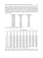
Proof of Corollary 1: The process of proof is tantamount to solve two maximization
problems

*
0,1;,0
(, ,,,)
S
M
SM
q
Maximize P q q




 
(A)
subject to

*
(, ,,,)0
M
SM
Pqq



, (C)

*
(, ,,,)0
S
S
qSM
Pqq


, (D)

*
(, ,,,)
S
SM
P
qq

v

 . (E)
According to the proof of Proposition 3, the solution of the above problem coincides with
the first-best solution.
Proof of Proposition 3: The Lagrangian for the maximization problem in Circumstance 3 is
13
()
MS
MMS S
qq
LP P P P v

    with
1

,
3

, and

as Lagrange multipliers on
constraints (B), (D), and (E). Let
ˆ
ˆˆ ˆ
ˆ
{,,,,}
MS
qq



be the solution of the maximization
problem. We only prove that if 0
m

then
23
,0


and 1


.
Following the similar steps we have that if 0
m

then
13
,0


. It leaves to prove that
1

 . From the first-order conditions of the Lagrangian we have

Supply Chain Management – Pathways for Research and Practice

72

( 1)[(1 )(1 )(1 ) ] 0
SS
Lqsq




 , (A11)

(1)(1 )(1)0
S
Lqs



 . (A12)
If 0
s  we have ( 1)[(1 )(1 ) ] 0
SS
qq



 from (A11), while if 1s

we have
(1)(1 )(1)0
S
Lq



   from (A12). Hence it holds that 1


.
Proof of Proposition 4: The Lagrangian for the maximization problem in Circumstance 4 is
3
()
S
MS S
q
LP P P v

   with
3

and

as Lagrange multipliers on constraints (D) and
(E). By following the similar track as in the proof of proposition 3 we are able to obtain
3
0


and 1

 .
9. References
Arshinder; Kanda, A. & Deshmukh, S. (2008). Supply chain coordination: Perspectives,
empirical studies and research directions.

International Journal of Production
Economics
, Vol.115, pp. 316-335
Baiman, S.; Fischer, P. & Rajan, M. (2000). Information, contracting, and quality costs.
Management Science, Vol.46, No.6, pp. 776-789
Baiman, S.; Fischer, P. & Rajan, M. (2001). Performance measurement and design in supply
chains.
Management Science, Vol.47, No.1, pp. 173-188
Balachandran, K. & Radhakrishnan, S. (2005). Quality implications of Warranties in a supply
chain.
Management Science, Vol.51, No.8, pp. 1266-1277
Bhattacharyya, S. & Lafontaine, F. (1995). Double-Sided Moral Hazard and the Nature of
Sharing Contracts.
The RAND Journal of Economics, Vol.26, No.4, pp. 761-781
Che, Y.K. & Hausch, D. (1999). Cooperative investments and the value of contracting: Coase
vs. Williamson.
American Economic Review, Vol.89, pp. 125-147
Chen, F. (2003). Information sharing and supply chain coordination.
Handbooks in OR & MS,
Vol.11, pp. 341-421.
Corbett, C.; Zhou, D. & Tang C. (2004). Designing supply contracts: contract type and
information asymmetry.
Management Science, Vol.50, No.4, pp. 550-559
Fawcett, S.; Ellram, L. & Ogden, J. (2006).
Upper Saddle Rive, PrenticeHall, NJ
Foster, S.T. (2005). Towards an understanding of supply chain quality management.
Journal
of Operations Management
, Vol.26, pp. 461-467
Fudenberg, D. & Tirole, J. (1991).

Game theory, The MIT Press
Heagy, C.D. (1991). Determining optimal quality costs by considering cost of lost sales.
Journal of Cost Management, Vol.4, No.3, pp. 64-72
Hwang, I.; Radhakrishnan, S. & Su, L. (2006). Vendor certification and appraisal:
implications for supplier quality.
Management Science, Vol.52, No.10, pp. 1472-1482
Ittner, C.; Nagar, V. & Rajan, M.V. (1999). An empirical analysis of the relevance of reported
quality costs.
Working paper, University of Pennsylvania, Philadelphia, PA
Kaynak, H. & Hartley, J. (2008). A replication and extension of quality management into the
supply chain.
Journal of Operations Management, Vol.26, pp. 468-489
Kim, J.; Lee, J.; Han, K. & Lee, M. (2002). Businesses as buildings: Metrics for the
architectural quality of internet businesses.
Information Systems Research, Vol.13,
No.3, pp. 239-254

Supply Chain Quality Management by Contract Design

73
Lee, H. (2004). The triple-A supply chain. Harvard Business Review, October(2004), pp. 102-
112
Lee, H.; Padmanabhan, V. & Whang, S. (1997). The bullwhip effect in supply chains.
Sloan
Management Review
, Vol.38, No.3, pp. 93-102
Li, X. & Wang, Q. (2007). Coordination mechanisms of supply chain systems.
European
Journal of Operational Research
, Vol.197, pp. 1-16

Liker, J.K. & Choi, T.Y. (2004). Building deep supplier relationships.
Harvard Business Review,
July(2004), pp. 104-113
Makis, V. & Jiang, X. (2003). Optimal replacement under partial observations.
Mathematics of
Operations Research
, Vol.28, No.2, pp. 382-394
Malchi, G. (2003). The cost of quality.
Contract Services Europe, May(2003), pp. 19-22
Maskin, E. & Tirole, J. (1999). Unforeseen contingencies and incomplete contracts.
Review of
Economic Studies
, Vol.66, pp. 83-144
Novak, S. & Eppinger, S. (2001). Sourcing by design: Product complexity and the supply
chain.
Management Science, Vol.47, No.1, pp. 189-204
Plambeck, E.L. & Taylor, T.A. (2006). Relationship in a dynamic production system with
unobservable behaviors and noncontractible output.
Management Science, Vol.52,
No.10, pp. 1509-1527
Rasmusen, E. (1989).
Games and Information. Blackwell Publisher.
Reyniers, D.J. & Tapiero, C.S. (1995a). The delivery and control of quality in spplier-
producer contracts.
Management Science, Vol.41, No.10, pp. 1581-1589
Reyniers, D.J. & Tapiero, C.S. (1995b). Contract design and the control of quality in a
conflictual environment.
European Journal of Operational Research, Vol.82, pp. 373-382
Robinson, C. & Malhotra, M. (2005). Defining the concept of supply chain quality
management and its relevance to academic and industrial practice.

International
Journal of Production Economics
, Vol.96, pp. 315-337
Saraf, N.; Langdon, C. & Gosain, S. (2007). IS application capabilities and relational value in
interfirm relationships.
Information System Research, Vol.18, No.3, pp. 320-339
Schweinsberg, C. (2009). In downturn, Chinese suppliers refocus on quality, reliability.
Ward’s Auto World, Vol.45, No.7, pp. 12
Sila, I.; Ebrahimpour, M. & Birkholz, C. (2006). Quality in supply chains: an empirical
analysis.
Supply Chain Management, Vol.11, No.6, pp. 491-502
Sosa, M.; Eppinger, S. & Rowles, C. (2004). The misalignment of product architecture and
organizational structure in complex.
Management Science, Vol.50, No.12, pp. 1674-
1689
Sower, V. (2004). Estimating external failure costs: A key difficulty in COQ systems.
Annual
Quality Congress Proceedings
, Vol.58, pp. 547-551
Swinney, R. & Netessine, S. (2009). Long-term contracts under the threat of supplier default.
Manufacturing & Service Operations Management, Vol.11, No.1, pp. 109-127
Tirole, J. (1999). Incomplete contracts: What do we stand?
Econometrica, Vol.67, No.4, pp.
741-781
Ulrich, K. (1995). The role of product architecture in the manufacturing firm.
Research Policy,
Vol.24, pp. 419-441
Sower, V. (2004). Estimating external failure costs: A key difficulty in COQ systems.
Annual
Quality Congress Proceedings

, Vol.58, pp. 547-551

Supply Chain Management – Pathways for Research and Practice

74
Wei, S.L. (2001). Producer-supplier contracts with incomplete information. Management
Science
, Vol.47, No.5, pp. 709-715
Yeung, A. (2008). Strategic supply management, quality initiatives, and organizational
performance.
Journal of Operations Management, Vol.26, pp. 490-502
6
Supply Chain Flexibility:
Managerial Implications
Dilek Önkal and Emel Aktas
Brunel Business School, Brunel University,
United Kingdom
1. Introduction
Today’s companies are forced into functioning in a challenging business world with
extensive uncertainties. Frontrunners turn out to be those companies that are able to foresee
the market swings and react swiftly with minimal adjustment costs and effective response
strategies. Hence, developing flexibility in adapting to sudden changes in global markets,
resource availabilities, and outbreaks of financial and political crises becomes an integral
part of effective management strategy. Supply chain management presents an especially
important domain where such flexibility is critical to achieving a consistently successful
performance.
Earlier research on flexibility in supply chains has focused primarily on manufacturing (e.g.,
Barad & Nof, 1997; De Toni & Tonchia, 1998; Gupta & Goyal, 1989; Kaighobadi &
Venkatesh, 1994; Koste & Malhotra, 1999; Mascarenhas, 1981; Parker & Wirth, 1999; Sethi &
Sethi, 1990). In contrast, recent studies have tended to examine a proliferation of different

dimensions like volume, launch, and target market flexibilities (Vickery, Calantone & Drőge,
1999); logistics flexibility potentially including flexibilities in postponement, routing,
delivery and trans-shipment (Barad & Sapir, 2003; Das & Nagendra, 1997); order quantity
and delivery lead time flexibilities (Wang, 2008); sourcing flexibility (Narasimhan & Das,
2000); launch flexibility and access flexibility (Sánchez and Pérez, 2005). Firm performance
has presented another core theme in recent work, with results pointing to the importance of
customer-supplier flexibility capabilities to improve competitiveness (Merschmann &
Thonemann, in press; Sánchez and Pérez, 2005). Duclos, Vokurka & Lummus (2003) argue
for the importance of organizational flexibility and information systems flexibility (in
addition to operations system, market, logistics, and supply flexibility) so that the supply
chains can function in a seamless succession of efficient processes; while More & Babu (2009)
claim that supply chain flexibility is a new strategic tool for management.
In thinking about the managerial implications of supply chain flexibility, it is useful to
distinguish among ‘flexible competencies’ (internal flexibility issues from the supplier
perspective) versus ‘flexible capabilities’ (customer perceptions on external flexibility issues)
(Zhang, Vonderembse & Lim, 2003). It is important in this regard to tease out the relevant
factors for suppliers and customers using procedures like Delphi (Lummus, Vokurka &
Duclos, 2005), where the different attributes could be identified and unified metrics could be
developed to enable communication across different perspectives (Gunasekaran, Patel &

Supply Chain Management – Pathways for Research and Practice

76
McGaughey, 2004). This is a complicated issue with performance measurement being a
multi-dimensional construct that needs to target operational parameters like efficiency in
addition to the stakeholder exposure factors like control and accountability (Parmigiani,
Klassen & Russo, 2011).
Supply chain risks and disruptions can be caused by natural disasters, unexpected
accidents, operational difficulties, terrorist incidents, and industrial or direct action. In any
case, supply chains need to be flexible enough to recover from any disruptions at the earliest

possible time. Moreover, it is possible to consider two different types of flexibility within the
supply chain context; volume/capacity flexibility that allows to decrease or increase
production according to the observed demand and delivery flexibility that allows to make
changes to the deliveries, e.g. adapting new delivery amounts or delivery dates. In line with
these ideas, Schutz and Tomasgard (2009) analyse volume, delivery, storage and operational
decision flexibilities in a supply chain under uncertain demand and arrive at a trade-off
between volume and delivery flexibility and operational decision and storage flexibility.
A recent survey on supply chain flexibility by More and Babu (2009) provides a
comprehensive definition of flexibility within the context of supply chain, summarizes the
methods used to model supply chain flexibility, and concludes with interesting future
research avenues. Although there is no general agreement on how to define supply chain
flexibility, the area has tremendous potential for researchers providing opportunities for
modelling and application of flexibility to the supply chain, interrelationships and trade-offs
between different types of flexibilities, industry-specific or business function-specific impact
of flexibility, and/or potential barriers to the implementation of flexibility.
In this chapter, we aim to focus on the synergies between supply chain flexibility and
forecasting, risk management, and decision making as the influential factors affecting
performance and management of supply chains. In light of the scarcity of studies
investigating supply chain flexibility and the pressing need for future work in this area, we
aim to (1) provide a review of extant literature, (2) highlight emerging research directions,
and (3) discuss managerial repercussions. In so doing, this chapter will emphasize three
areas that collectively play a critical role in determining the effectiveness of flexible supply
chains: forecasting, risk management, and decision making.
2. Forecasting and supply chain flexibility
Forecasts represent main inputs into planning and decision making processes in supply
chains. Predictions of future demands, resource requirements and consumer needs present
some areas where collaborative forecasting may play a significant role in contributing to
flexible supply chain performance. In fact, the quality of decisions and the resulting
outcomes may be argued to depend on the extent of information sharing and forecast
communication in flexible supply chains.

Planning and decision making processes in supply chains heavily rely on forecasts.
Accordingly, forecasting accuracy is a core factor that influences the performance of a
supply chain (Zhao, Xie & Leung, 2002). Bullwhip effect is a prime example of how
predictive inaccuracy can easily intensify through the supply chain (Chang & Lin, 2010),
crippling the affected partners. Predictions of future demands, resource requirements and
consumer needs present some areas where collaborative forecasting may play a significant
role in contributing to flexible supply chain performance.

Supply Chain Flexibility: Managerial Implications

77
While flexibility is argued to provide a way for eluding forecasting uncertainties (Bish,
Muriel & Biller, 2001), it may also be viewed as a means for benefitting from the
informational advantages and forecasting expertise of supply chain partners (Småros, 2003).
This may be especially critical given the strong influence of the organizational roles in
guiding the individual and group forecasts (Önkal, Lawrence & Sayım, 2011). Additionally,
biases such as overconfidence and optimism are found to have significant effects on supply
chain forecasts (Fildes et al, 2009), thus challenging predictive accuracy and synchronized
information flow among the decision makers. All these factors make collaborative
forecasting an indispensable tool for flexibility and responsive decision making in supply
chains (Caridi, Cigolini & de Marco, 2005; Derrouiche, Neubert & Bouras, 2008), as well as
for improving efficiency and competitiveness (Aviv, 2001; Helms, Ettkin &Chapman, 2000).
Supply chain flexibility requires extensive information and forecast sharing, and thus is
vulnerable to a variety of motivational factors that can potentially lead to significant
distortions (e.g., Mishra, Raghunathan & Yue, 2007). Various studies have clearly
demonstrated the impact of such forecasting errors and distortions on supply chain
performance (e.g., Zhao & Xie, 2002; Zhu, Mukhopadhyay &Yue, 2011). In this regard, the role
of trust in collaborative forecasting presents an extremely promising research area. Supply
chain relationships are acknowledged to rely on trust, with its role investigated mainly in the
context of information sharing and information quality (e.g., Chen, Yen, Rajkumar &

Tomochko, 2010). This can easily be extended to studies that focus on how trust among
partners could reduce individual and organizational biases (Oliva & Watson, 2009), leading to
forecast sharing and improved predictive accuracy for the whole supply chain.
In summary, collaborative forecasting and forecast sharing constitute vital areas for
enhanced decision making in flexible supply chains. Further research in this domain is likely
to face serious challenges emanating from behavioral factors and organizational dynamics,
but the rewards to flexible supply chain management will surely be worth the effort.
3. Risk management and supply chain flexibility
Uncertainties in the operating environment of firms reduce the reliability in terms of
delivering at the right time, at the right amount and quality. Uncertainty requires firms to
quickly respond to changing environments. Operating in a flexible supply chain helps the
firms to accomplish this rapid adaptation. On the other hand, increasing flexibility brings
along additional risks for the firms to undertake. Alignment, adaptability and agility
(flexibility) are fundamental elements for supply chain risk management. It is accepted that
flexibility increases supply chain resilience; however, firms are reluctant to invest in
flexibility when it is not clear how much flexibility is required. The higher the flexibility, the
riskier is the chain. However, there are some methods and models which help to mitigate
the level of risk associated with the level of flexibility. This section analyses the relationship
between supply chain flexibility and supply network risk management.
An interesting study focusing on risk management in a supply chain that is subject to
weather-related demand uncertainty is provided by Chen and Yano (2010). These
researchers focus on a manufacturer-retailer dyad of a seasonal product with weather
sensitive demand to examine weather-linked rebate for improving the expected profits. This
is an extension of rebate contracts which have several advantages over other contract types

Supply Chain Management – Pathways for Research and Practice

78
such as no required verification of leftover inventory and/or markdown amounts, and no
adverse effect on sales effort by the retailer. The paper reports interesting results on how the

weather-linked rebate can take many different forms, and how this flexibility allows the
supplier to design contracts that are Pareto improving and limit the reciprocal risks of
offering and accepting the contract. The structural results can be extended to allow the two
parties to limit their risk under the increased flexibility.
Table 1 lists a sample of relatively recent events that have affected the respective supply
chains which would have turned out having very different outcomes if the supply chains
had higher levels of flexibility and appropriate risk management practices.

Event Outcome Reference
September 1999: Taiwan
earthquake
Huge losses for many electronic firms that
use Taiwanese manufacturers as suppliers.
Sheffi, 2005

March 2000: Fire at the
Philips microchip plant
in Albuquerque, NM.
Nokia and Ericsson were affected. Nokia
resumed production in three days whereas
Ericsson shut down production with $400
million loss.
Latour, 2001
April – June 2003: SARS
outbreak
It is estimated that transportation industry
lost 38 billion RMB, wholesale and retail
trade industries lost 12 billion RMB and
manufacturing industry lost 27 billion RMB.
Ji and Zhu, 2008

Summer 2004: Below-
average temperature
decreased the demand
for certain products
Cadbury Schweppes’ drinks business was hit
by soggy summer weather.

Coca-Cola and Unilever pointed the weather
for low sales of soft drink and ice cream
products.

Nestle reported decreased demand for ice-
cream and bottled water due to poor weather.
Kleiderman,
2004
May 2008: earthquakes in
Sichuan, China
Severe damage to infrastructure network. Qiang and
Nagurney, 2010
March 2011: Japanese
earthquake
Large negative impact on the economy of
Japan and major disruptions to global and
local supply chains.
Nanto et al.,
2011
Table 1. Key events and outcomes underlining the importance of risk management in
supply chain
The list can easily be extended to include high profile events like natural disasters and
terrorism attacks in different regions. All these occurrences have dramatic effects on the

supply chains, whether these are humanitarian supply chains involving health aid or basic
food supply chains. Further research into embedding emergency flexibilities in these chains
via best case risk management practices will be extremely valuable for both the practitioners

Supply Chain Flexibility: Managerial Implications

79
and the academics aiming to improve supply chain management performance under
extremely demanding circumstances.
4. Decision making and supply chain flexibility
Existing literature defines supply chain flexibility as a reactive means to cope with uncertainty.
Networked companies in a dynamic and complex environment require coordination of their
multiple plants, suppliers, distribution centres, and retailers. There are numerous decision
making models (linear, non-linear, and multi-objective) which aim for coordination of the
supply network players and hence increase the overall flexibility of the chain.
Schutz and Tomasgard (2009) employ a stochastic programming model to balance supply
and demand in a supply chain from the Norwegian meat industry. The authors find that a
deterministic model of the supply chain produces as good results as does the stochastic
model given a certain level of flexibility in the chain. The level of extra capacity required to
obtain volume flexibility, number of products to achieve mix flexibility, or the level of
procurement flexibility stand as important decisions in the supply chain to improve market
responsiveness and resolve uncertainty-related problems. Das (2011) proposes a mixed
integer programming model for supply chain to address demand and supply uncertainty
along with market responsiveness. A scenario-based stochastic approach is utilized to model
the demand behaviour where they test the supply chain flexibility based on a pool of
suppliers. The proposed mixed integer programming model is tested to aid supply chain
managers in setting supplier flexibility, capacity flexibility, product flexibility and customer
service level flexibility.
On the other hand, Wadhwa and Saxena (2007) propose a decision knowledge sharing
model to improve collaboration in flexible supply chains. The main benefit of the model is to

facilitate sourcing and distribution decisions. Empirical results demonstrate that full
decision-sharing in a flexible supply chain leads to decreased total costs.
Given the abundance of decision models that may be employed to adopt or increase supply
chain flexibility, further work on comparative analysis of such models in different contexts
with systematic variations in levels of uncertainty appears to be highly promising.
5. Interconnectedness of forecasting, risk management and decision making
The three areas of analysis are not mutually exclusive. There is a definite need for studies to
focus on and explore the intersections of forecasting, risk management and decision making
in the context of supply chain flexibility. We will discuss these interactions next.
5.1 Decision making / risk management for supply chain flexibility
Risk management and decision making are inherently intertwined. Their interactions gain a
special significance for the plethora of managerial issues faced in efforts to introduce
flexibility to different aspects of supply chains. Yu et al. (2009) focuses on a two-stage
supply chain where the buying firm faces a non-stationary, price-sensitive demand of a
critical component and where two suppliers (primary and secondary) are available. The
authors suggest a mathematical model as a decision aid to choose the most profitable
sourcing strategies in the presence of supply chain disruption risks. It should be noted that

Supply Chain Management – Pathways for Research and Practice

80
the demand model used in this study is fairly simple and the supplier’s capacity is assumed
to be infinite. One critical limitation of this study is that it considers only the buyer’s profit
instead of examining the sourcing decisions from both parties’ point of view.
Giannikis and Louis (2001) develop a framework for designing a multi-agent decision
support system to aid the management of disruptions and mitigation of risks in
manufacturing supply chains. The agents responsible for communication, coordination, and
disruption management are built to simulate the supply chain which is occasionally subject
to abnormal events (e.g. an unusual fluctuation in the manufacturing process). Effective
disruptions management is assumed under collaborative behavior of supply chain partners

by learning from previous corrective actions for future decisions, suggesting risk mitigation
at operational and tactical levels. The most important result of this analysis may be that risk
management cannot be perceived as an individual process of each partner.
5.2 Forecasting / risk management for supply chain flexibility
Forecasts may be utilized as critical tools for risk management, and this gains a special
significance for managing flexible supply chains. Introducing successful mechanisms for
operational flexibilities throughout the supply chain requires effective integration of
forecasts into risk management strategies. This is a vital and yet challenging process for
supply chain management. Future work directed at exploring the role of forecasting – risk
management interactions for the performance of supply chains and their flexibility concerns
will prove especially useful in various contexts ranging from waste management to quality
control.
5.3 Forecasting / decision making for supply chain flexibility
As far as the uncertainty in demand and supply processes is concerned, flexibility improves
the performance of supply chains in terms of cost efficiencies and market response. The
close interplay between forecasting and decision making plays a vital role in managing such
uncertainties to expand the supply chain capabilities, resulting in enhanced system
performance throughout. Management of flexible supply chains necessitates planning for
alternative forecast scenarios and building efficient response strategies to tackle possibilities
of disruptions/crises/alterations for a variety of factors. Strong coordination mechanisms
among supply chain partners will be needed for information sharing, forecast
adjustment/synchronization, and group decision making.
6. Conclusion and directions for future research
Integrating flexibility into supply chains requires building efficient response mechanisms
for adapting to changes in a host of internal and external factors. In today’s competitive and
complex markets, supply chain management has to function along a dynamic interplay of
forecasting, risk management and decision making challenges (Wadhwa, Saxena & Chan,
2008). Developing effective supply chain strategies will need to involve a complicated
mixture of incentive alignment, information sharing, decision synchronization and
collaborative planning and forecasting (Cao & Zhang, 2011; Derrouiche, Neubert & Bouras,

2008; Simatupang & Sridharan, 2005). Enhancing information visibility (Wang and Wei,

Supply Chain Flexibility: Managerial Implications

81
2007), improving communication among supply chain partners, and developing effective
collaborative forecasting and decision support tools will prove immensely valuable in
attaining the desired strategic goals. The next decade of supply chain management research
may be expected to start providing answers to the multi-disciplinary challenges associated
with improving the global value and performance of flexible supply chains.
7. References
Aviv, Y. (2001), “The effect of collaborative forecasting on supply chain performance”,
Management Science, 47, 1326-1343.
Barad, M., and Nof, S., (1997), “CIM flexibility measures: A review and framework for
analysis and applicability assessment”, International Journal of Computer Integrated
Manufacturing, 10, 296-308.
Barad, M., and Sapir, D., (2003), “Flexibility in logistic systems-modeling and performance
evaluation”, International Journal of Production Economics, 85, 155-170.
Bish, E.K., Muriel, A., and Biller, S. (2001), “Managing flexible capacity in a make-to-order
environment”, Management Science, 51, 167-180.
Cao, M., and Zhang, Q. (2010), “Supply chain collaboration: Impact on collaborative
advantage and firm performance”, Journal of Operations Management, 29,
163-180.
Caridi,M., Cigolini, R. and de Marco, D. (2005), “Improving supply-chain collaboration by
linking intelligent agents to CPFR”, International Journal of Production Research, 43,
4191-4218.
Chang, P C., and Lin, Y K. (2010), “New challenges and opportunities in flexible and
robust supply chain forecasting systems “, International Journal of Production
Economics, 128, 453-456.
Chen, J.V., Yen, D.C., Rajkumar, T.M., and Tomochko, N.A. (2010), “The antecedent factors

on trust and commitment in supply chain relationships”, Computer Standards &
Interfaces, doi: 10.1016/j.csi.2010.05.003.
Chen, F.Y., Yano, C.A. (2010) Improving supply chain performance and managing
risk under weather-related demand uncertainty, Management Science, 56(8), 1380-
1397.
Das, K. (2011) Integrating effective flexibility measures into a strategic supply chain
planning model, European Journal of Operational Research, 211(1), 170-183.
Das, S., and Nagendra, P. (1997), “Selection of routes in a flexible manufacturing facility”,
International Journal of Production Economics, 85, 171-181.
Derrouiche, R., Neubert, G., and Bouras, A. (2008), “Supply chain management: A
framework to characterize the collaborative strategies”, International Journal of
Computer Integrated Manufacturing, 21, 426-439.
De Toni, A., and Tonchia, S. (1998), “Manufacturing flexibility: A literature review”,
International Journal of Production Research, 36, 1587-1617.
Derrouiche, R., Neubert, G., and Bouras, A. (2008), “Supply chain management: A
framework to characterize the collaborative strategies”, International Journal of
Computer Integrated Manufacturing, 21, 426-439.

Supply Chain Management – Pathways for Research and Practice

82
Duclos, L.K., Vokurka, R.J., and Lummus, R.R. (2003), “A conceptual model of supply chain
flexibility”, Industrial Management & Data Systems, 103, 446-456.
Fildes, R., Goodwin, P., Lawrence, M. and Nikolopoulos, K. (2009). “Effective forecasting
and judgmental adjustments: An empirical evaluation and strategies for
improvement in supply-chain planning”. International Journal of Forecasting, 25, 3-23.
Giannakis, M., Louis, M. (2011) A multi-agent based framework for supply chain risk
management, Journal of Purchasing and Supply Management, 17(1), 23-31.
Gunasekaran, A., Patel, C., and McGaughey, R.E. (2004), “A framework for supply chain
performance measurement”, International Journal of Production Economics, 2004, 333-

347.
Gupta, Y.P., and Goyal, S. (1989), “Flexibility of manufacturing systems: Concepts and
measurements”, European Journal of Operational Research, 43, 119-135.
Helms, M.M., Ettkin, L.P., and Chapman, S. (2000), “Supply chain forecasting: Collaborative
forecasting supports supply chain management”, Business Process Management, 6,
392-407.
Ji, G. and Zhu, C. (2008) Study on Supply Chain Disruption Risk Management Strategies
and Model, International Conference on Service Systems and Service Management, June
30 2008-July 2 2008, Melbourne, VIC.
Kaighobadi, M., and Venkatesh, K. (1994), “Flexible manufacturing systems: An overview”,
International Journal of Operations & Production Management, 14, 4, 26-49.
Kleiderman, A. (2004). Soggy summer spells boardroom gloom. BBC News (September 24),
date accessed: March 10, 2011.
Koste, L.L., and Malhotra, M.K. (1999), “A theoretical framework for analyzing the
dimensions of manufacturing flexibility”, Journal of Operations Management, 18, 75-
93.
Latour, A. (2001) Trial by fire: a blaze in Albuquerque sets off major crisis for cell-phone
giants, The Wall Street Journal; Eastern Edition, January 29.
Lummus, R.R., Vokurka, R.J., and Duclos, L.K. (2005), “Delphi study on supply chain
flexibility”, International Journal of Production Research, 43, 2687-2708.
Mascarenhas, B. (1981), “Planning for flexibility”, Long Range Planning, 14, 74–78.
Merschmann, U., and Thonemann, U.W. (in press), “Supply chain flexibility, uncertainty
and firm performance: An empirical analysis of German manufacturing firms”,
International Journal of Production Economics, doi:10.1016/j.ijpe.2010.10.013.
Mishra, B.K., Raghunathan, S., and Yue, X. (2007), “Information sharing in supply chains:
Incentives for information distortion”, IIE Transactions, 39, 863-877.
More, D., Subash Babu, A. (2009) Supply chain flexibility: a state-of-the-art survey,
International Journal of Services and Operations Management, 5(1), 29-65.
Nanto, D.K., Cooper, W.H., Donnelly, J.M., and Johnson, R. (2011) Japan’s 2011 Earthquake
and Tsunami: Economic Effects and Implications for the United States, CRS Report

for Congress, date accessed: May
10, 2011.
Narasimhan, R., and Das, A. (2000), “An empirical examination of sourcing’s role in
developing manufacturing flexibilities”, International Journal of Production Research,
38, 875-893.

Supply Chain Flexibility: Managerial Implications

83
Oliva, R., and Watson, N. (2009), “Managing functional biases in organizational forecasts: A
case study of consensus forecasting in supply chain planning”, Production and
Operations Management, 18, 138-151.
Önkal, D., Lawrence, M,. and Sayım, K. Z. (2011), “ Influence of differentiated roles on
group forecasting accuracy”, International Journal of Forecasting, 27, 50-68.
Parker, R.P., and Wirth, A. (1999), “Manufacturing flexibility: Measures and relationships”,
European Journal of Operational Research, 118, 429-449.
Parmigiani, A., Klassen, R.D., and Russo, M.V. (2011), “Efficiency meets accountability:
Performance implications of supply chain configuration, control, and capabilities”,
Journal of Operations Management, 29, 212-223.
Qiang, Q. and Nagurney, A., (2010) A Bi-Criteria Measure to Assess Supply Chain Network
Performance for Critical Needs Under Capacity and Demand Disruptions (January
15, 2010). Transportation Research, 2010. Available at SSRN:

Sánchez, A.M., and Pérez, M.P. (2005), “Supply chain flexibility and firm performance”,
International Journal of Operations & Production Management, 25, 681-700.
Schutz, P., Tomasgard, A., (2009) The impact of flexibility on operational supply chain
planning. International Journal of Production Economics, doi:10.1016/j.ijpe.2009.11.004
Sethi, A.K., and Sethi, S.P. (1990), “Flexibility in manufacturing: A survey”, International
Journal of Flexible Manufacturing Systems, 2, 289-328.
Sheffi Y. (2005) The resilient enterprise. Cambridge, MA: MIT Press.

Simatupang, T.M., and Sridharan, R. (2005), “An integrative framework for supply chain
collaboration”, International Journal of Logistics Management, 16, 257-274.
Småros, J. (2003), “Collaborative forecasting: A selection of practical approaches”,
International Journal of Logistics Research and Applications, 6, 245-258.
Vickery, S., Calantone, R., and Drőge, C. (1999), “Supply chain flexibility: An empirical
study”, The Journal of Supply Chain Management, Summer, 16-24.
Wadhwa, S., Saxena, A. (2007) Decision knowledge sharing: flexible supply chains in KM
context, Production Planning & Control, 18(5), 436-452.
Wang, E.T.G, and Wei, H L. (2007), “Interorganizational governance value creation:
Coordinating for information visibility and flexibility in supply chains”, Decision
Sciences, 38, 647-674.
Wang, Y C. (2008), “Evaluating flexibility on order quantity and delivery lead time for a
supply chain system”, International Journal of Systems Science, 39, 1193-1202.
Yu, H., Zeng, A.Z., Zhao, L. (2009). Single or dual sourcing: decision-making in the presence
of supply chain disruption risks. Omega, 37, 788-800.
Zhang, Q., Vonderembse, M.A., and Lim, J.S. (2003), “Manufacturing flexibility: Defining
and analyzing relationships among competence, capability and customer
satisfaction”, Journal of Operations Management, 21, 173-191.
Zhao, X., and Xie, J. (2002), “Forecasting errors and the value of information sharing in a
supply chain”, International Journal of Production Research, 40, 311-335.
Zhao, X., Xie, J., and Leung, J. (2002), “The impact of forecasting model selection on the
value of information sharing in a supply chain”, European Journal of Operational
Research, 142, 321-344.

Supply Chain Management – Pathways for Research and Practice

84
Zhu, X., Mukhopadhyay, S.K. and Yue, X. (2011), “Role of forecast errors on supply chain
profitability under various information sharing scenarios”, International Journal of
Production Economics, 129, 284-291.

Javier Pereira, Luciano Ahumada and Fernando Paredes
Faculty of Engineering, Universidad Diego Portales
Santiago de Chile
1. Introduction
One of the most relevant characteristics of inventory management methods is the
amplification phenomenon called the “bullwhip-effect”, defined as the upstream increasing
of production variability, caused by a supply chain’s demand variability at the retail level.
This effect has been extensively studied, both from industrial and theoretical points of view
(Takahashi et al., 1994). Among the multiple reasons mentioned in literature (Lee et al., 2000;
Takahashi et al., 1994; Warburton, 2004; Wu and Meixell, 1998), four features are frequently
reported at the origin of this phenomenon (Lee et al., 1997): demand signal processing,
strategic ordering behavior, ordering batching and price variations.
Geary et al. (2006) pointed out ten common causes of bullwhip-effect and the subsequent
re-engineering principles to eliminate or prevent amplification. Among them, the time
compression principle suggests that the most relevant principle to achieve this goal is the
existence of an optimal minimum lead time. Takahashi and Myreshka (2004) extensively
studied sources of bullwhip-effect and proposed several counter-measures for the demand,
ordering process and supply sides. Some of these counter-measures are: sharing information
about inventory and production levels among stages along the chain, controlling inventory
replenishment by a single method, reducing the lead-time, designing appropriate forecasting
methods (or eliminating forecasting practices) and implementing pull or hybrid methods.
It has been argued that the lack of flexibility in a supply chain is a consequence of
the bullwhip-effect. In order to analyze this argument, Pereira (1999) developed general
expressions for the amplification measure in the case of three ordering methods: push, pull
and hybrid. In a further contribution, Pereira and Paulre (2001) introduced the adjustment
degree of production to demand rate, a flexibility measure evaluating the distance between
the demand and production signals on each supply chain stage. Considering the ordering
methods above, an AR(1) demand process and a non-capacity-restricted supply chain model,
it was found that the adjustment degree behaves as a bullwhip-effect, especially in push
systems. More importantly, it was found that the bullwhip-effect is structurally due to

the upstream propagation of the demand forecasting. Chen et al. (2000) also studied the
increments of variability in a generic supply chain structure, for the specific case of a stationary
AR(1) process, finding that the demand forecasting importantly impacts the amplification
level in the supply chain. However, they did not explain how it is produced by forecasting
methods.

Bullwhip-Effect and Flexibility
in Supply Chain Management
7
2 Will-be-set-by-IN-TECH
In a recent work Pereira et al. (2009) have shown that for an AR(1) demand stochastic process,
flexibility on each stage of the supply chain strongly depends on the manager’s belief about
the downstream forecasting processes. Beliefs affect the decision rules in ordering methods,
structurally defining the adaptation capability in the supply chain. Then, flexibility could
be used as a strategy to keep amplification under control. In this chapter we present some
analytical results that explore this insight, considering the modeled supply chain and demand
process. Moreover, an introductory analysis of inventory amplification is presented, in order
to inspect the effect of manager’s belief on it. We propose that belief-based regulation may
improve the amplification levels both in production and inventory sides. But, it strongly
depends on the adopted forecasting method and the assumed demand process.
The remainder of this chapter is organized as follows. In section 2.1, the supply chain
model and ordering equations are presented. In section 2.2, the flexibility framework is
introduced and relevant preliminary results on adjustment degree for the modeled supply
chain are presented for push, pull and hybrid methods. In section 3, we introduce one of the
amplification acceptability criteria proposed in literature, which indicates the requirements
for control of the bullwhip effect. Further, the mathematical relation between the adjustment
degree and the amplification is presented, which allows us to express the amplification
acceptability criteria in terms of flexibility conditions. In section 3.3, a fading variable,
representing the manager’s belief on estimates, is analyzed in terms of its impact both on
production and inventory amplification measures. Conclusions are presented in section 4.

2. Preliminaries
2.1 The supply chain model
Consider a multi-echelon, single-item, supply chain composed by production stages P
i
(i =
1, . . . , n), stock sites B
i
(i = 0, . . . , n), and a supplier stage “Supplier", as shown in Fig. 1.
This will be called the reference model M (Pereira and Paulre, 2001).
Let us consider a periodic ordering method managing the production levels on each stage of
the supply chain (Takahashi and Myreshka, 2004). Then, the i-th production stage periodically
receives an order O
i
, which defines how many units of the item stocked in B
i
need to be
processed and further stocked in B
i−1
. The elapsed time between the instant when an order
is calculated and the moment where the ordered units are ready to be delivered (i.e., the lead
time) is considered an exogenous variable, identical in all stages: L
i
= L (i = 1, ,n).A
period is defined here as a unitary interval of time. Thus, t
∈ Z starts the t-th period; t + 1
starts the
(t + 1)-th, and so forth.











 










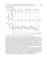
Fig. 1. Serial configuration of production stages
The following variables are defined in the model M:
Furthermore, the production rate at stage P
i
is given by
P
i
t
= O
i
t
−L

, (i = 1, . . . , n), (1)
which means that the manufacturing lead time between stages P
i
and P
1
can be written as
LT
(i)
= iL.
86
Supply Chain Management – Pathways for Research and Practice
Bullwhip-effect and Flexibility in Supply
Chain Management 3
D
t
: demand rate on stock site B
0
, during period t,
ˆ
D
i
t,t
+j
: t + j demand forecast, estimated at the end of t, for the stage P
i
,

ˆ
D
i

t
: marginal change of the sum of the demand forecast, calculated at the
end of t, for the stage P
i
,
O
i
t
: production order on the stage P
i
, calculated at the end of t,
P
i
t
: production rate on stage P
i
, during t, placed on stock B
i−1
at the
beginning of t
+ 1,
L
i
: lead time on stage i. We assume L
i
= L ∀i.
Inventory management systems differ in the way the production order on each stage is
defined. In the case of push, hybrid and pull management methods, the ordering equation
any stage i is expressed as (Pereira and Paulre, 2001):
Push : O

i
t
= D
t−(i−1)L
+
i
∑
j=1
Δ
ˆ
D
j
t
−(i−j)L
, (2)
Hybrid : O
i
t
= D
t−(i−1)L
+ Δ
ˆ
D
1
t
−(i−1)L
, (3)
Pull : O
i
t

= D
t−(i−1)L
. (4)
Notice that (3) characterizes a system where only the first stage operates in push.
2.2 Evaluating flexibility in the supply chain
A system is said flexible whenever it has the capability to self-adjust in response to changes in
its environment. The design of a flexible system implies control of three dimensions (Pereira
and Paulre, 2001): degree, effort and time of adjustment. More precisely, let a system and
its environment be characterized by the trajectories they take in the state spaces S and E ,
respectively. In addition, let us assume an observer is able to recognize the environment and
the system states e
t
∈ E and s
t
∈ S , at time t; she/he also identifies a logic L such that
L
(e
t−l
t
, s
t
)=(s
∗
t
, s
∗
t
− s
t
). (5)

This means that, given e
t−l
t
and s
t
, L allows the observer to define an expected state s
∗
t
∈ S
and its distance to the current state s
t
. Thus, the system responsiveness remains characterized
by l
t
≥ 0, indicating that the expected state depends on information provided to L in t, but
occurring in t
− l
t
. The considered system is said to be in partial equilibrium when L (e
t−l
t
, s
t
)=
(
s
∗
t
,0). Whenever s
∗

t
− s
t
 = 0, flexibility is the property that tends to realize the partial
equilibrium in the system. In order to do this, the system must expend a specific effort and
time. Thus, in given times t
1
, t
2
, ,t
n
, we assume that a flexible system dynamically adjusts
to demanded changes defined in a succesion of states D
= s
∗
1
, ,s
∗
n
.
Stage Push Hybrid Pull
i = 1 G G 0
i > 1 ϑ
i−1
+ H
i
ϑ
i−1
0
Table 1. Adjustment degree ϑ

i
for the three management methods
Now, we argue that the flexibility analysis provides a convenient framework to study the
supply chain bullwhip-effect. In fact, let us consider that D may be represented by the demand
process D
t
and the system states, on each stage, by P
t
. Then, given a stage i, a deviation
87
Bullwhip-Effect and Flexibility in Supply Chain Management
4 Will-be-set-by-IN-TECH
variable is defined as θ
i
t
= P
i
t
− D
t−iL
, which means that a demand signal received by the
stage i at time t
− (i + 1)L has a response at t − iL, i.e. within a leadtime L. This delay may
be considered the responsiveness capability (adjustment time) of this stage. The adjustment
degree on i is expressed as follows,
ϑ
i
=
V


θ
i
t

V
[
D
t−iL
]
∀
i ≥ 1, (6)
where V
[
·
]
denotes the variance of the argument. Notice that, as ϑ
i
decreases, the stage-i’s
adjustment of the production level to the delayed demand signal improves. Thus, the optimal
adjustment is reached when ϑ
i
= 0, ∀i.
It has been shown that, when the model M is considered, ϑ
i
, as measured for pull, push
and hybrid management methods, has the structure presented in Table 1 (Pereira and Paulre,
2001), where G and H
i
depend on the demand forecasting strategy (see section 3.2). This
result reveals that push-type stages propagate adjustment variability upstream in the supply

chain, scaling up or down the adjustment degree, in a very similar way to the bullwhip-effect
behavior.
3. Flexibility and amplification
3.1 The amplification of production
The bullwhip-effect in a supply chain is usually evaluated by an amplification measure, defined
as follows (Muramatsu et al., 1985),
Amp
i
=
V

P
i
t

V
[
D
t
]
. (7)
This metric may be interpreted as the scaling effect of demand variability, from the first to
upstream stages. It has been proposed that an adequate ordering method should satisfy
the following inequality (Muramatsu et al., 1985), called here the Muramatsu Amplification
Condition (MAC):
1
 Amp
1
 Amp
2

  Am p
n
. (8)
Hereinafter, let us see the relation between the amplification and the adjustment degree
measures. Indeed, expanding the expression for (6), it follows that
V

P
i
t
− D
t−iL

V
[
D
t
]
=
V

P
i
t

V
[
D
t
]

+
V
[
D
t−iL
]
V
[
D
t
]
−
2
V
[
D
t
]
cov

P
i
t
, D
t−iL

. (9)
Stationarity assumption allows us to write
ϑ
i

= Amp
i
+ 1 −
2
V
[
D
t
]
cov

P
i
t
, D
t−iL

. (10)
Defining γ
i
=
2
V
[
D
t
]
cov

P

i
t
, D
t−iL

, we have
Amp
i
= ϑ
i
+ γ
i
− 1. (11)
88
Supply Chain Management – Pathways for Research and Practice