Supply Chain Management Pathways for Research and Practice Part 7 pdf

A Fuzzy Goal Programming Approach for Collaborative Supply Chain Master Planning
109
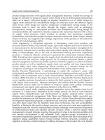
explore the influence of different weight structures on the results of the problem several
problem instances are generated. Solution results of the model obtained by Tiwari et al.
(1987) weighted additive approach are presented in Table 3. It is clear that determination of
the weights requires expert opinion so that they can reflect accurately the relations between
the different partners of a SC. In Table 3, w
1
, w
2
, w
3
and w
4
denotes the weights of
manufacturer’s, warehouses‘, logistic centres’ and shops‘ objectives for each instance. On the
other hand, Table 3 adds the degree of satisfaction of the objective functions for the
proposed method.

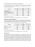
Objectives Upper bound Lower bound
COSTM 785545 543825
W
1
PROFIT 302078 171296
W
2
PROFIT 332787 198072
LC
1
COST 1359 1329

LC
2
COST 1187 1162
LC
3
COST 1227 1199
S
1
PROFIT 66552 64784
S
2
PROFIT 65825 64154
S
3
PROFIT 68787 67044
S
4
PROFIT 66448 64727
S
5
PROFIT 68486 66643
S
6
PROFIT 59838 58288
Table 2. Upper and lower bounds of the objectives.

Problem instances
1 2 3 4 5 6 7 8 9
w1
0.25 0.4 0.3 0.3 0.4 0.2 0.3 0.3 0.3

w2
0.25 0.2 0.2 0.2 0.1 0.2 0.4 0.2 0.1
w3
0.25 0.2 0.2 0.1 0.1 0.3 0.2 0.4 0.1
w4
0.25 0.2 0.3 0.4 0.4 0.3 0.1 0.1 0.5
µ
COSTM

0.7666 0.7707 0.7655 0.7655 0.9834 0.7672 0.7747 0.7760 0.9536
µ
W1PROFIT

1.0000 1.0000 1.0000 1.0000 0.9507 1.0000 1.0000 1.0000 0.9956
µ
W2PROFIT

0.5738 0.5670 0.5681 0.5681 0.1153 0.5738 0.5779 0.5780 0.1726
µ
LC1COST

0.0000 0.0000 0.0000 0.0000 0.0000 0.0000 0.4662 0.5629 0.0000
µ
LC2COST

1.0000 1.0000 0.0000 0.0000 0.0000 1.0000 1.0000 1.0000 0.0000
µ
LC3COST

0.0000 0.0000 0.0000 0.0000 0.0000 0.0000 1.0000 1.0000 0.0000

µ
S1PROFIT

0.8335 0.8335 1.0000 1.0000 1.0000 0.8335 0.4694 0.3224 1.0000
µ
S2PROFIT

0.6118 0.6118 0.9506 0.9506 0.9506 0.6118 0.6118 0.3830 0.9506
µ
S3PROFIT

0.9187 0.9187 1.0000 1.0000 1.0000 0.9187 0.5965 0.5965 1.0000
µ
S4PROFIT

0.9175 0.9175 1.0000 1.0000 1.0000 0.9175 0.5477 0.5477 1.0000
µ
S5PROFIT

0.8919 0.8919 1.0000 1.0000 1.0000 0.8919 0.4653 0.4653 1.0000
µ
S6PROFIT

0.8651 0.8651 1.0000 1.0000 1.0000 0.8651 0.5752 0.5752 1.0000
Table 3. Solution results obtained by Tiwari et al. (1987) approach.
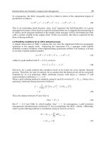
Table 4 shows the degree of satisfaction of each objective function obtained by Werners
(1988) approach with different values of the coefficient of compensation (). It is observed

Supply Chain Management – Pathways for Research and Practice
110

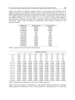
from Fig. 2 that the range of the achievement levels of the objectives increases with the
decrease of the coefficient of compensation, taking the maximum possible value in the
interval 0.5-0. That is, the higher the compensation coefficient γ values, the lower the
difference between the degrees of satisfaction of each partner of the decentralized SC. So, for
high values of γ, we can obtain compromise solutions for the all members of the SC, rather
than solutions that only satisfy the objectives of a small group of these partners. Table 4
shows in general terms, the reduction of the degree of satisfaction of logistics centres 1 and 3
and shop 2, at the expense of substantially increasing the degree of satisfaction of the logistic
center 2 and the rest of shops.Also, the degree of satisfaction related to warehouse 1
increases while reducing the degree of satisfaction associated to warehouse 2.


ϒ
0,9 0,8 0,7 0,6 0,5 0,4 0,3 0,2 0,1 0
µ
COSTM

0.7728 0.7722 0.7733 0.7723 0.7672 0.7672 0.7672 0.7672 0.7666 0.7672
µ
W1PROFIT

0.929 0.9262 0.9274 0.9317 1,0000 0.9762 0.9622 0.9622 1,0000 0.9622
µ
W2PROFIT

0.6405 0.6468 0.6442 0.6416 0.5736 0.5967 0.6099 0.6093 0.5732 0.6093
µ
LC1COST

0.6405 0.6405 0.6405 0.6405 0,0000 0,0000 0,0000 0,0000 0,0000 0,0000

µ
LC2COST

0.6405 0.6405 0.6405 0.6405 1,0000 1,0000 1,0000 1,0000 1,0000 1,0000
µ
LC3COST

0.6405 0.6405 0.6405 0.6405 0,0000 0,0000 0,0000 0,0000 0,0000 0,0000
µ
S1PROFIT

0.6405 0.6405 0.6405 0.6405 0.8335 0.8335 0.8335 0.8335 0.8335 0.8335
µ
S2PROFIT

0.6405 0.6405 0.6405 0.6405 0.6118 0.6118 0.6118 0.6118 0.6118 0.6118
µ
S3PROFIT

0.6405 0.6405 0.6405 0.6405 0.9187 0.9187 0.9187 0.9187 0.9187 0.9187
µ
S4PROFIT

0.6405 0.6405 0.6405 0.6405 0.9175 0.9175 0.9175 0.9175 0.9175 0.9175
µ
S5PROFIT

0.6405 0.6405 0.6405 0.6405 0.8919 0.8919 0.8919 0.8919 0.8919 0.8919
µ
S6PROFIT

0.6405 0.6405 0.6405 0.6405 0.8651 0.8651 0.8651 0.8651 0.8651 0.8651
Table 4. Solution results obtained by Werners (1988) approach.


Fig. 2. Range of the achievement levels of the objectives.
0,00
0,10
0,20
0,30
0,40
0,50
0,60
0,70
0,80
0,90
1,00
0.9 0.8 0.7 0.6 0.5 0.4 0.3 0.2 0.1 0
Achievement level
coefficient of compensation ()
max
min
range

A Fuzzy Goal Programming Approach for Collaborative Supply Chain Master Planning
111
7. Conclusion
In recent years, the CP in SC environments is acquiring an increasing interest. In general
terms, the CP implies a distributed decision-making process involving several decision-
makers that interact in order to reach a certain balance condition between their particular

objectives and those for the rest of the SC. This work deals with the collaborative supply
chain master planning problem in a ceramic tile SC and has proposes two FGP models for
the collaborative CSCMP problem based on the previous work of Alemany et al. (2010). FGP
allows incorporate into the models decision maker’s imprecise aspiration levels. Besides, to
explore the viability of different FGP approaches for the CSCMP problem in different SC
structures (i.e. centralized and decentralized) a real-world industrial problem with several
computational experiments has been provided. The numerical results show that
collaborative issues related to SC master planning problems can be considered in a feasible
manner by using fuzzy mathematical approaches.
The complex nature and dynamics of the relationships among the different actors in a SC
imply an important degree of uncertainty in SC planning decisions. In SC planning decision
processes, uncertainty is a main factor that may influence the effectiveness of the
configuration and coordination of SCs (Davis 1993; Minegishi and Thiel 2000; Jung et al.
2004), and tends to propagate up and down the SC, affecting performance considerably
(Bhatnagar and Sohal 2005). Future studies may consider uncertainty in parameters such as
demand, production capacity, selling prices, etc. using fuzzy modelling approaches.
Although the linear membership function has been proved to provide qualified solutions for
many applications (Liu & Sahinidis 1997), the main limitation of the proposed approaches is
the assumption of the linearity of the membership function to represent the decision maker’s
imprecise aspiration levels. This work assumes that the linear membership functions for
related imprecise numbers are reasonably given. In real-world situations, however, the
decision maker should generate suitable membership functions based on subjective
judgment and/or historical resources. Future studies may apply related non-linear
membership functions (exponential, hyperbolic, modified s-curve, etc.) to solve the CSCMP
problem. Besides, the resolution times of the FGP models may be quite long in large-scale
CSCMP problems. For this reason, future studies may apply the use of evolutionary
algorithms and metaheuristics to solve CSCMP problems more efficiently.
8. Acknowledgments
This work has been funded by the Spanish Ministry of Science and Technology project:
‘Production technology based on the feedback from production, transport and unload

planning and the redesign of warehouses decisions in the supply chain (Ref. DPI2010-
19977).
9. References
Alemany, M.M.E. et al., 2010. Mathematical programming model for centralised master
planning in ceramic tile supply chains. International Journal of Production Research,
48(17), 5053-5074.

Supply Chain Management – Pathways for Research and Practice
112
Barbarosoglu, G. & Özgür, D., 1999. Hierarchical design of an integrated production and 2-
echelon distribution system. European Journal of Operational Research, 118(3), 464-
484.
Bhatnagar, R. & Sohal, A.S., 2005. Supply chain competitiveness: measuring the impact of
location factors, uncertainty and manufacturing practices. Technovation, 25(5),443-
456.
Bellman, R.E. & Zadeh, L.A., 1970. Decision-Making in a Fuzzy Environment. Management
Science, 17(4), B141-B164.
Bilgen, B. & Ozkarahan, I., 2004. Strategic tactical and operational production-distribution
models: a review. International Journal of Technology Management, 28(2), 151-171.
Chen, M. & Wang, W., 1997. A linear programming model for integrated steel production
and distribution planning. International Journal of Operations & Production
Management, 17(6), 592 - 610.
Davis, T., 1993. Effective supply chain management. Sloan Management Review, 34, 35-46.
Dhaenens-Flipo, C. & Finke, G., 2001. An Integrated Model for an Industrial Production–
Distribution Problem. IIE Transactions, 33(9), 705-715.
Dudek, G. & Stadtler, H., 2005. Negotiation-based collaborative planning between supply
chains partners. European Journal of Operational Research, 163(3), 668-687.
Eksioglu, S.D., Edwin Romeijn, H. & Pardalos, P.M., 2006. Cross-facility management of
production and transportation planning problem. Computers & Operations Research,
33(11), 3231-3251.

Ekşioğlu, S.D., Ekşioğlu, B. & Romeijn, H.E., 2007. A Lagrangean heuristic for integrated
production and transportation planning problems in a dynamic, multi-item, two-
layer supply chain. IIE Transactions, 39(2), 191-201.
Erengüç, S.S., Simpson, N.C. & Vakharia, A.J., 1999. Integrated production/distribution
planning in supply chains: An invited review. European Journal of Operational
Research, 115(2), 219-236.
Fahimnia, B., Lee Luong & Marian, R., 2009. Optimization of a Two-Echelon Supply
Network Using Multi-objective Genetic Algorithms. In Proceedings of WRI World
Congress on Computer Science and Information Engineering, 2009, 406-413.
Hernández, J.E., Alemany, M.M.E., Lario, F.C. & Poler, R., 2009. SCAMM-CPA: A supply
chain agent-based modelling methodology that supports a collaborative planning
process. Innovar, 19(34), 99-120.
Jung, J.Y., Blau, G.E., Pekny, J.F., Reklaitis, G.V. and Eversdyk, D., 2004. A simulation based
optimization approach to supply chain management under demand uncertainty.
Computers & Chemical Engineering, 28(10), 2087-2106
Jung, H., Frank Chen, F. & Jeong, B., 2008. Decentralized supply chain planning framework
for third party logistics partnership. Computers & Industrial Engineering, 55(2), 348-
364.
Kallrath, J., 20
02. Combined strategic and operational planning – an MILP success story in
chemical industry. OR Spectrum, 24(3), 315-341.
Kumar, M., Vrat, P. & Shankar, R., 2004. A fuzzy goal programming approach for vendor
selection problem in a supply chain. Computers & Industrial Engineering, 46(1), 69-
85.

A Fuzzy Goal Programming Approach for Collaborative Supply Chain Master Planning
113
Lee, A.H.I., Kang, H Y. & Chang, C T., 2009. Fuzzy multiple goal programming applied to
TFT-LCD supplier selection by downstream manufacturers. Expert Systems with
Applications, 36(3, Part 2),.6318-6325.

Liang, T., 2006. Distribution planning decisions using interactive fuzzy multi-objective linear
programming. Fuzzy Sets and Systems, 157(10), 1303-1316.
Liang, T.F. & Cheng, H.W., 2009. Application of fuzzy sets to manufacturing/distribution
planning decisions with multi-product and multi-time period in supply chains.
Expert Systems with Applications, 36(2, Part 2), 3367-3377.
Liu, M.L. & Sahinidis, N.V., 1997. Process planning in a fuzzy environment. European Journal
of Operational Research, 100(1), 142-169.
Luh, P.B., Ni, M., Chen, H. & Thakur, L. S., 2003. Price-based approach for activity
coordination in a supply network. Robotics and Automation, IEEE Transactions on,
19(2), 335-346.
McDonald, C.M. & Karimi, I.A., 1997. Planning and Scheduling of Parallel Semicontinuous
Processes. 1. Production Planning. Industrial & Engineering Chemistry Research,
36(7), 2691-2700.
Mentzer, J.T., DeWitt, W., Keebler, J.S., Min, S., Nix, N.W., Smith, C.D. & Zacharia, Z.G.,
2001. Defining Supply Chain Management. Journal of Business Logistics, 22(2), 1-25.
Minegishi, S. & Thiel, D., 2000. System dynamics modeling and simulation of a particular
food supply chain. Simulation Practice and Theory, 8(5), 321-339.
Mula, J., Peidro, D., Díaz-Madroñero, M. & Vicens, E., 2010. Mathematical programming
models for supply chain production and transport planning. European Journal of
Operational Research, 204(3), 377-390.
Nie, L., Xu, X. & Zhan, D., 2006. Collaborative Planning in Supply Chains by Lagrangian
Relaxation and Genetic Algorithms. En Intelligent Control and Automation, 2006.
WCICA 2006. The Sixth World Congress on. Intelligent Control and Automation,
2006. WCICA 2006. The Sixth World Congress on. 7258-7262.
Ouhimmou, M., D’Amours, S., Beauregard, R., Ait-Kadi, D. & Singh Chauhan, S., 2008.
Furniture supply chain tactical planning optimization using a time decomposition
approach. European Journal of Operational Research, 189(3), 952-970.
Park, Y.B., 2005. An integrated approach for production and distribution planning in supply
chain management. International Journal of Production Research, 43(6), 1205-1224.
Peidro, D. & Vasant, P., 2009. Fuzzy Multi-Objective Transportation Planning with Modified

SCurve Membership Function. En Global Conference on Power Control and
Optimization. 101-110.
Selim, H., Araz, C. & Ozkarahan, I., 2008. Collaborative production-distribution planning in
supply chain: A fuzzy goal programming approach. Transportation Research Part E:
Logistics and Transportation Review, 44(3), 396-419.
Stadtler, H., 2009. A framework for collaborative planning and state-of-the-art. OR Spectrum,
31(1), 5-30.
Stadtler, H., 2005. Supply chain management and advanced planning basics, overview and
challenges. European Journal of Operational Research
, 163(3), 575-588.
Tanaka, H., Ichihashi, H. &
Asai, K., 1984. A formulation of fuzzy linear programming
problem bases on comparision of fuzzy numbers. Control and Cybernetics, 13, 185-
194.

Supply Chain Management – Pathways for Research and Practice
114
Timpe, C.H. & Kallrath, J., 2000. Optimal planning in large multi-site production networks.
European Journal of Operational Research, 126(2), 422-435.
Tiwari, R.N., Dharmar, S. & Rao, J.R., 1987. Fuzzy goal programming An additive model.
Fuzzy Sets and Systems, 24(1), 27-34.
Torabi, S.A. & Hassini, E., 2009. Multi-site production planning integrating procurement
and distribution plans in multi-echelon supply chains: an interactive fuzzy goal
programming approach. International Journal of Production Research, 47(19), 5475.
Vidal, C.J. & Goetschalckx, M., 1997. Strategic production-distribution models: A critical
review with emphasis on global supply chain models. European Journal of
Operational Research, 98(1), 1-18.
Walther, G., Schmid, E. & Spengler, T.S., 2008. Negotiation-based coordination in product
recovery networks. International Journal of Production Economics, 111(2), 334-350.
Werners, B., 1988. Aggregation models in mathematical programming. En Mathematical

Models for Decision Support. Springer, 295-305.
Zimmermann, H J., 1975. Description and optimization of fuzzy systems. International
Journal of General Systems, 2(1), 209.
Zimmermann, H.J., 1978. Fuzzy programming and linear programming with several
objective functions. Fuzzy Sets and Systems, 1(1), 45-46.
9
Information Sharing: a Quantitative Approach to
a Class of Integrated Supply Chain
Seyyed Mehdi Sahjadifar
1
, Rasoul Haji
2
,
Mostafa Hajiaghaei-Keshteli
3
and Amir Mahdi Hendi
4
1,3,4
Department of Industrial Engineering, University of Science and Culture, Tehran
2
Department of Industrial Engineering, Sharif University of Technology, Tehran
Iran
1. Introduction
The literature on the incorporating information on multi-echelon inventory systems is
relatively recent. Milgrom & Roberts (1990) identified the information as a substitute for
inventory systems from economical points of view. Lee & Whang (1998) discuss the use of
information sharing in supply chains in practice, relate it to academic research and outline
the challenges facing the area. Cheung & Lee (1998) examine the impact of information
availability in order coordination and allocation in a Vendor Managed Inventory (VMI)
environment. Cachon & Fisher (2000) consider an inventory system with one supplier and N

identical retailers. Inventories are monitored periodically and the supplier has information
about the inventory position of all the retailers. All locations follow an (R, nQ) ordering
policy with the supplier’s batch size being an integer multiple of that of the retailers. Cachon
and Fisher (2000) show how the supplier can use such information to allocate the stocks to
the retailers more efficiently.
Xiaobo and Minmin (2007) consider four different information sharing scenarios in a two-
stage supply chain composed of a supplier and a retailer. They analyse the system costs for
the various information sharing scenarios to show their impact on the supply chain
performance.
Information sharing is regarded to be one of the key approaches to tame the bullwhip effect
(Kelepouris et. al, 2008). Kelepouris et. al (2008) examine the operational aspect of the
bullwhip effect, studying both the impact of replenishment parameters on bullwhip effect
and the use of point-of-sale (POS) data sharing to tame the effect. They simulate a real
situation in their model and study the impact of smoothing and safety factors on bullwhip
effect and product fill rates. Also they demonstrate how the use of sharing POS data by the
upper stages of a supply chain can decrease their orders' oscillations and inventory levels
held.
Gavirneni (2002) illustrates how information flows in supply chains can be better utilized by
appropriately changing the operating policies in the supply chain. The author considers a
supply chain containing a capacitated supplier and a retailer facing independent and
identically distributed demands. In his setting two models were considered. (1) the retailer
is using the optimal (s, S) policy and providing the supplier information about her inventory
levels; and (2) the retailer, still sharing information on her inventory levels, orders in a

Supply Chain Management – Pathways for Research and Practice

116
period only if by the previous period the cumulative end-customer demand since she last
ordered was greater than a specified value. In model 1, information sharing is used to
supplement existing policies, while in model 2; operating policies were redefined to make

better use of the information flows.
Hsiao & Shieh (2006) consider a two-echelon supply chain, which contains one supplier and
one retailer. They investigate the quantification of the bullwhip effect and the value of
information sharing between the supplier and the retailer under an autoregressive
integrated moving average (ARIMA) demand of (0,1,q). Their results show that with an
increasing value of q, bullwhip effects will be more obvious, no matter whether there is
information sharing or not. They show when the information sharing policy exists, the value
of the bullwhip effect is greater than it is without information sharing. With an increasing
value of q, the gap between the values of the bullwhip effect in the two cases will be larger.
Poisson models with one-for-one ordering policies can be solved very efficiently.
Sherbrooke (1968) and Graves (1985) present different approximate methods. Seifbarghi &
Akbari (2006) investigate the total cost for a two-echelon inventory system where the
unfilled demands are lost and hence the demand is approximately a Poisson process.
Axsäter (1990a) provides exact solutions for the Poisson models with one-for-one ordering
policies. For special cases of (R, Q) policies, various approximate and exact methods have
been presented in the literature. Examples of such methods are Deuermeyer & Schwarz
(1981), Moinzadeh and Lee (1986), Lee & Moinzadeh (1987a), Lee and Moinzadeh (1987b),
Svoronos and Zipkin (1988), (Axsäter, Forsberg, & Zhang, 1994), Axsäter (1990b), Axsäter
(1993b) and Forsberg (1996). As a first step, Axsäter (1993b) expressed costs as a weighted
mean of costs for one-for-one ordering polices. He exactly evaluated holding and shortage
costs for a two-level inventory system with one warehouse and N different retailers. He also
expressed the policy costs as a weighted mean of costs for one-for-one ordering policies.
Forsberg (1995) considers a two-level inventory system with one warehouse and N retailers.
In Forsberg (1995), the retailers face different compound Poisson demands. To calculate the
compound Poisson cost, he uses Poisson costs from Axsäter (1990a).
Moinzadeh (2002), considered an inventory system with one supplier and M identical
retailers. All the assumptions that we use in this paper are the same as the one he used in his
paper, that is the retailer faces independent Poisson demands and applies continuous
review (R, Q)-policy. Excess demands are backordered in the retailer. No partial shipment of
the order from the supplier to the retailer is allowed. Delayed retailer orders are satisfied on

a first-come, first-served basis. The supplier has online information on the inventory status
and demand activities of the retailer. He starts with m initial batches (of size Q), and places
an order to an outside source immediately after the retailer’s inventory position reaches R+s,
(0 ≤ s ≤ Q - 1). It is also assumed that outside source has ample capacity.
To evaluate the total cost, using the results in Hadley & Whitin (1963) for one level-one
retailer inventory system, Moinzadeh (2002) found the holding and backorder costs at each
retailer and the holding cost at the supplier. The holding cost at each retailer is computed by
the expected on hand inventory at any time (Hadley & Whitin, 1963). In the above system
the lead time of the retailer is a random variable. This lead time is determined not only by
the constant transportation time but also by the random delay incurred due to the
availability of stock at the supplier. In his derivation Moinzadeh (2002) used the expected
value of the retailer’s lead time to approximate the lead time demand and pointed out that
“the form of the optimal supplier policy in the context of our model is an open question and
is possibly a complex function of the different combinations of inventory positions at all the

Information Sharing: a Quantitative Approach to a Class of Integrated Supply Chain

117
retailers in the system” (Moinzadeh, 2002). As Hadley and Whitin (1963) noted, treating the
lead time as a constant equal to the mean lead time, when in actuality the lead time is a
random variable, can lead to carrying a safety stock which is much too low. The amount of
the error increases as the variance of the lead time distribution increases (Hadley & Whitin,
1963).
In this chapter, we, at first and in model 1, implicitly derive the exact probability
distribution of this random variable and obtain the exact system costs as a weighted mean of
costs for one-for-one ordering policies, using the Axsäter’s (1990a) exact solutions for
Poisson models with one-for-one ordering policies. Second, we, in the model 2 define a new
policy for sharing information between stages of a three level serial supply chain and derive
the exact value of the mean cost rate of the system. Finally, in the model 3, we define a
modified ordering policy for a coverage supply chain consisting of two suppliers and one

retailer to benefit from the advantage of information sharing. (Sajadifar et. al, 2008)
2. Model 1
In what follows we provide a detailed formulation of the basic problem explained above,
and we show how to derive the total cost expression of this inventory system.
2.1 Problem formulation
We use the following notations:
0
S Supplier inventory position in an inventory system with a one- for-one ordering policy
1
S Retailer inventory position in an inventory system with a one-for-one ordering policy
L Transportation time from the supplier to the retailer
0
L Transportation time from the outside source to the supplier (Lead time of the supplier)

Demand intensity at the retailer
h Holding cost per unit per unit time at the retailer
0
h Holding cost per unit per unit time at the supplier

Shortage cost per unit per unit time at the retailer
i
t Arrival time of the i th customer after time zero
01
(,)cS S Expected total holding and shortage costs for a unit demand in an inventory
system with a one-for-one ordering policy
R The retailer’s reorder point
Q Order quantity at both the retailer and the supplier
m Number of batches (of sizeQ ) initially allocated to the supplier
K Expected total holding and shortage costs for a unit demand
(,,)TC R m s Expected total holding and shortage costs of the system per time unit, when the

supplier starts with
m initial batches (of sizeQ ), and places an order to an outside source
immediately after the retailer’s inventory position reaches
Rs


Also we assume:
1. Transportation time from the outside source to the supplier is constant.
2. Transportation time from the supplier to the retailer is constant.
3. Arrival process of customer demand at the retailer is a Poisson process with a known
and constant rate.
4. Each customer demands only one unit of product.

Supply Chain Management – Pathways for Research and Practice

118
5. Supplier has online information on the inventory position and demand activities of the
retailer.
To find K, the expected total holding and shortage costs for a unit demand, we express it as
a weighted mean of costs for the one-for-one ordering policies. As we shall see, with this
approach we do not need to consider the parameters
L, L
0
, h, h
0
, and β explicitly, but these
parameters will, of course, affect the costs implicitly through the one-for-one ordering policy
costs. To derive the one-for-one carrying and shortage costs, we suggest the recursive
method in (Axsäter, 1990a and 1993b).
2.2 Deriving the model

To find the total cost, first, following the Axsäter’s (1990a) idea, we consider an inventory
system with one warehouse and one retailer with a one-for-one ordering policy. Also, as in
Axsäter (1990a) let
S
0
and S
1
indicate the supplier and the retailer inventory positions
respectively in this system. When a demand occurs at the retailer, a new unit is immediately
ordered from the supplier and the supplier orders a new unit at the same time. If demands
occur while the warehouse is empty, shipment to the retailer will be delayed. When units
are again available at the warehouse the demands at the retailer are served according to a
first come first served policy. In such situation the individual unit is, in fact, already
virtually assigned to a demand when it occurs, that is, before it arrives at the warehouse.
For the one-for-one ordering policy as described above, we can say that any unit ordered by
the supplier or the retailer is used to fill the
S
i
th
(i = 0, 1) demand following this order. In
other words, an arbitrary customer consumes
S
1
th
(S
0
th
) order placed by the retailer
(supplier) just before his arrival to the retailer. Axsäter (1990a) obtains the expected total
holding and shortage costs for a unit demand, that is, c(

S
0,
S
1
) for the one-for-one ordering
policy.
In this paper, based on the one-for-one ordering policy as described above, we will show
that the expected holding and shortage costs for the order of the j
th
customer is exactly equal
to the total costs for a unit demand in a base stock system with supplier and retailer’s
inventory positions
S
0
=s+mQ and S
1
=R+j and so is equal to c(s+mQ, R+j) (A.12). Then,
considering Q separate base stock systems in which the inventory positions of the supplier
and the retailer for the j
th
base stock system is s+mQ and R+j respectively, we obtain the
exact value ofTC(R, m, s), the expected total holding and shortage costs per time unit for an
inventory system with the following characteristics:
- The single retailer faces independent Poisson demand and applies continuous review
(R, Q)-policy.
- The supplier starts with m initial batches (of size Q) and places an order to an outside
source immediately after the retailer’s inventory position reaches
R+s.
- The outside source has ample capacity.
We intend to show that

1
(,,) . ( , )
Q
j
TC R m s c s mQ R
j
Q






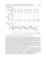
Figure 1 shows the inventory position of the retailer and the supplier between the time zero
(the time the supplier places the order Q
0
) and the time the same order (Q
0
) will be sent to
the retailer.

Information Sharing: a Quantitative Approach to a Class of Integrated Supply Chain

119
Supplier’s inventory
Position

m
Q

Q
m
=Q
Q
1
=Q
Q
0
=Q
(m+1)
Q=Q
m
Q
Q=Q
m-1
0
t
s
t
Q
t
s+Q
t
2Q
Q
Q=Q
m-2
t
s+2Q
Q

t
mQ
Q=Q
0
t
s+mQ
Time

Retailer’s inventory
Position

0
t
s
t
Q
t
s+Q
t
2Q
t
s+2Q
t
mQ
t
s+mQ
Time

R
R+Q

R+s

Fig. 1. Inventory position of the supplier and the retailer in [0,t
s+mQ
]
To prove this assertion, let us consider a time at which the supplier places an order to the
outside source. We designate this time as time zero. We also denote the batch which the
supplier orders at time zero by Q
0
. At this time, the retailer’s inventory position is exactly
Rs and the supplier’s inventory position will just reach(m+1)Q. Thus the batch Q
0
will fill
the (m+1)
th
demand for the retailer batch at the warehouse. We denote the arrival times of
customers who arrive after time zero by t
1
, t
2
, At time t
s
when the s
th
customer arrives, the
retailer will order one batch of size Q, and the supplier’s inventory position will drop to mQ.
We note that after time zero, at the arrival time of (s+mQ)
th
customer, i.e., at time t
s+mQ

, the
retailer will order a batch of size Q. This retailer’s order will be fulfilled by the (same) batch
Q
0
that was ordered by the supplier at time zero. This means that the batch Q
0
is released
from the warehouse when (s+mQ)
th
system demand has occurred after this order, i.e. after
time zero.
The first unit in the batch Q
0
will be used in the same way to fill the (R+1)
th
retailer demand
after the retailer order. Then the first unit in the batch Q
0
will have the same expected
retailer and warehouse costs as a unit in a base stock system with S
0
=s+mQ and S
1
=R+1.(the
first base stock system) Therefore the corresponding expected holding and shortage costs
will be equal to c(s+mQ , R+1) (A(12)).

Supply Chain Management – Pathways for Research and Practice

120

In the same way it can be seen that the j
th
unit in the batch Q
0
will be used to fill the (R+j)
th

retailer demand after the retailer order. Then the j
th
unit in the batch Q
0
will have the same
expected retailer and warehouse costs as a unit in a base stock system with S
0
=s+mQ and
S
1
=R+j.(j
th
base stock system) Therefore the expected holding and shortage costs for the j
th

unit in the batch Q
0
will be equal to c(s+mQ , R+j), j=1,…,Q (A(12)).
It should be noted that each customer, demands only one unit of a batch of size Q. If we
number the customers who use all Q units of this batch from 1 to Q, then the demand of any
customer will be filled randomly by one of these Q units. That is, each unit of a batch of size
Q will be consumed by the j
th

( j=1,2,…,Q) customer according to a discrete uniform
distribution on 1,2,…,Q. In other words, the probability that the i
th
(i=1,2,…,Q) unit of a
batch of size Q is used by the j
th
(j=1,2,…,Q) customer is equal to 1/Q. Therefore we can now
express the expected total cost for a unit demand as:

1
1
.( , )
Q
j
KcsmQRj
Q




(1)
Since the average demand per unit of time is equal to λ, the total cost of the system per unit
time can then be written as:

1
(,,) .
.( , )
Q
j
TC R m s K

cs mQR j
Q







(2)
which proves our assertion.
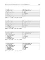
3. Model 2
In this section, we consider a three-echelon inventory system with two warehouses
(suppliers) and one retailer, as shown in Fig 2. This system usually called three-echelon
serial inventory system. We want to find the expected total holding and shortage costs for a
unit demand in three-echelon inventory system with two warehouses (suppliers) and one
retailer.


Fig. 2. Three-echelon Serial Inventory System
In this inventory system, transportation times from an outside source to the warehouse І,
between warehouses, and also from the warehouse II to the retailers are constant. We
assume that the retailer faces Poisson demand. Unfilled demand is backordered and the
shortage cost is a linear function of time until delivery, or equivalently, a time average of the
Echelon: (3) (2) (1)
Retailer
Warehouse I
I

Warehouse I

L
1

L
2

L
3


Information Sharing: a Quantitative Approach to a Class of Integrated Supply Chain

121
net inventory when it is negative. Each echelon follows a base stock, or (S-1, S), or one-for-
one replenishment policies. This means essentially that we assume that ordering costs are
low and can be disregarded.
The assumptions can be organized and presented as follows:
1. Transportation times between all locations are constant.
2. Arrival process of customer demand at the retailer is a Poisson process with a known
and constant rate.
3. Each customer demands only one unit of product.
4. There are linear holding costs at all locations and shortage cost in the retailer.
5. Replenishment policies are one-for-one.
6. Unfilled demand is backordered and the shortage cost is a linear function of time until
delivery.
7. Delayed retailer orders are satisfied on a first-come, first-served basis.
8. The outside source has ample capacity.
We fix the retailer, the warehouse II, and the warehouse I, to echelon one, two and three
respectively as shown in Fig. 2. In order to derive the cost function, the following notations
are used for serial inventory system:

S
i
Inventory position at echelon i in an inventory system with a one-for-one ordering policy
L
1
Transportation time from the Warehouse II to the retailer
L
2
Transportation time from the Warehouse I to the Warehouse II
L
3
Transportation time from the outside source to the Warehouse I (Lead time of the
Warehouse I)
T
i
Random delay incurred due to the shortage of stock at the echelon i (i=2,3)
λ Demand intensity at each echelon
h
i
Holding cost per unit per unit time at echelon i(i=1,2,3)
β Shortage cost per unit per unit time at the retailer
We characterizes our one-for-one replenishment policy by the (S
3
, S
2
, S
1
) of order-up-to
inventory positions which S
3

, S
2
, S
1
are the inventory position at warehouse I (echelon 3), the
inventory position at warehouse II (echelon 2), and the inventory position at retailer
(echelon 1), respectively. So we consider a one-for-one replenishment rule with (S
3
, S
2
, S
1
) as
the vector of order-up-to levels.
When a demand occurs at a retailer with a demand density, λ, a new unit is immediately
ordered from the warehouse II to warehouse I and also warehouse I immediately orders a
new unit at the same time, that is, each echelon faces the same demand intensity (λ). For the
one-for-one ordering policy as described above, any unit ordered by the retailer is used to
fill the S
1
th
demand following this order, hereafter, referred to as its demand. It means that,
an arbitrary customer consumes S
1
th
order placed by the retailer just before his arrival to the
retailer and we can also say that the customer consumes S
2
th
(S

3
th
) order placed by the
warehouse II (warehouse I) just before his arrival to the retailer. If the ordered unit arrives
prior to its (assigned) demand, it is kept in stock and incurs carrying cost; if it arrives after
its assigned demand, this customer demand is backlogged and shortage costs are incurred
until the order arrives. This is an immediate consequence of the ordering policy and of our
assumption that delayed demands and orders are filled on a first come, first served basis.
We confine ourselves to the case where all S
1
≥ 0.
To find the total cost, following the Axsäter’s (1990a) idea, let
(.)
i
S
i
g (i=1, 2, 3) denote the
density function of Erlang (λ, S
i
) distribution of the time elapsed between the placement of
an order and the occurrence of its assigned demand unit:

Supply Chain Management – Pathways for Research and Practice

122






ii
i
SS1
S
λ
t
i
i
λ t
g
(t) e
(S 1)!
(3)
The corresponding cumulative distribution function
()
i
S
i
Gtis:

()
()
!
i
i
k
S
t
i
kS

t
Gt e
k







(4)
An order placed by the retailer, arrives after L
1
+T
2
time units, and an order placed by
warehouse II, arrives after L
2
+T
3
time units, where T
i
(i=2,3) is the random delay
encountered at echelon i in case the echelon i is out of stock.
Let
1
2
1
()
S

t

denotes the expected retailer carrying and shortage costs incurred to fill a unit of
demand at retailer when inventory position at retailer is S
1
. We evaluate this quantity by
conditioning on T
2
= t
2
. Note that the conditional expected cost is independent of S
2
and S
3
,
and is given by:

12
11 1
12
212 1121
11 1
0
() ( ) () ( ) (), 0;
Lt
SS S
Lt
t L t sgsdsh sL tgsdsS






    

(5)
The conditional distribution of T
2
, on condition that T
3
=t
3
, obtained from:

2
2
23
1
()
23
233 23
2
0
()
01()
!
S
kk
S
Lt

k
Lt
PT T t e G L t
k






  

. (7)
Also the conditional density function f(T
2
) for 0 ≤ T
2
≤ L
2
+ t
3
is given by:

2
2
2 232
1
()
232
2233 232

2
2
()
()
(1)!
S
S
SLtt
Ltt
fT t T t g L t t e
S





 

(8)
The expression (6) shows the probability of time of receiving S
2
th
demand; that is after
receiving (S
2
-1)
th
demand, S
2
th

demand occurs at the time of L
2
+t
3
-t
2
. On the other view, we
can say the time distance between receiving S
2
th
demand and receiving the order from
warehouse I (L
2
+t
3
) is t
2
and we call it the delay time that occurred in warehouse II. As we
mentioned earlier the warehouses face a Poisson demand process with rate λ. Therefore we
use the expression (5) in third echelon as follows:

3
3
3
1
3
33
3
0
()

(0) 1 ()
!
S
kk
S
L
k
L
PT e G L
k





 

(9)
The density function f(t
3
) for 0 ≤ t
3
≤ L
3
,because we assume that inventory positrons at all
facilities in this system are equal or greater that zero, is given by:

3
3
3

33
1
()
33
333
3
3
()
() ( )
(1)!
S
S
S
Lt
Lt
ft g L t e
S







(10)
Let
1
32
1
(,)

S
SS denotes the expected retailer carrying and shortage costs incurred to fill a
unit of demand at retailer when
S
3
, S
2
, and S
1
are the inventory position at warehouse I,

Information Sharing: a Quantitative Approach to a Class of Integrated Supply Chain

123
warehouse II and the retailer, respectively. Considering both states that we have delay time
or have not in both warehouses, we obtain the cost that incurred to fill a unit of demand at
retailer, as follows:

2
3
12121
323
3
21 21
32 3 2 2 2 2 2
132121
0
33 232 22 23 3.
32121
00

(,)(1 ()) ( ) () (1 ()) (0)
( ) ( ) ( ) (1 ( ) (0))
L
S
SSSSS
LLt
S
SS SS
SS G L g L t tdt G L
gL t gL t t tdt GL t dt





  




  




(11)
The long-run average shortage and retailer carrying costs is clearly given by
1
32
1

(,)
S
SS

 .
The conditional expected warehouse
II holding cost,
2
3
2
()
s
t

, on condition that T
3
=t
3
, is
independent of
S
3
and given by:

22
23
32 23 2
22
() ( ) (), 0;
SS

Lt
th sLtgsdsS




 

(12)
Therefore we find the average warehouse holding cost per unit for warehouse II when the
inventory position at warehouse
I is S
3
as follows:

3
33
22 2
33333 3
232 32
0
() ( ) () (1 ()) (0).
L
SS
SS S
SgLttdt GL

  

(13)

Also the average warehouse
I holding costs per unit
3
()S

, which depends only on the
inventory position
S
3
is:

3
3
33 3
3
() ()( )
S
L
Sh
g
ss Lds




(14)
and
(0) 0

 .

We conclude that the long-run system-wide cost for the three-echelon serial inventory
system by adding the costs which occurred in each echelon and is given by:

12
321 32 3 3
12
C(S, S, S) ( (,) () ())
SS
SS S S

   (15)
3.1 Determination the economical policy of a three-echelon inventory system with
(R,Q) ordering policy and information sharing
In this section, we consider a three-echelon serial inventory system with two warehouses
(suppliers) and one retailer with information exchange. The retailer applies continuous
review (
R,Q) policy. The warehouses have online information on the inventory position and
demand activities of the retailer. The warehouse
I and II, start with m
1
and m
2
initial batches
of the same order size of the retailer, respectively. The warehouse
I places an order to an
outside source immediately after the retailer′s inventory position reaches an amount equal
to the retailer′s order point plus a fixed value
s
1
, and The warehouse II places an order to

Supply Chain Management – Pathways for Research and Practice

124
The warehouse I immediately after the retailer′s inventory position reaches an amount equal
to the retailer′s order point plus a fixed value
s
2
. Transportation times are constant and the
retailer faces independent Poisson demand. The lead times of the retailer and the warehouse
II, are determined not only by the constant transportation time but also by the random delay
incurred due to the availability of stock at the warehouses.
In order to find the total cost function for a unit demand in three echelon inventory system
with (
R,Q) ordering policy, first of all, we would present an (R,Q) ordering policy for a
system with two warehouses and one retailer as showed in Fig. 2.
In this section, we want to obtain this cost function by using the cost function presented by
the section 3, Hajiaghaei-keshteli and Sajadifar (2010), for the same system with one-for-one
ordering policy.
We use the following notations:
S
i
Echelon i inventory position in an inventory system with a one-for-one ordering policy
L
1
Transportation time from the Warehouse II to the retailer
L
2
Transportation time from the Warehouse I to the Warehouse II
L

3
Transportation time from the outside source to the Warehouse I (Lead time of the
Warehouse I)
λ Demand intensity at all echelons
h
i
Holding cost per unit per unit time at echelon i
β Shortage cost per unit per time at the retailer
c(S
3
,S
2
,S
1
) Expected total holding and shortage costs for a unit demand in an inventory
system with a one-for-one ordering policy
R The retailer′s reorder point
Q Order quantity at all locations
m
2
Number of batches (of size Q) initially allocated to the warehouse II
m
1
Number of batches (of size Q) initially allocated to the warehouse I
K Expected total holding and shortage costs for a unit demand
TC(R,m
1
,m
2
,s

1
,s
2
) Expected total holding and shortage costs of the system per time unit,
when the warehouse I and warehouse
II, start with m
1
and m
2
initial batches (of size Q), and
place an order in a batch of size
Q to upper source immediately after the retailer′s inventory
position reaches
R+s
1
and R+s
2
respectively.
As we shall see, with this approach we do not need to consider the parameters
L
i
, h
i
, and β
explicitly, but these parameters will, of course, affect the costs implicitly through the one-
for-one ordering policy costs.
When a demand occurs at the retailer, a new unit is immediately ordered from the
warehouse
II to the warehouse I and also the warehouse I immediately orders a new unit at
the same time.

If demands occur while the warehouses are empty, shipments are delayed. When units are
again available at the warehouses, delivered according to a first come, first served policy.
In such situation the individual unit is, in fact, already virtually assigned to a demand when
it occurs, that is, before it arrives at the warehouses. For the one-for-one ordering policy, an
arbitrary customer consumes (
S
1
+S
2
+S
3
)
th
, (S
1
+S
2
)
th
and S
1
th
, order placed by the warehouse
I, warehouse II, and the retailer, respectively, just before his arrival to the retailer.
If the ordered unit arrives prior to its (assigned) demand, it is kept in stock and incurs
carrying cost; if it arrives after its assigned demand, this customer demand is backlogged
and shortage costs are incurred until the order arrives. This is an immediate consequence of

Information Sharing: a Quantitative Approach to a Class of Integrated Supply Chain

125
the ordering policy and of our assumption that delayed demands and orders are filled on a
first come, first served basis.
To obtain
TC(R,m
1
,m
2
,s
1
,s
2
), we assume the warehouse I and II start with m
1
and m
2
initial
batches (of size
Q) respectively. The warehouse I places an order to an outside source
immediately after the retailer ′s inventory position reaches
R+s
1
, and warehouse II places an
order to warehouse I immediately after the retailer′s inventory position reaches
R+s
2
, while
s
1
is equal or greater than s

2
.
Let us consider a time that the warehouse
I places an order to the outside source. We set this
time equal to “A”. We also denote the batch which the warehouse
I orders at time “A” by
Q
A
. At this time, the retailer′s inventory position is just R+s
1
and the warehouse I′s inventory
position will just reach (
m
1
+1)Q.
After time “A”, when the retailer′s inventory position reaches
R+s
2
, warehouse II places an
order to the warehouse
I and her inventory position will just reach (m
2
+1)Q and warehouse I
′s inventory position will reach
m
1
Q. We set this time to “B”.
After time “B”, when s
2
th

customer demand arrives, that is, the retailer inventory position
reaches
R, the retailer will order one batch (of size Q), and the warehouse II′s inventory
position will reach
m
2
Q.
We note that after time “A”, at the arrival time of (
m
1
Q + s
1
- s
2
)
th
customer demand, the
warehouse
II will order a batch (of size Q). This warehouse II′s order will be fulfilled by the
(same) batch
Q
A
,

that was ordered by the warehouse I at time “A”, and after time “A´”, at
the arrival time of (
m
2
Q + s
2

)
th
customer demand, the retailer will order a batch (of size Q).
This warehouse
II′s order will be fulfilled by the (same) batch Q
B
that was ordered by the
warehouse
II at time “B”.
Besides after time “A”, At the arrival time of (
m
1
Q + m
2
Q + s
1
)
th
customer, the retailer will
order a batch of size
Q, this retailer′s order will be fulfilled by the same batch Q
A
that was
ordered by the warehouse
I at time “A”. Figure 3 shows the inventory position of the retailer
and the warehouses, as we detailed.
Furthermore, the (
R+1)
th
customer who arrives after this retailer′s order, will use the first

unit of this batch; this customer is (
m
1
Q+m
2
Q+s
1
+R+1)
th
customer who arrives after time
“A”. This customer will incur a cost equal to
c(m
1
Q+s
1
-s
2
, m
2
Q+s
2
, R+1), similar to c(S
3
,S
2
,S
1
),
see equation (A.8), in which
S

3
, S
2
, and S
1
are replaced by m
1
Q+s
1
-s
2
, m
2
Q+s
2
, and R+1,
respectively.
The
j
th
unit (j=1,2, …, Q) in the batch will have to wait for the (R+j)
th
customer who arrives
after this retailer′s order and it will incur a cost equal to
c(m
1
Q+s
1
-s
2

, m
2
Q+s
2
,R+j), similar to
(A.8), in which
S
3
, S
2
, and S
1
are replaced by m
1
Q+s
1
-s
2
, m
2
Q+s
2
, and R+j, respectively.
It should be noted that each customer demands only one unit of a batch of size
Q. if we
number the customer who use all
Q units of this batch from 1 to Q, then the demand of any
customer will be filled randomly by one of these
Q units. That is, each unit of a batch of size
Q will be consumed by the j

th
(j=1,2,…,Q) customer according to a discrete uniform
distribution between[
1,Q]. In other words, the probability that the i
th
unit of a batch of size Q
is used by
j
th
(j=1,2,…,Q) customer is equal to 1/Q.
Therefore we can now express the expected total cost for a unit demand as:

1
K ( , , )
11222
1
Q
cmQs smQsRj
Q
j

  


(16)

Supply Chain Management – Pathways for Research and Practice

126

Fig. 3. Inventory position of the supplier and the warehouses

Information Sharing: a Quantitative Approach to a Class of Integrated Supply Chain

127
Since the average demand per unit of time is equal to λ, the total cost of the system per unit
time can then be written as:

1212 1 122 2
1
TC(R,m ,m ,s ,s ) . ( , , )
Q
j
KcmQssmQsR
j
Q






(17)
4. Model 3
In this section, we consider a single item, two-level inventory system which consisting of
two suppliers and one retailer, as shown in Fig 4. Transportation times are constant. The
retailer faces Poisson demands and applies continuous (
R, Q) policy. Each supplier starts
with m initial batches of size
Q/2 and places an order in a batch of size Q/2 to an outside

source immediately after the retailer’s inventory position reaches
R+s. (Sajadifar et. al, 2008)


Fig. 4. A convergent two-level inventory system
4.1 Problem formulation
The following notations are used for this system:
S
0
Suppliers inventory position in an inventory system with a one- for-one ordering policy
S
1
Retailer inventory position in an inventory system with a one-for-one ordering policy
L
i
Transportation times from the supplier i to the retailer
L
0
i
Transportation times from the outside source to the supplier i (Lead time of the supplier)
λ Demand intensity at the retailer
h Holding cost per unit per unit time at the retailer
h
0
i
Holding cost per unit per unit time at the supplier i
β Shortage cost per unit per unit time at the retailer
t
k
Arrival time of the k

th
customer after time zero
ω
i
Random delay incurred due to the shortage of stock at the supplier i
X
i
Lead time of the retailer when she receives a bath from the path i
P
ij
The probability that path i is shorter than path j.
g
n
(t) Density function of the Erlang (λ, n)
G
n
(t) Cumulative distribution function of g
n
(t)
c
i
(S
0
, S
1
) Expected total holding and shortage costs for a unit demand in an inventory
system with a one-for-one ordering policy in path
i.
R The retailer’s reorder point
Q

Order quantity at the retailer
m Number of batches (of sizeQ/2) initially allocated to the suppliers
K Expected total holding and shortage costs for a unit demand

Supply Chain Management – Pathways for Research and Practice

128
TC(R,m,s)Expected total holding and shortage costs of the system per time unit, when the
suppliers starts with
m initial batches (of size Q/2), and places an order in a batch of size Q/2
to outside sources immediately after the retailer’s inventory position reaches
R+s.
It can be seen that X
i
= L
i
+ ω
i
. To find K, we express it as a weighted mean of costs for the
one-for-one ordering policies. As we shall see, with this approach we do not need to
consider the parameters
L
i
,L
0
i
, h, h
0
i
, β and λ explicitly, but these parameters will, of course,

affect the costs implicitly through the one-for-one ordering policy costs. To derive the one-
for-one carrying and shortage costs, we suggest the recursive method in (Axsäter,1990a).
Also, we consider the following assumptions:
1. Orders do not cross,
i.e. all orders/portions have arrived when the reorder point is
reached and new orders are placed.
2. Each customer demands only one unit of product.
3. Each path that starts from outside source of the supplier i and end to the retailer is
named by the path i. In other words the retailer receives each batch that shipped by the
supplier
i from the path i (i=1, 2).
4. Delayed retailer orders are satisfied on a first-come, first-served basis.
4.2 Deriving model
In this section, we use the method that (Haji and Sajadifar ,2008) introduced for evaluating
the exact expected total costs of the inventory system, i.e., the exact expected total holding
and shortage costs per time unit,
TC(R,m,s). To obtain TC(R,m,s), using the (Axsäter,1990a)
exact solutions for Poisson models with one-for-one ordering policies they show that the
expected holding and shortage costs for the order of the
j
th
customer is exactly equal to the
total costs for a unit demand in a base stock system with suppliers and retailer’s inventory
positions
S
0
=s+mQ and S
1
=R+j and so is equal to c(s+mQ, R+j).(A.12)
Figure 5 shows the inventory position of the retailer and the each supplier between the time

zero (the time the each supplier places the order
Q
0
/2) and the time the same order (Q
0
/2)
will be sent to the retailer.
Let us consider a time that inventory position of the retailer reaches to ‘
R+s’. We designate
this time as time zero. At this time, the suppliers immediately place an order equal to
Q/2 to
the outside sources. We denote this batch by
Q
0
/2. At this time, the retailer’s inventory
position is exactly
R+s and the suppliers' inventory positions will just reach (m+1)Q/2. Since
we assume that the orders do not cross, the (
m+1)
th
order at the retailer will release the
orders
Q
0
/2 at the suppliers. It can be easily seen that the (s+mQ)
th
customer at the retailer
will be caused to an order placement at the retailer and the one which has been already
assigned to this order at the suppliers are the batches
Q

0
/2. This means that the batch Q
0
/2 at
each suppliers, is released from the warehouse when (
s+mQ)
th
system demand has occurred
after time zero i.e. at
t
s+mQ
.
The batch
Q
0
/2 will be received from the path i earlier than the batch Q
0
/2 from the path j
with the probability
P
ij
. Therefore, the first unit in the batch Q
0
/2 (which will be received
from path
i) will be used in the same way to fill the (R+1)
th
retailer demand after the retailer
order. Then the first unit in the batch
Q

0
/2 will have the same expected retailer and
warehouse costs as a unit in a base stock system with
S
0
=s+mQ and S
1
=R+1 (Haji and
Sajadifar 2008). Hence the corresponding expected holding and shortage costs will be equal
to
c
i
(s+mQ , R+1) (A(12)).