Tribology Lubricants and Lubrication 2012 Part 7 pdf
Bạn đang xem bản rút gọn của tài liệu. Xem và tải ngay bản đầy đủ của tài liệu tại đây (4.06 MB, 25 trang )
Tribology - Lubricants and Lubrication
142
With the use of the pipeline fixing (type a), tests of the pipe dug out of soil (in the air) are
modeled. The stress-strain state of a pipe lying in hard soil without friction in the axial
direction is modeled by means of pipe fixing (type b) while that of a pipe lying in hard soil
and rigidly connected with it – by means of pipe fixing (type c). Subject to boundary
conditions (8) (type d), a pipe lying in soil having particular mechanical characteristics is
modeled.
Thus, the problem has been stated to make a comparative analysis of the stress-strain states
of the pipe with corrosion damage for different combinations of boundary conditions (1)–
(3), (6)–(8):
() ()
() () () ()
()()()( )( )( )
,;,; ,;
,; ,; , .
pp
TT
ij ij ij ij ij ij
pp p
T
p
T
p
T
p
T
ij ij ij ij ij ij
ττ
ττ τ τ
σεσεσε
σεσεσ ε
+ + + + ++ ++
(9)
where the superscripts p, τ, and T correspond to the stress states caused by internal
pressure, friction force over the inner surface of the pipe, and temperature.
In the case of the elastic relationship between stresses and strains, the stress states in (9) are
connected by the following relations
() ()
()
() ()
()
()()
() ( )
,
,
.
pp
ij ij ij
pT p
T
ij ij ij
pT p
T
i
j
i
j
i
j
i
j
τ
τ
τ
τ
σσσ
σσσ
σσσσ
+
+
++
=+
=+
=++
(10)
Further, some of the solutions to more than 70 problems of studying the stress-strain state of
the pipe cross section in the damage area (dot-and-dash line in Figure 1) [Kostyuchenko et
al., 2007a; 2007b; Sherbakov et al., 2007b; 2008a; 2008b; Sherbakov, 2007b; Sosnovskiy et al.,
2008] are analyzed. These two-dimensional problems mainly describe the stress-strain states
of straight pipes with different-profile damage along the axis. Also, with the use of the
finite-element method implemented in the software ANSYS, the essentially three-
dimensional stress-strain state of the pipe in the three-dimensional damage area (Figure 1)
was investigated.
3. Wall friction in the turbulent mineral oil flow in the pipe with corrosion
damage
Within the framework of the present work, hydrodynamic calculation was made of the
motion characteristics of a viscous, incompressible, steady, isothermal fluid in a cylindrical
channel that models a pipe and in a cylindrical channel with geometric characteristics with
regard to the peculiarities of a pipe with corrosion damage (see, Sect. 2). Calculations were
performed for the initial incoming flow velocities υ
0
: 1 m/sec and 10 m/sec.
The kinematic viscosity of fluid was taken equal to v
K
= 1.4 10
-4
m
2
/sec, the viscous fluid
density – 865 kg/m
3
. The calculated Reynolds numbers will be, respectively,
0
1m/sec
42
1m /sec*0.612m
Re 4371.43,
1.4*10 m /sec
K
D
υ
ν
−
== = (11)
Three-Dimensional Stress-Strain State of a Pipe with Corrosion Damage Under Complex Loading
143
0
10 m/sec
42
10m /sec*0.612m
Re 43714.3.
1.4*10 m /sec
K
D
υ
ν
−
== =
(12)
The critical Reynolds number (a transition from a laminar to a turbulent flow) for a viscous
fluid moving in a round pipe is Re
cr
≈ 2300. Thus, the turbulent flow motion should be
considered in our problem. The software Fluent calculations used the turbulence k – ε model
for modeling turbulent flow viscosity [Launder et al., 1972; Rodi, 1976].
As boundary conditions the following parameters were used: at the incoming flow surface
the initial turbulence level equal to 7% was assigned; at the pipe walls the fixing conditions
and the logarithmic velocity profile were predetermined; in the pipe the fluid pressure equal
to 4 МPа was set.
Calculations of the steady regime of the fluid flow (quasi-parabolic turbulent velocity profile
of the incoming flow) and of the unsteady regime (rectangular velocity profile of the
incoming flow) were made.
In the problems with a rectangular velocity profile of the incoming flow
1
0
,
xr
x
υ
υ
=
= (13)
The unsteady regime of the fluid flow was considered.
In the problems with a quasi-parabolic turbulent velocity profile, at the entrance surface of
the pipe the empirically found profile of the initial velocity was assigned, which is
determined by the formula:
-
for the two-dimensional case
1
7
0
max max 0 1
0
0
2
1 , 1.1428 ,0 2 ,
2
x
x
rr
rr
r
υυ υ υ
=
⎛⎞
−
=− = ≤≤
⎜⎟
⎝⎠
(14)
-
for the three-dimensional case
1
7
22
max max 0 1
0
0
1 , 1.2244 , ,0 .
x
x
r
ry z rr
r
υυ υ υ
=
⎛⎞
=
−==+≤≤
⎜⎟
⎝⎠
(15)
The calculation results have shown that the motion becomes steady (as the flow moves in
the pipe, the quasi-parabolic turbulent profile of the longitudinal velocity V
x
develops) at
some distance from the entrance (left) surface of the pipe (Figure 3). So, from Figure 4 it is
seen that for the quasi-parabolic velocity profile of the incoming flow the zone of the steady
motion begins earlier than for the rectangular profile.
Further, we will consider the results obtained for the velocity profiles of the incoming flow
calculated in accordance to (14) and (15).
Consider the flow turbulence intensity being the ratio of the root-mean-square fluctuation
velocity u′ to the average flow velocity u
avg
(Figure 5).
'
,
av
g
u
I
u
=
(16)
At the surface of the incoming flow, the turbulence intensity is calculated by the formula
Tribology - Lubricants and Lubrication
144
()
1
0
8
0.16 Re , Re ,
HH
H
DD
D
I
υ
ν
−
== (17)
where D
H
is the hydraulic diameter (for the round cross section: D
H
= 2r
1
= 0.612 m), υ
0
is the
incoming flow velocity, and v is the kinematic viscosity of oil (v = 1.4⋅10
–4
m
2
/sec).
Fig. 3. Longitudinal velocity V
x
(two-dimensional flow) for the quasi-parabolic turbulent
velocity profile of the incoming flow at υ
0
= 1 m/sec
Fig. 4. Profiles of the longitudinal velocity V
x
. over the pipe cross sections (three-dimensional
flow) for the quasi-parabolic turbulent velocity profile of the incoming flow at υ
0
= 1 m/sec
Three-Dimensional Stress-Strain State of a Pipe with Corrosion Damage Under Complex Loading
145
Fig. 5. Turbulence intensity (two-dimensional pipe flow, quasi-parabolic turbulent velocity
profile, υ0 = 1 m/sec)
Fig. 6. Transverse velocity V
y
for the two-dimensional flow in the pipe with corrosion
damage at υ0 = 10 m/sec
The zone of the unsteady turbulent motion is characterized by the higher turbulence
intensity (vortex formation) in comparison with the remaining region of the pipe (Figure 5).
The highest intensity is observed in the steady motion zone, which is especially noticeable in
the calculations with the initial velocity of 1 m/sec in the pipe wall region, whereas the
lowest one – at the flow symmetry axis.
At high initial flow velocity values the vortex formation rate is higher.
Tribology - Lubricants and Lubrication
146
It should be emphasized that at a higher value of the initial flow velocity, the instability
region is longer: at υ
0
= 1 m/sec its length is about 2 m, while at υ
0
= 10 m /sec its length is
about 5 m.
The behavior of the motion (steady or unsteady) exerts an influence on the value of wall
stresses. In the unsteady motion zone, they are essentially higher as against the appropriate
stresses in the identical steady motion zone.
These figures illustrate that at that place of the pipe, where the fluid motion becomes steady,
the value of tangential stress at υ
0
= 1 m/sec is approximately equal to 8 Pa, whereas at υ
0
=
10 m/sec it is about 240 Pa.
The results as presented above are peculiar for a pipe with corrosion damage and without it.
At the same time, the presence of corrosion damage affects the kinematics of the moving
flow in calculations with both the rectangular profile of the initial flow velocity and the
quasi-parabolic turbulent one. In this domain of geometry, there appear transverse
displacements that form a recirculation zone (Figure 7).
Fig. 7. Transverse velocity V
z
for the three-dimensional flow in the pipe with corrosion
damage at υ
0
= 10 m/sec
The corrosion spot exerts a profound effect on changes in wall tangential stresses in the area
of the pipe corrosion damage.
Figures 8 and 9 demonstrate that in the corrosion damage area, the values of wall tangential
stresses undergo jumping.
For the laminar fluid motion, the value of tangential stresses at the pipe wall is calculated by
the following formula [Sedov, 2004]:
0
0
0
4
,
y
x
d
yx drr
υ
υ
μυ
υ
τμ μ
∂
⎛⎞
∂
=+==
⎜⎟
⎜⎟
∂∂
⎝⎠
(18)
where μ = υ⋅ρ = 1.4⋅10
–4
⋅865 = 0.1211 kg/(m*sec) is the molecular viscosity, r
0
= 0.306 m is the
pipe radius.
Three-Dimensional Stress-Strain State of a Pipe with Corrosion Damage Under Complex Loading
147
Fig. 8. Wall tangential stresses at the pipe wall: stresses at y = f(x), stresses at y = 2r
1
for the
two-dimensional flow in the pipe with corrosion damage at υ
0
= 1 m/sec
Fig. 9. Wall tangential stresses at the pipe wall: stresses at y = f(x), stresses at y = 2r
1
for the
two-dimensional flow in the pipe with corrosion damage at υ
0
= 10 m/sec
Then τ
0
for the velocities υ
0
= 10 m/sec and υ
0
= 1 m/sec will be
10 1
00
4 0.1211 10 4 0.1211 1
15.83 Pa, 1.58 Pa.
0.306 0.306
ττ
⋅⋅ ⋅⋅
====
(19)
The expression for the tangential stresses with regard to the turbulence is of the form
[Sedov, 2004]:
0
'''().
yy
xx
xy xy x y t
y
xyx
υυ
υυ
τττ μ ρυυ μμ
∂∂
⎛⎞ ⎛⎞
∂∂
=+ = + − = + +
⎜⎟ ⎜⎟
⎜⎟ ⎜⎟
∂∂ ∂∂
⎝⎠ ⎝⎠
(20)
The last formula and the analysis of the calculations enable evaluating the turbulence
influence on the value of tangential stresses at the pipe wall. As indicated above, at different
profiles and initial velocity values the tangential stresses were obtained: at υ
0
= 1 m/sec:
Tribology - Lubricants and Lubrication
148
τ
xy
= τ
w
≈ 8 Pa, at υ
0
= 10 m/sec: τ
xy
= τ
w
≈ 240 Pa. The value of the turbulent stress (Reynolds
stress):
at υ
0
= 1 m/sec :
0
' ' ' 8 1.58 6.42Pa,
y
x
xy x y t xy
yx
υ
υ
τρυυμ ττ
∂
⎛⎞
∂
=− = + = − = − =
⎜⎟
⎜⎟
∂∂
⎝⎠
(21)
at υ
0
= 10 m/sec :
0
'''
240 15.83 224.17 Pa,
y
x
xy x y t xy
yx
υ
υ
τρυυμ ττ
∂
⎛⎞
∂
=
−=+=−=
⎜⎟
⎜⎟
∂∂
⎝⎠
=− =
(22)
The results obtained are evident of the fact that the turbulence much contributes to the
formation of wall tangential stresses. At the higher turbulence intensity (it is especially high
in the pipe wall region), Reynolds stresses increase, too. I.e., the turbulence stresses are:
at υ
0
= 1 m/sec :
0
81.58
100% 100% 80.25%;
8
xy
xy
τ
τ
τ
−
−
==
(23)
at υ
0
= 10 m/sec :
0
240 15.83
100% 100% 93.4%.
240
xy
xy
τ
τ
τ
−
−
==
(24)
The analysis as made above shows that the calculation of the motion of a viscous fluid in the
pipe as laminar can result in a highly distorted distribution pattern of the tangential stresses
at the inner surface of the pipe. It can be concluded that the analysis of viscous fluid friction,
when the flow interacts with the pipe wall, must be performed on the basis of the
calculation of flow motion as essentially turbulent one.
4. Analytical solutions for the stress-strain state of the pipeline model under
the action of internal pressure and temperature difference
In the simplified analytical statement, the problem of calculating the stress-strain state of a
long cylindrical pipe reduces to the problem of the strain of a thin ring loaded with a
pressure p
1
uniformly distributed over its inner wall and also with a pressure p
2
uniformly
distributed over the outer surface of the ring (Figure 10). Operating conditions of the ring do
not vary depending on whether it is considered either as isolated or as a part of the long
cylinder.
Work [Ponomarev et al., 1958] and many other publications contain the classical solution to
this problem based on solving the following differential equation for radial displacements:
2
22
11
0.
rr
r
du du
u
rdr
dr r
+
−=
(25)
The general solution of this equation is of the form:
12
1
.
r
uCrC
r
=+
(26)
Three-Dimensional Stress-Strain State of a Pipe with Corrosion Damage Under Complex Loading
149
With the use of the relationship between stresses and strains, and also of Hook’s law, it is
possible to determine integration constants С
1
and С
2
under the boundary conditions of the
form:
1
2
1
2
,
.
r
rr
r
rr
p
p
σ
σ
=
=
=−
=−
(27)
where р
1
is the internal pressure; р
2
is the external pressure.
Fig. 10. Loading diagram of the circular cavity of the pipe
In such a case, the general formulas for stresses at any pipe point have the following form:
22 22
11 22 1 2 12
22 22 2
21 21
22 22
11 22 1 2 12
22 22 2
21 21
()
1
,
()
1
.
r
pr pr p p rr
rr rr r
pr pr p p rr
rr rr r
ϕ
σ
σ
−−
=−
−−
−−
=+
−−
(28)
Assuming that the cylinder is loaded only with the internal pressure (р
1
= p, р
2
= 0), the
following expressions are obtained for the stresses based on the internal pressure:
()
()
22
12 12
22 22
212 212
11
1, 1,
11
p
p
rr r
rr rr
kk
pp
kk kk
ϕ
σ
σ
⎛⎞ ⎛⎞
=−=+
⎜⎟ ⎜⎟
⎜⎟ ⎜⎟
−−
⎝⎠ ⎝⎠
(29)
where k
r2
= r /r
2
, k
r12
= r
1
/ r
2
To analyze the rigid fixing of the outer surface of the pipeline, as one of the equations of the
boundary conditions we choose expression (26) for displacements, the value of which tends
to zero at the outer surface of the model. As the secondary boundary condition we use an
expression for stresses at the inner surface of the cylinder from (27):
12
1
, 0.
rr
rr rr
pu
σ
==
=
−= (30)
Then, the expressions for the stresses will assume the form:
Tribology - Lubricants and Lubrication
150
(
)
()
22
12 2 1 1
22
212 1 1
22
12 2 1 1
22
212 1 1
(1 ) ( 1)
,
(1 ) ( 1)
(1 ) ( 1)
.
(1 ) ( 1)
p
rrr
rr
p
rr
rr
kk
p
kk
kk
p
kk
ϕ
σνν
νν
σ
νν
νν
+−−
=−
+−−
++−
=−
+−−
(31)
Consider a long thick-wall pipe, whose wall temperature t varies across the wall, but is
constant along the pipe, i. e., t = t(r) [Ponomarev et al., 1958].
If the heat flux is steady and if the temperature of the outer surface of the pipe is equal to
zero and that of the inner surface is designated as Т, then from the theory of heat transfer it
follows that the dependence of the temperature t on the radius r is given by the formula
2
12
ln ,
ln
r
r
T
tk
k
= (32)
Any other boundary conditions can be obtained by making uniform heating or cooling,
which does not cause any stresses. Thus, the quantity Т in essence represents the
temperature difference ΔT of the inner and outer surfaces of the pipe.
As the temperature is constant along the pipe, it can be considered that cross sections at a
sufficient distance from the pipe ends remain plane, and the strain ε
z
is a constant quantity.
The temperature influence can be taken into account if the strains due to stresses are added
with the uniform temperature expansion Δε = αΔT where α is the linear expansion
coefficient of material.
The stress-strain state in the presence of the temperature difference between the pipe walls
can be determined by solving the differential equation [Ponomarev et al., 1958]:
2
1
22
1
11
.
1
du du u dt
rdr dr
dr r
ν
α
ν
+
+−=
−
(33)
Subject to the boundary conditions
12
0, 0.
rr
rr rr
σσ
==
=
= (34)
Having solved boundary-value problem (33), (34), the expressions for stresses are of the
form:
()
()
()
()
()
()
2
12
1
212
22
12 12 2
2
12
1
212
22
12 12 2
2
12
1
212
2
12 12
11
ln 1 ln ,
21
ln 1
11
1ln 1 ln ,
21
ln 1
2
1
1 2ln ln ,
21
ln 1
T
r
rrr
rrr
T
r
rr
rrr
T
r
zrr
rr
k
ET
kk
kkk
k
ET
kk
kkk
k
ET
kk
kk
ϕ
α
σ
ν
α
σ
ν
α
σ
ν
⎡⎤
⎛⎞
Δ
=−−−
⎢⎥
⎜⎟
⎜⎟
−
−
⎢⎥
⎝⎠
⎣⎦
⎡
⎤
⎛⎞
Δ
=−−−+
⎢
⎥
⎜⎟
⎜⎟
−
−
⎢
⎥
⎝⎠
⎣
⎦
⎡⎤
Δ
=−−−
⎢⎥
−
−
⎢⎥
⎣⎦
(35)
Figures 11–14 show the distribution of dimensionless stresses (29), (31), (35) along r and
their sums
Three-Dimensional Stress-Strain State of a Pipe with Corrosion Damage Under Complex Loading
151
() ()
()
,,,,
pT p
T
iii
ir z
σσσ ϕ
+
=+ = (36)
for k
r12
= 0.8, v = 0.3, E
1
αT / p = 10 (for example, at E
1
= 2⋅10
11
Pa, α = 10
-
5°С
-1
, ΔT = 20 °C).
These figures well illustrate the essential influence of the temperature and the procedure of
fixing the pipe on its stress-strain state.
Fig. 11. Radial stresses for problems (25), (27) and (33), (34) at r1 ≤ r ≤ r2
Compare the distribution of the stresses calculated analytically with the use of (31) for a
non-damaged pipe with the finite-element calculation results by plotting the graphs of the
pipe thickness stress distribution (Figures 1.15–1.16). To make calculation, take the following
initial data: inner and outer radii r
1
= 0.306 m and r
2
= 0.315 m, p
1
= 4М Pa, p
2
= 0, Е = 2⋅10
11
Pa,
ν = 0.3.
Fig. 12. Circumferential stresses for problems (25), (27) and (33), (34) at r1 ≤ r ≤ r2
Tribology - Lubricants and Lubrication
152
Fig. 13. Longitudinal stresses for problems (25), (30) and (33), (34) at r1 ≤ r ≤ r2
Fig. 14. Circumferential stresses for problems (25), (30) and (33), (34) at r1 ≤ r ≤ r2
As seen from Figures 15–16, the σ
r
and σ
ϕ
distributions obtained from the analytical
calculation practically fully coincide with those obtained from the finite-element calculation,
which points to a very small error of the latter.
5. Stress-strain state of the three-dimenisonal model of a pipe with corrosion
damage under complex loading
Consider the problem of determining the stress-strain state of a two-dimenaional model of a
pipe in the area of three-dimensional elliptical damage.
In calculations we used a model of a pipe with the following geometric characteristics
(Figure 2): inner (without damage) and outer radii r
1
= 0.306 m and r
2
= 0.315 m,
Three-Dimensional Stress-Strain State of a Pipe with Corrosion Damage Under Complex Loading
153
Fig. 15. Radial stress distribution for the analytical calculation (
()
p
r
σ
), for the two-
dimensional computer model (
(
)
2D
r
σ
), for the three-dimensional computer model (
()
3D
r
σ
)
Fig. 16. Circumferential stress distribution for the analytical calculation (
()
p
ϕ
σ
), for the two-
dimensional computer model (
(
)
2D
ϕ
σ
), for the three-dimensional computer model (
()
3D
ϕ
σ
)
respectively, the length of the calculated pipe section L=3 m, sizes of elliptical corrosion
damage length × width × depth – 0.8 m × 0.4 m × 0.0034 m.
The pipe mateial had the following characteristics: elasticity modulus E
1
= 2⋅10
11
Pa,
Poisson’s coefficient v
1
= 0.3, temperature expansion coefficient α = 10
-5
°С
-1
, thermal
conductivity k = 43 W/(m°С), and the soil parameters were: E
2
= 1.5⋅10
9
Pa, Poisson’s
coefficient v
2
= 0.5. The coefficient of friction between the pipe and soil was μ = 0.5.
The internal pressure in the pipe (1) is:
1
4 MPa.
r
rr
p
σ
=
== (37)
Tribology - Lubricants and Lubrication
154
The temperature diffference between the pipe walls is (3)
12
20 .
о
rr
TT T С−=Δ= (38)
The value of internal tangential stresses (wall friction) (2) is determined from the
hydrodynamic calculation of the turbulent motion of a viscous fluid in the pipe.
Calculations in the absence of fixing of the outer surface of the pipe and in the presence of
the friction force over the inner surface (2) were made for 1/2 of the main model (Figure 2),
since in this case (in the presence of friction) the calculation model has only one symmetry
plane. In the absence of outer surface fixing, calculations were made for 1/4 of the model of
the pipeline section since the boundary conditions of form (2) are also absent and, hence, the
model has two symmetry planes.
The investigation of the stress state of the pipe in soil is peformed for 1/4 of the main model
of the pipe placed inside a hollow elastic cylinder modeling soil (Figure 17).
In calculations without temperature load, a finite-element grid is composed of 20-node
elements SOLID95 (Figure 17) meant for three-dimensional solid calculations. In the
presence of temperature difference, a grid is composed of a layer of 10-node finite elements
SOLID98 intended for three-dimensional solid and temperature calculations. The size of a
finite element (fin length) a
FE
=10
-2
m.
Fig. 17. General view and the finite-element partition of ¼ of the pipe model in soil
Thus, the pipe wall is composed of one layer of elements since its thickness is less than
centermeter. During a compartively small computer time such partition allows obtaining the
results that are in good agreement with the analytical ones (see, below).
Calculations for boundary conditions (8) with a description of the contact between the pipe
and soil use elements CONTA175 and TARGE170.
As seen from Figure 17, the finite elements are mainly shaped as a prism, the base of which
is an equivalateral triangle. The value of the tangential stresses
1
rz
rr
τ
=
applied to each node
of the inner surface will then be calculated as follows:
1
()
0
,
node
rz
rr
S
τ
τ
=
= (39)
where S is the area of the romb with the side a
FE
and with the acute angle β
FE
= π/3. Thus,
the value of the tangential stress applied at one node will be
Three-Dimensional Stress-Strain State of a Pipe with Corrosion Damage Under Complex Loading
155
1
()
242
0
sin 260 10 3 /2 2.25 10 Pa.
node
rz FE FE
rr
a
ττβ
−−
=
==⋅=⋅ (40)
The analysis of the calculation results will be mainly made for the normal (principal)
stresses σ
x
, σ
y
, σ
z
in the Cartesian system of coordinates. It should be noted that for axis-
symmetrical models, among which is a pipe, the cylindrical system of coordinates is natural,
in which the normal stresses in the radial σ
r
, circumferential σ
t
, and axial σ
z
directions are
principal. Since the software ANSYS does not envisage stresses in the polar system of
coordinates, the analysis of the stress state will be made on the basis of σ
x
, σ
y
, σ
z
in those
domains where they coincide with σ
r
, σ
t
, σ
z
corresponding to the last principal stresses σ
1
,
σ
2
, σ
3
and also to the tangential stresses σ
yz
.
Make a comparative analysis of the results of numerical calculation for boundary conditions
(1), (6) and (1), (7) with those of analytical calculation as described in Sect. 1.4. Consider pipe
stresses in the circumferential σ
t
and radial σ
r
directions.
Figures 18 and Figure 19 show that in the case of fixing
2
2
0
xy
rr
rr
uu
=
=
=
= , corrosion
damage exerts an essential influence on the σ
t
distribution over the inner surface of the pipe.
At the damage edge, the absolute value of circumferential σ
t
is, on average, by 15% higher
than the one at the inner surface of the pipe with damage and, on average, by 30 % higher
than the one inside damage. In the case of fixing
22
2
0
xyz
rr rr
rr
uuu
==
=
=
==, the σ
t
distributions are localized just in the damage area. The additional key condition
2
0
z
rr
u
=
=
(coupling along the z-axis) is expressed in increasing |σ
t
| at the inner surface without
damage in the calculation for (1), (7) approximately by 60% in comparison with the
calculation for (1), (6). However in the calculation for (1), (7), the |σ
t
| differences between
the damage edge, the inner surface without damage, and the inner surface with damage are,
on average, only 6 and 3% , respectively. Maximum and minimum values of σ
t
in the
calculation for (1), (6) are:
min 6
1.27 10
t
σ
=− ⋅ Pa and
max 5
7.96 10
t
σ
=− ⋅ Pa; in the calculation
for (1), (7) are:
min 6
1.72 10
t
σ
=− ⋅ Pa and
max 6
1.61 10
t
σ
=
−⋅ Pa.
The analysis of the stress distribution reveals a good coincidence of the results of the
analytical and finite-element calculations for σ
t
. At r
1
≤ y ≤ r
2
, x=z=0 in the vicinity of the
pipe without damage, the error is at r = r
1
1.093 1.082
100% 1.03%,
1.093
e
−
=⋅=
(41)
at r = r
2
1.175 1.165
100% 0.94%.
1.175
e
−
=⋅=
(42)
Thus, at the upper inner surface of the pipe the damage influence on the σ
t
variation is
inconsiderable. A comparatively small error as obtained above is attributed to the fact that
the three-dimensional calculation subject to (1), (6) was made at the same key conditions as
the analytical calculation of the two-dimensional model. At the same time, owing to the
additonal condition
2
0
z
rr
u
=
=
the difference between the results of the analytical
calculation and the calculation for (1), (7) is much greater – about 45 %.
Tribology - Lubricants and Lubrication
156
Fig. 18. Distribution of the stress σ
2
(σ
t
) at
1
r
rr
p
σ
=
=
,
2
2
0
xy
rr
rr
uu
=
=
=
=
Fig. 19. Distribution of the stress σ
1
(σ
t
) at
1
r
rr
p
σ
=
=
,
22
2
0
xyz
rr rr
rr
uuu
==
=
=
==
A more detailed analysis of the stress-strain state can be made for distributions along the
below paths.
For 1/2 of the pipe model:
Path 1. Along the straight line r
1
≤ y ≤ r
2
at x=z=0:
from P
11
(0, r
1
, 0) to P
12
(0, r
2
, 0).
Path 2. Corrosion damage center (– r
1
– h ≤ y ≤ – r
2
at x=z=0):
from P
21
(0, – r
1
– h, 0) to P
22
(0, – r
2
, 0).
Three-Dimensional Stress-Strain State of a Pipe with Corrosion Damage Under Complex Loading
157
Path 3. Cavity boundary over the cross section z=0:
from P
31
(0.186, – 0.243, 0) to P
32
(0.192, – 0.25, 0).
Path 4. Cavity boundary over the cross section x=0:
from P
41
(0, –r
1
, d/2) to P
42
(0, –r
2
, d/2).
Path 5. Along the straight line of the upper inner surface of the pipe
– 0.8L/2 ≤ z ≤ 0.8L/2 at x = 0, y = r
1
: from P
51
(0, r
1
, – 0.8L/2) to P
52
(0, r
1
, 0.8L/2).
Path 6. Along the curve of the lower inner surface of the pipe – 0.8L/2 ≤ z ≤ 0.8L/2 at x=0,
(
)
1
1
,0 /2
,/2 0.8/2
rfz zd
y
rd z L
⎧
−= ≤ ≤
⎪
=
⎨
−≤≤
⎪
⎩
through the points:
P
64
(0, – r
1
, – 0.8L/2), P
63
(0, – r
1
, – d/2), P
62
(0, – r
1
, – 0.0025, –0.2), P
61
(0, – r
1
, – h, 0), P
62
(0, – r
1
, –
0.0025, 0.2), P
63
(0, – r
1
, d/2), P
64
(0, – r
1
, 0.8L/2).
For 1/4 of the pipe model, paths 1–4 are the same as those for 1/2, whereas paths 5 and 6
are of the form:
Path 5. Along the strainght upper inner surface of the pipe 0 ≤ z ≤ 0.8L/2 at x=0, y=r
1
: from
P
51
(0, r
1
, 0) to P
52
(0, r
1
, 0.8L/2).
Path 6. Along the curve of the lower inner surface of the pipe 0 ≤ z ≤ 0.8L/2 at x=0,
()
1
1
,0 /2
,/2 0.8/2
rfz zd
y
rd z L
⎧− = ≤ ≤
⎪
=
⎨
−≤≤
⎪
⎩
through the points:
P
61
(0, – r
1
, – h, 0), P
62
(0, – r
1
, – 0.0025, 0.2), P
63
(0, – r
1
, d/2), P
64
(0, – r
1
, 0.8L/2).
In the above descriptions of the paths, d=0.8 m is the length of corrosion damage along the z
axis of the pipe. The function f(z) describes the inhomogeneity of the geometry of the inner
surface of the pipe with corrosion damage.
The analysis of the distributions shows that |σ
t
| increases up to 10% from the inner to the
outer surface along paths 1, 2, 4 and decreases up to 2% along path 3. Thus, it is seen that at
the corrosion damage edge over the cross section (path 3), the |σ
t
| distribution has a
specific pattern. It should also be mentioned that if in the calculation for (1), (6), |σ
t
| inside
the damage is approximately by 20% less than the one at the inner surface without damage,
then in the calculation for (1), (7) this stress is approximately by 2% higher.
Figure 20 shows the σ
r
distribution that is very similar to those in the calculations for (1),
(6) and for (1), (7). I.e., the procedure of fixing the outer surface of the pipe practically
does not influencesthe σ
r
distribution. At the corrorion damage edge of the inner surface
of the pipe, the σ
r
distribution undergoes small variation (up to 1%). Maximum and
minimum values of σ
r
in the calculation for (1), (6) are:
min 6
4.02 10
r
σ
=− ⋅ Pa and
max 6
3.91 10
r
σ
=− ⋅ Pa; in the calculation for (1), (7):
min 6
4.02 10
r
σ
=− ⋅ Pa and
max 6
3.92 10
r
σ
=− ⋅ Pa.
The numerical analysis of the resuts reveals a good agreement between the results of
analytical and finite-element calculations for σ
r
((1), (6)). For r
1
≤ y ≤ r
2
, x=z=0 in the region
of the pipe without damage at r = r
1
e is >>1%, whereas at r = r
2
e is ≈1% for (1), (6).
Make a comparative analysis of the results of these numerical calculations for (1), and (1), (8)
with those of the analytical calculation described in Sect. 1.4 for the boundary conditions of
the form
1
r
rr
p
σ
=
= ,
2
0
r
rr
σ
=
=
. Consider pipe stresses in the circumfrenetial σ
t
and radial
σ
r
directions under the action of internal pressure (1) for fixing absent at the outer surface
and at the contact between the the pipe and soil (1), (8).
Tribology - Lubricants and Lubrication
158
Fig. 20. Distribution of the stress σ
3
(σ
r
) at
1
r
rr
p
σ
=
=
,
2
2
0
xy
rr
rr
uu
=
=
=
=
From Figures 21 and 22 it is seen that in the case of pipe fixing
2
2
0
xy
rr
rr
uu
=
=
=
= the
corrosion damage exerts an essential influence on the σ
t
distribution over the inner surface
of the pipe. The minimum of the tensile stress σ
t
is at the damage edge over the cross
section, whereas the maximum – inside the damage. The σ
t
value at the damage edge is, on
average, by 30% less than the one at the inner surface of the pipe without damage and by
60% less than the one inside the damage. The stress σ
t
is approximately by 50% less at the
surface without damage as against the one inside the damage. At the contact between the
pipe and soil, the σ
t
disturbances are localized just in the damage area. In the calculation for
(1), (8), the σ
t
differences between the damage edge, the inner surface without damage, and
the damage interior are, on average, 60 and 70%, respectively. The stress σ
t
is approximately
by 30% less at the surface without damage as against the one inside the damage. In this
calculation there appear essential end disturbances of σ
t
. Such a disturbance is the drawback
of the calculation involvingh the modeling of the contact between the pipe and soil.
Additional investigations are needed to eliminate this disturbance. On the whole, σ
t
at the
inner surface of the pipe in the calculation for (1) is, on average, by 70% larger than the one
in the calculation for (1), (8). Maximum and minimum values of σ
r
in the calculation for (1)
are:
min 7
8.39 10
t
σ
=⋅
Pa and
max 8
6.65 10
t
σ
=
⋅
Pa; in the calculation for (1), (8):
min 6
7.66 10
t
σ
=⋅
Pa and
max 7
6.17 10
t
σ
=⋅
Pa.
The numerical analysis of the results shows not bad coincidence of the results of the
analytical and finite-element calculations for σ
t
, (1). At r
1
≤ y ≤ r
2
, x = z = 0 in the region of
the pipe without damage the error at r = r
1
is approximately equal to
1.38 1.45
100% 6.71%,
1.38
e
−
=⋅=−
(43)
at r = r
2
1.34 1.305
100% 2.61%.
1.34
e
−
=⋅=
(44)
Three-Dimensional Stress-Strain State of a Pipe with Corrosion Damage Under Complex Loading
159
Fig. 21. Distribution of the stress σ
1
(σ
t
) at
1
r
rr
p
σ
=
=
Fig. 22. Distribution of the stress σ
2
(σ
t
) at
1
r
rr
p
σ
=
=
,
22
(1) (2)
rr
rr rr
σσ
=
=
=− ,
222
(1) (2) (1)
n
rr rr rr
f
ττ
σσσ
===
=− =
,
3
3
0
xy
rr
rr
uu
=
=
=
=
Thus, at the upper inner surface of the pipe, the damage influence on the σ
t
variation is
inconsiderable. A comparatively small error obtained says about the fit of the key condition
1
r
rr
p
σ
=
= in the three-dimensional calculation with the key condition for the two-
dimensional model
1
r
rr
p
σ
=
=
,
2
0
r
rr
σ
=
=
in the analytical calculation. For (1), (8), because
Tribology - Lubricants and Lubrication
160
of the presence of elastic soil the difference between the results of the analytical and finite-
element calculations and the calculation for (1), (7) is much larger – about 70 %.
The analysis shows that from the inner to the outer surface along paths 1, 2, 4, the stress σ
t
decreases approximately by 7, 36 and 43%, respectively, and increases approximately by
120% along path 3. Thus, it is seen that at the corrosion damage edge over cross section
(path 3) the σ
t
distribution has an essentially peculiar pattern. The σ
t
variations in the
calculation for (1), (8) along paths 1, 2, 3 are identical to those in the calculation for (1) and
are approximately 3, 1.5 and 15 %, respectively. However unlike the calculation for (1), in
the calculation for (1), (8) σ
t
increases a little (up to 1%) along path 4.
The stress σ
r
distributions shown in Figures 23 and 24 illustrate a qualitative agreement of
the results of the analytical and finite-element calculations for (1). In the calculation for (1)
|σ
r
| is approximately by 70% higher at the damage edge than the one at the inner surface
without damage.
Fig. 23. Distribution of the stress σ
3
(σ
r
) at
1
r
rr
p
σ
=
=
In the calculation for (1), (8), because of the soil pressure, |σ
r
| practically does not vary in
the damage vicinity.
Maximum and minimum values of σ
r
in the calculation for (1) are:
min 7
2.49 10
r
σ
=− ⋅ Pa and
max 5
4.64 10
r
σ
=⋅
Pa; in the calculation for (1), (8):
min 7
1.62 10
r
σ
=− ⋅ Pa and
max 6
1.09 10
r
σ
=⋅
Pa.
Figures 1.18– 1.28 plot the distributions of the principal stresses corresponding to the sresses
σ
t
, σ
r
, σ
z
for different fixing types. From the comparison of theses distributions it is seen that
four forms of boundary conditions form two qualitatively different types of the stress σ
t
distributions. So, in the case of rigid fixing of the outer surface of the pipe (at
2
2
0
xy
rr
rr
uu
=
=
==
or
22
2
0
xyz
rr rr
rr
uuu
==
=
=
==) σ
t
<0. In the case, fixing is absent and
contact is present, σ
t
>0. At the contact interaction between the pipe and soil, the level due to
the pressure soil in σ
t
is approximately three times less than in the absence of fixing. The
Three-Dimensional Stress-Strain State of a Pipe with Corrosion Damage Under Complex Loading
161
Fig. 24. Distribution of the stress σ
3
(σ
r
) at
1
r
rr
p
σ
=
=
,
22
(1) (2)
rr
rr rr
σσ
=
=
=− ,
222
(1) (2) (1)
n
rr rr rr
f
ττ
σ
σσ
===
=− =
,
3
3
0
xy
rr
rr
uu
=
=
=
=
Fig. 25. Distribution of the stress
σ
z
at
1
r
rr
p
σ
=
=
,
2
2
0
xy
rr
rr
uu
=
=
=
=
Tribology - Lubricants and Lubrication
162
Fig. 26. Distribution of the stress
σ
z
at
1
r
rr
p
σ
=
=
,
22
2
0
xyz
rr rr
rr
uuu
==
=
=
==
Fig. 27. Distirbution of the stress
σ
2
(σ
z
) at
1
r
rr
p
σ
=
=
Three-Dimensional Stress-Strain State of a Pipe with Corrosion Damage Under Complex Loading
163
σ
t
<0 distributions over the inner surface of the pipe are qualitatively and quantitatively
indentical in all calculations. The
σ
z
distributions are essensially different for the considered
calculations. In the calculations for
2
2
0
xy
rr
rr
uu
=
=
=
= and in the absence of fixing, there
exist regions of both tensile and compressive stresses
σ
z
. In the calculation for
22
2
0
xyz
rr rr
rr
uuu
==
=
===
, the peculiarities of the σ
z
<0 distributions manefest themselves
just in the damage region (fixing influence in all directions). At the contact interaction
between the pipe and soil, the
σ
z
>0 distribution in the damage region is similar to the
distribution for
2
2
0
xy
rr
rr
uu
=
=
=
=
.
The bulk analysis of the stress distributions has shown that the results of calculation of the
contact interaction of the pipe and soil are intermediate between the calculation results for
the extreme cases of fixing. So, the
σ
r
<0 distribution has a similar pattern in all calculations.
By the
σ
t
distribution, the case of the contact between the pipe and soil is close to that of
absent fixing since in these calculations the boundary conditions allow the pipe to be
expanded in the radial direction. By the
σ
z
distributions, the case of the contact between the
pipe and soil is close for
2
2
0
xy
rr
rr
uu
=
=
=
=
, since in these calculations for the outer surface
of the pipe, displacements along the
z axis of the pipe are possible and at the same time
displacements in the radial direction are limited.
Fig. 28. Distribution of the stress
σ
1
(σ
z
) at
1
r
rr
p
σ
=
=
,
22
(1) (2)
rr
rr rr
σσ
=
=
=− ,
222
(1) (2) (1)
n
rr rr rr
f
ττ
σ
σσ
===
=− =
,
3
3
0
xy
rr
rr
uu
=
=
=
=
Tribology - Lubricants and Lubrication
164
The corrosion damage disturbance of the strain state of the pipe as a whole corresponds to
the disturbance of the stress state (Figures 29–34). The exception is only
ε
t
(Figures 29, 30)
that is tensile at the entire inner surface of the pipe, except for the damage edge where it
becomes essentially compressive. This effect in principle corresponds to the effect of
developing compressive strains inside the damage in a total compressive strain field. This
effect was reaveled during full-scale pressure tests of pipes.
Fig. 29. Strains
ε
t
at
1
r
rr
p
σ
=
=
,
2
2
0
xy
rr
rr
uu
=
=
=
=
Fig. 30. Strains
ε
t
at
1
r
rr
p
σ
=
=
,
22
2
0
xyz
rr rr
rr
uuu
==
=
=
==
Three-Dimensional Stress-Strain State of a Pipe with Corrosion Damage Under Complex Loading
165
Fig. 31. Strains
ε
r
at
1
r
rr
p
σ
=
=
,
2
2
0
xy
rr
rr
uu
=
=
=
=
Fig. 32. Strains
ε
r
at
1
r
rr
p
σ
=
=
,
22
2
0
xyz
rr rr
rr
uuu
==
=
=
==