Standard Methods for Examination of Water & Wastewater_3 potx
Bạn đang xem bản rút gọn của tài liệu. Xem và tải ngay bản đầy đủ của tài liệu tại đây (1.01 MB, 32 trang )
Pumping
Pumping
is a unit operation that is used to move fluid from one point to another.
This chapter discusses various topics of this important unit operation relevant to the
physical treatment of water and wastewater. These topics include pumping stations
and various types of pumps; total developed head; pump scaling laws; pump char-
acteristics; best operating efficiency; pump specific speed; pumping station heads;
net positive suction head and deep-well pumps; and pumping station head analysis.
4.1 PUMPING STATIONS AND TYPES OF PUMPS
The location where pumps are installed is a
pumping station
. There may be only one
pump, or several pumps. Depending on the desired results, the pumps may be con-
nected in parallel or in series. In
parallel connection
, the discharges of all the pumps
are combined into one. Thus, pumps connected in parallel increases the discharge
from the pumping station. On the other hand, in
series connection
, the discharge of
the first pump becomes the input of the second pump, and the discharge of the second
pump becomes the input of the third pump and so on. Clearly, in this mode of
operation, the head built up by the first pump is added to the head built up by the
second pump, and the head built up by the second pump is added to the head built
by the third pump and so on to obtain the total head developed in the system. Thus,
pumps connected in series increase the total head output from a pumping station by
adding the heads of all pumps. Although the total head output is increased, the total
output discharge from the whole assembly is just the same input to the first pump.
Figure 4.1 shows section and plan views of a sewage pumping station, indicating
the parallel type of connection. The discharges from each of the three pumps are
conveyed into a common manifold pipe. In the manifold, the discharges are added.
As indicated in the drawing, a
manifold pipe
has one or more pipes connected to it.
Figure 4.2 shows a schematic of pumps connected in series. As indicated, the
discharge flow introduced into the first pump is the same discharge flow coming out
of the last pump.
The word pump is a general term used to designate the unit used to move a fluid
from one point to another. The fluid may be contaminated by air conveying fugitive
dusts or water conveying sludge solids. Pumps are separated into two general classes:
the centrifugal and the positive-displacement pumps.
Centrifugal pumps
are those
that move fluids by imparting the tangential force of a rotating blade called an
impeller
to the fluid. The motion of the fluid is a result of the
indirect action
of the
impeller.
Displacement pumps
, on the other hand, literally push the fluid in order
to move it. Thus, the action is
direct, positively
moving the fluid, thus the name
positive-displacement pumps
. In centrifugal pumps, flows are introduced into the
4
249_frame_CH-04 Page 211 Friday, June 14, 2002 4:25 PM
© 2003 by A. P. Sincero and G. A. Sincero
unit through the eye of the impeller. This is indicated in Figure 4.2 where the “Q in”
line meets the “eye.” In positive-displacement pumps, no eye exists.
The left-hand side of Figure 4.3 shows an example of a positive-displacement
pump. Note that the screw pump literally pushes the wastewater in order to move
it. The right-hand side shows a cutaway view of a deep-well pump. This pump is a
centrifugal pump having two impellers connected in series through a single shaft
forming a two-stage arrangement. Thus, the head developed by the first stage is
added to that of the second stage producing a much larger head developed for the
whole assembly. As discussed later in this chapter, this series type of connection is
necessary for deep wells, because there is a limit to the depth that a single pump
can handle.
Figure 4.4 shows various types of impellers that are used in centrifugal pumps.
The one in
a
is used for axial-flow pump.
Axial-flow pumps
are pumps that transmit
the fluid pumped in the axial direction. They are also called
propeller pumps
, because
the impeller simply propels the fluid forward like the movement of a ship with propellers.
The impeller in
d
has a shroud or cover over it. This kind of design can develop more
FIGURE 4.1
Plan and section of a pumping station showing parallel connections.
FIGURE 4.2
Pumps connected in series.
Q in
Impeller eye
Q out
249_frame_CH-04 Page 212 Friday, June 14, 2002 4:25 PM
© 2003 by A. P. Sincero and G. A. Sincero
213
FIGURE 4.3
A screw pump, an example of a positive-displacement pump (left); cutaway
view of a deep-well pump (right).
FIGURE 4.4
Various types of pump impellers: (a) axial flow; (b) open type; (c) mix-flow
type; and (d) shrouded impeller.
Screw pumps
Second stage
First stage
Impeller
(a) (b)
(c) (d)
Shroud
249_frame_CH-04 Page 213 Friday, June 14, 2002 4:25 PM
© 2003 by A. P. Sincero and G. A. Sincero
head as compared to the one without a shroud. The disadvantage, however, is that it
is not suited for pumping liquids containing solids in it, such as rugs, stone, and the
like, because these materials may easily clog the impeller.
In general, a centrifugal impeller can discharge its flow in three ways: by directly
throwing the flow radially into the side of the chamber circumscribing it, by con-
veying the flow forward by proper design of the impeller, and by a mix of forward
and radial throw of the flow. The pump that uses the first impeller is called a
radial-
flow pump
; the second, as mentioned previously, is called the axial-flow pump; and
the third pump that uses the third type of impeller is called a
mixed-flow pump
. The
impeller in
c
is used for mixed-flow pumps.
Figure 4.5 shows various impellers used for positive-displacement pumps and
for centrifugal pumps. The figures in
d
and
e
are used for centrifugal pumps. The
figure in
e
shows the impeller throwing its flow into a discharge chamber that
circumscribes a circular geometry as a result of the impeller rotating. This chamber
is shaped like a spiral and is expanding in cross section as the flow moves into the
outlet of the pump. Because it is shaped into a spiral, this expanding chamber is
called a
volute
—another word for spiral. In centrifugal pumps, the kinetic energy
that the flow possesses while in the confines of the impeller is transformed into
pressure energy when discharged into the volute. This progressive expansion of the
cross section of the volute helps in transforming the kinetic energy into pressure
energy without much loss of energy. Using diffusers to guide the flow as it exits
FIGURE 4.5
Various types of pump impellers, continued: (a) lobe type; (b) internal gear
type; (c) vane type; (d) impeller with stationary guiding diffuser vanes; (e) impeller with
volute discharge; and (f) external gear type impeller.
249_frame_CH-04 Page 214 Friday, June 14, 2002 4:25 PM
© 2003 by A. P. Sincero and G. A. Sincero
215
from the tip of the impeller into the volute is another way of avoiding loss of energy.
This type of design is indicated in
d
, showing stationary diffusers as the guide.
The figure in
a
is a
lobe pump
, which uses the lobe impeller. A lobe pump is a
positive-displacement pump. As indicated, there is a pair of lobes, each one having
three lobes; thus, this is a three-lobe pump. The turning of the pair is synchronized
using external gearings. The clearance between lobes is only a few thousandths of
a centimeter, thus only a small amount of leakage passes the lobes. As the pair turns,
the water is trapped in the “concavity” between two adjacent lobes and along with
the side of the casing is positively moved forward into the outlet. The figures in
b
and
f
are gear pumps. They basically operate on the same principle as the lobe
pumps, except that the “lobes” are many, which, actually, are now called
gears
.
Adjacent gear teeth traps the water which, then, along with the side of the casing,
moves the water to the outlet. The gear pump in
b
is an
internal
gear pump, so
called because a smaller gear rolls around the inside of a larger gear. (The smaller
gear is internal and inside the larger gear.) As the smaller gear rolls, the larger gear
also rolls dragging with it the water trapped between its teeth. The smaller gear also
traps water between its teeth and carries it over to the crescent. The smaller and the
larger gears eventually throw their trapped waters into the discharge outlet. The gear
pump in
f
is an
external
gear pump, because the two gears are contacting each other
at their peripheries (external). The pump in
c
is called a
vane pump
, so called because
a vane pushes the water forward as it is being trapped between the vane and the side
of the casing. The vane pushes firmly against the casing side, preventing leakage back
into the inlet. A rotor, as indicated in the figure, turns the vane.
Fluid machines that turn or tend to turn about an axis are called
turbomachines
.
Thus, centrifugal pumps are turbomachines. Other examples of turbomachines are
turbines, lawn sprinklers, ceiling fans, lawn mower blades, and turbine engines. The
blower used to exhaust contaminated air in waste-air works is a turbomachine.
4.2 PUMPING STATION HEADS
In the design of pumping stations, the engineer must ensure that the pumping system
can deliver the fluid to the desired height. For this reason, energies are conveniently
expressed in terms of heights or heads. The various terminologies of heads are defined
in Figure 4.6. Note that two pumping systems are portrayed in the figure: pumps con-
nected in series and pumps connected in parallel. Also, two sources of the water are
pumped: the first is the source tank above the elevation of the eye of the impeller or
centerline of the pump system; the second is the source tank below the eye of the impeller
or centerline of the pump system. The flow in flow pipes for the first case is shown by
dashed lines. In addition, the pumps used in this pumping station are of the centrifugal type.
The terms
suction
and
discharge
in the context of heads refer to portions of the
system before and after the pumping station, respectively.
Static suction lift h
ᐉ
is the
vertical distance from the elevation of the inflow liquid level below the pump inlet
to the elevation of the pump centerline or eye of the impeller. A lift is a negative
head.
Static suction head
h
s
is the vertical distance from the elevation of the inflow
liquid level above the pump inlet to the elevation of the pump centerline.
Static
discharge head
h
d
is the vertical distance from the centerline elevation of the pump
249_frame_CH-04 Page 215 Friday, June 14, 2002 4:25 PM
© 2003 by A. P. Sincero and G. A. Sincero
to the elevation of the discharge liquid level.
Total static
head
h
st
is the vertical
distance from the elevation of the inflow liquid level to the elevation of the discharge
liquid level.
Suction velocity head h
vs
is the entering velocity head at the suction
side of the pump hydraulic system. This is not the velocity head at the inlet to a
pump such as points a, c, e, etc. in the figure. In the figure, because the velocity in
the wet well is practically zero,
h
vs
will also be practically zero.
Discharge velocity
head
h
vd
is the outgoing velocity head at the discharge side of the pump hydraulic
system. Again, this is not the velocity head at the discharge end of any particular
pump. In the figure, it is the velocity head at the water level in the discharge tank,
which is also practically zero.
4.2.1 T
OTAL
D
EVELOPED
H
EAD
The literature has used two names for this subject: total dynamic head or total devel-
oped head (H or TDH). Let us derive TDH first by considering the system connected
in parallel between points 1 and 2. Since the connection is parallel, the head losses
across each of the pumps are equal and the head given to the fluid in each of the pumps
are also equal. Thus, for our analysis, let us choose any pump such as the one with
inlet
g
. From fluid mechanics, the energy equation between the points is
(4.1)
where
P
,
V
, and
z
are the pressure, velocity, and elevation head at the indicated points;
g
is the acceleration due to gravity;
h
f
is the head equivalent of the resistance loss
(friction) between the points;
h
q
is the head equivalent of the heat added to the flow;
FIGURE 4.6
Pumping station heads.
Pumping station
Pump centerline
Pumping station
A
1
1
2
B
h
d
h
d
h
d
h
d
h
st
h
ᐉ
h
ᐉ
h
s
h
st
h
s
a
b
c
de
f
g
h
i
j
k
1
P
1
γ
V
1
2
2g
z
1
h
f
h
q
+– h
p
++ +
P
2
γ
V
2
2
2g
z
2
++=
249_frame_CH-04 Page 216 Friday, June 14, 2002 4:25 PM
© 2003 by A. P. Sincero and G. A. Sincero
217
and
h
p
is the head given to the fluid by the pump impeller. Using the level at point 1
as the reference datum,
z
1
equals zero and
z
2
equals
h
st
. It is practically certain that
there will be no
h
q
in the physical–chemical treatment of water and wastewater, and
will therefore be neglected. Let
h
f
be composed of the head loss inside the pump
h
lp
,
plus the head loss in the suction side of the pumping system
h
fs
and the head loss in
the discharge side of the pumping system
h
fd
. Thus, the energy equation becomes
(4.2)
The equation may now be solved for
−
h
lp
+
h
p
. This term is composed of the
head added to the fluid by the pump impeller,
h
p
, and the losses expended by the
fluid inside the pump,
h
lp
. As soon as the fluid gets the
h
p
, part of this will have
to be expended to overcome frictional resistance inside the pump casing. The fluid
that is actually receiving the energy will drag along those that are not. This
dragging along is brought about because of the inherent viscosity that any fluid
possesses. The process causes slippage among fluid planes, resulting in friction
and turbulent mixing. This friction and turbulent mixing is the h
lp
. The net result
is that between the inlet and the outlet of the pump is a head that has been
developed. This head is called the total developed head or total dynamic head
(TDH) and is equal to −h
lp
+ h
p
.
Solving Equation (4.2) for −h
lp
+ h
p
, considering that the tanks are open to the
atmosphere and that the velocities at points 1 and 2 at the surfaces are practically
zero, produces
(4.3)
When the two tanks are open to the atmosphere, P
1
and P
2
are equal; they, therefore,
cancel out of the equation. Thus, as shown in the equation, TDH is referred to as
TDH0sd. In this designation, 0 stands for the fact that the pressures cancel out.
The s and d signify that the suction and discharge losses are used in calculating
TDH.
The sum h
fs
+ h
fd
may be computed as the loss due to friction in straight runs
of pipe, h
fr
, and the minor losses of transitions and fittings, h
fm
. Thus, calling the
corresponding TDH as TDH0rm (rm for run and minor, respectively),
(4.4)
From fluid mechanics,
(4.5)
(4.6)
P
1
γ
V
1
2
2g
h
lp
– h
fs
h
fd
–– h
p
++
P
2
γ
V
2
2
2g
h
st
++=
TDH TDH0sd h
lp
–==h
p
+ h
st
= h
fs
h
fd
++
TDH TDH0rm h
lp
–==h
p
+ h
st
= h
fr
h
fm
++
h
fr
f
l
D
V
2
2g
=
h
fm
K
V
2
2g
=
249_frame_CH-04 Page 217 Friday, June 14, 2002 4:25 PM
© 2003 by A. P. Sincero and G. A. Sincero
where f is Fanning’s friction factor, l is the length of the pipe, D is the diameter of
the pipe, V is the velocity through the pipe, g is the acceleration due to gravity
(equals 9.81 m/s
2
) and K is the head loss coefficient. is called the velocity
head, h
v
. That is,
(4.7)
If the points of application of the energy equation is between points 1 and B,
instead of between points 1 and 2, the pressure terms and the velocity heads will
remain intact at point B. In this situation, refering to the TDH as TDHfullsd ( full
because velocities and pressure are not zeroed out),
(4.8)
where z
2
is the elevational head of point B, referred to the chosen datum at point 1.
Note that P
atm
is the pressure at point 1, the atmospheric pressure. When the friction
losses are expressed in terms of h
fr
+ h
fm
and calling the TDH as TDH fullrm, the
equation is
(4.9)
If the energy equation is applied using the source tank at the upper elevation as
point 1, the same respective previous equations will also be obtained. In addition,
if the energy equation is applied to the system of pumps that are connected in series,
the same equations will be produced except that TDH will be the sum of the TDHs
of the pumps in series. Also the subscripts denoted by B will be changed to A. See
Figure 4.6.
4.2.2 INLET AND OUTLET MANOMETRIC HEADS; INLET
AND
OUTLET DYNAMIC HEADS
Applying the energy equation between an inlet i and outlet o of any pump produces
(4.10)
where TDH
mano
(mano for manometric) is the name given to this TDH. h
fs
+ h
fd
is
equal to zero. is called either the inlet manometric head or the inlet
V
2
/2g
h
v
V
2
2g
=
TDH TDHfullsd h
lp
–==h
p
+
P
B
P
atm
–
γ
V
B
2
2g
z
2
h
fs
+++= h
fd
+
TDH TDHfullrm h
lp
–==h
p
+
P
B
P
atm
–
γ
V
B
2
2g
z
2
h
fr
+++= h
fm
+
TDH TDHmano h
lp
–==h
p
+
P
o
γ
V
o
2
2g
+
P
i
γ
V
i
2
2g
+
–=
P
i
/
γ
h
i
=
249_frame_CH-04 Page 218 Friday, June 14, 2002 4:25 PM
© 2003 by A. P. Sincero and G. A. Sincero
manometric height absolute; is also called either the outlet manometric
head or the outlet manometric height absolute. The subscripts i and o denote “inlet”
and “outlet,” respectively.
Manometric head or level is the height to which the liquid will rise when
subjected to the value of the gage pressure; on the other hand, manometric height
absolute is the height to which the liquid will rise when subjected to the true or
absolute pressure in a vacuum environment. The liquid rising that results in the
manometric head is under a gage pressure environment, which means that the liquid
is exposed to the atmosphere. The liquid rising, on the other hand, that results in
the manometric height absolute is not exposed to the atmosphere but under a
complete vacuum. Retain h as the symbol for manometric head and, for specificity,
use h
abs
as the symbol for manometric height absolute. Thus, the respective formulas
are
(4.11)
(4.12)
P
g
is the gage pressure and P is the absolute pressure. Unless otherwise specified,
P is always the absolute pressure.
In terms of the new variables and the velocity heads = h
vi
and =
h
vo
for the pump inlet and outlet velocity heads, respectively, TDH, designated as
TDH
abs
, may also be expressed as
(4.13)
Note that h
abs
is used rather than h. h is merely a relative value and would be a
mistake if substituted into the above equation.
For static suction lift conditions, h
i
is always negative since gage pressure is
used to express its corresponding pressure, and its theoretical limit is the negative
of the difference between the prevailing atmospheric pressure and the vapor pressure
of the liquid being pumped. If the pressure is expressed in terms of absolute pressure,
then h
abs
has as its theoretical limit the vapor pressure of the liquid being pumped.
Because of the suction action of the impeller and because the fluid is being
lifted, the fluid column becomes “rubber-banded.” Just like a rubber band, it becomes
stretched as the pressure due to suction is progressively reduced; eventually, the
liquid column ruptures. As the rupture occurs, the inlet suction pressure will actually
have gone down to equal the vapor pressure, thus, vaporizing the liquid and forming
bubbles. This process is called cavitation.
Cavitation can destroy hydraulic structures. As the bubbles which have been
formed at a partial vacuum at the inlet gradually progress along the impeller toward
the outlet, the sudden increase in pressure causes an impact force. Continuous action
of this force shortens the life of the impeller.
P
o
/
γ
h
o
=
h
P
g
γ
=
h
abs
P
γ
=
V
i
2
/2gV
i
2
/2g
TDH
abs
h
abso
= h
vo
h
absi
h
vi
+()–+
249_frame_CH-04 Page 219 Friday, June 14, 2002 4:25 PM
© 2003 by A. P. Sincero and G. A. Sincero
The sum of the inlet manometric height absolute and the inlet velocity head is
called the inlet dynamic head, idh (dynamic because this value is obtained with fluid
in motion). The sum of the outlet manometric height absolute and the outlet velocity
head is called the outlet dynamic head, odh. Of course, the TDH is also equal to
the outlet dynamic head minus the inlet dynamic head.
(4.14)
In general, dynamic head, dh is
(4.15)
It should be noted that the correct substitution for the pressure terms in the above
equations is always the absolute pressure. Physical laws follow the natural measures
of the parameters. Absolute pressures, absolute temperatures, and the like are natural
measures of these parameters. Gage pressures and the temperature measurements
of Celsius and Fahrenheit are expedient or relative measures. This is unfortunate,
since oftentimes, it causes too much confusion; however, these relative measures
have their own use, and how they are used must be fully understood, and the results
of the calculations resulting from their use should be correctly interpreted. If con-
fusion results, it is much better to use the absolute measures.
Example 4.1 It is desired to pump a wastewater to an elevation of 30 m above
a sump. Friction losses and velocity at the discharge side of the pump system are
estimated to be 20 m and 1.30 m/s, respectively. The operating drive is to be 1200 rpm.
Suction friction loss is 1.03 m; the diameter of the suction and discharge lines are
250 and 225 mm, respectively. The vertical distance from the sump pool level to
the pump centerline is 2 m. (a) If the temperature is 20°C, has cavitation occurred?
(b) What are the inlet and outlet manometric heads? (c) What are the inlet and outlet
total dynamic heads? From the values of the idh and odh, calculate TDH.
Solution:
(a)
Let the sump pool level be point 1 and the inlet to the pump as point 2.
TDH TDHdh odh==idh–
dh
P
γ
=
V
2
2g
+
V
1
2
2g
z
1
P
1
γ
h
q
h
f
– h
p
++ + +
V
2
2
2g
z
2
P
2
γ
++=
A
d
cross-section of discharge pipe
π
D
2
4
π
0.225
2
()
4
0.040 m
2
====
Therefore, Q discharge 1.3 0.040()0.052 == =m
3
/s
A
2
π
0.25
2
()
4
0.049 m
2
;== V
2
0.052
0.049
1.059 m/s==
Therefore, 00001.03–0+++ +
1.059
2
2 9.81()
2
P
2
γ
++=
249_frame_CH-04 Page 220 Friday, June 14, 2002 4:25 PM
© 2003 by A. P. Sincero and G. A. Sincero
= −3.087 m; because the pressure used in the equation is 0, this value
represents the manometric head to the pump
At 20°C, P
v
(vapor pressure of water) = 2.34 kN/m
2
= 0.239 m of water
Assume standard atmosphere of 1 atm = 10.34 m of water.
Therefore, theoretical limit of pump cavitation = −(10.34 − 0.239) = −10.05 m
−3.087
Cavitation has not been reached. Ans
(b) Inlet manometric head = −3.087 m of water. Ans
Apply the energy to the equation between the sump level and the discharge 30 m
above
Between the inlet and outlet of pump:
Therefore, outlet manometric head = 57.31 − 10.34 = 46.97 m of water. Ans
(c)
4.3 PUMP CHARACTERISTICS AND BEST
OPERATING EFFICIENCY
It is important that a method be developed to enable the proper selection of pumps
to meet specific pumping requirements. Thus, before selecting any particular pump,
the designer must consult the characteristics of this pump in order to make an
intelligent selection. In fact, manufacturers develop these characteristics for their
particular pump. Thus, pump characteristics are a set of curves that depict the
P
2
/
γ
<<
P
1
γ
V
1
2
2g
h
lp
– h
fs
– h
fd
– h
p
++
P
2
γ
=
V
2
2
2g
h
st
++
h
lp
– h
p
+ TDH
P
2
γ
P
1
γ
–
V
2
2
2g
V
1
2
2g
– h
fs
++== h
fd
h
st
++
P
2
γ
P
1
γ
–0=
V
1
2
2g
0 h
fs
h
fd
+ 20== m h
st
30 m=
V
2
2
2g
1.3
2
2 9.81()
0.086 m==
Therefore, TDH 0.086= 20 30++ 50.086 = m of water
TDH TDHvivo= h
abso
= h
vo
h
absi
h
vi
+()–+
50.086 h
abso
=
1.3
2
2 9.81()
3.087– 10.34+()
1.059
2
2 9.81()
+–+ h
abso
0.086 7.31–+=
h
abso
57.31 m=
idh h
absi
h
vi
+ 3.087– 10.34+()
1.059
2
2 9.81()
+ 7.31 m of water Ans== =
odh h
abso
h
vo
+ 57.31
1.3
2
2 9.81()
+ 57.39 m of water Ans== =
TDH odh= idh– 57.39 7.31– 50.086 m== of water Ans
249_frame_CH-04 Page 221 Friday, June 14, 2002 4:25 PM
© 2003 by A. P. Sincero and G. A. Sincero
performance of a given particular pump. Figure 4.7 illustrates the setup used for
developing pump characteristics (Hammer, 1986) and Figure 4.8 shows an example
of characteristic curves of one particular pump.
Apply the equation for TDHfullsd to the figure. For convenience, it is reproduced
below.
With point 1 as the datum, z
2
is equal to 0. h
fs
is the head loss in the suction side
from point 1 to the inlet of the pump and h
fd
is the head loss in the discharge side
from the outlet of the pump to point 2. Because the distances are very short, they
can be neglected compared to the other terms in the equation. P
B
is equal to the
gage pressure at point 2, P
gB
, plus the barometric pressure. In terms of P
gB
, P
B
is
then equal to P
gB
+ P
atm
. The most complete treatment will also include the vapor
pressure of water. Neglecting vapor pressure since it is negligible, however, the previous
FIGURE 4.7 Setup for developing pump characteristics curves.
FIGURE 4.8 Pump characteristic curves for a 375-mm impeller. (Courtesy of Smith and
Loveless. With permission.)
Rpm
Rpm
Brake power
Efficiency (96)
Discharge Q, cu. m/s
0 0.1 0.2 0.3 0.4
TDH, m
30
25
20
15
10
5
0
55
55
60
60
65
65
68
68
1170
1100
1000
875
800
700
585
10 kW
20 kW
30 kW
40 kW
50 kW
TDH TDHfullsd= h
lp
–= h
p
+
P
B
P
atm
–
γ
V
B
2
2g
z
2
h
fs
h
fd
++++=
249_frame_CH-04 Page 222 Friday, June 14, 2002 4:25 PM
© 2003 by A. P. Sincero and G. A. Sincero
equation simply becomes
(4.16)
Note that TDH fullsd has been changed to TDHsetup. This equation demonstrates
that the above setup of the unit is a convenient arrangement for determining the
TDH. As shown in this equation, TDH can simply be calculated using the pressure
gage reading and a measured velocity at point 2.
As depicted in Figure 4.8, the performance of this particular pump has been
characterized in terms of total developed head on the ordinate and discharge on the
abscissa. The other characteristics are the parameters rpm, power, and efficiency. To
illustrate how this chart was developed, consider one curve: when the curve for the
1,170 rpm was developed, the setup in Figure 4.7 was adjusted to 1,170 rpm and
the discharge was varied from 0, the shut-off flow, up to the abscissa value depicted
in Figure 4.8. The reading of the pressure gage was then taken. This reading
converted to head, along with the velocity head obtained from the flow meter reading
and the cross-sectional of the discharge pipe, gives the TDH. This was repeated for
the other rpm’s as well as for the powers consumed (which are indicated in kW).
The relationship of discharge versus total developed head at the shut-off flow
cannot be developed for the positive displacement pump operating under a cylinder,
without breaking the cylinder head or the cylinder, itself. For pumps operating under
a cylinder, the element that pushes the fluid is either the piston or the plunger. This
piston or plunger moves inside the cylinder and pushes the fluid inside into the
cylinder head located at the end of the forward travel. This pushing creates a tremen-
dous amount of pressure that can rupture the cylinder head or the cylinder body itself,
if the piston or plunger has not given way first. In the case of centrifugal pumps, this
situation would not be a problem since the fluid will just be churned inside the
impeller casing, and testing at shut-off flow is possible.
The activity inside the pump volute incurs several losses: first is the backflow of
the flow that had already been acted upon but is slipping back into the suction eye of
the impeller or, in general, toward the suction side of the pump. Because energy had
already been expended on this flow but failed to exit into the discharge, this backflow
represents a loss. The other loss is the turbulence induced as the impeller acts on the
flow and swirls it around. Turbulence is a loss of energy. As the impeller rotates, its
tips and sides shear off the fluid; this also causes what is called disk friction and is a
loss of energy. All these losses cause the inefficiency of the pump; h
lp
is these losses.
During the testing, the power to the motor or prime mover driving the pump is
recorded. Multiplying this input power by the prime mover efficiency produces the
brake or shaft power. In the figure, the powers are measured in terms of kilowatts
(or kW). Call the head corresponding to the brake power as h
brake
. The brake efficiency
of a pump is defined as the ratio of TDH to the brake input power to the pump.
Therefore, brake efficiency
η
is
(4.17)
TDH TDH= setup h
lp
–= h
p
+
P
gB
γ
V
B
2
2g
+=
η
TDH
h
brake
h
lp
– h
p
+
h
brake
=
=
249_frame_CH-04 Page 223 Friday, June 14, 2002 4:25 PM
© 2003 by A. P. Sincero and G. A. Sincero
But,
(4.18)
as far as the arrangement in Figure 4.7 is concerned. With this equation substituted
into Equation (4.17), the efficiency during a trial run can be determined. This new
equation for efficiency is
(4.19)
As shown in the figure, along a certain curve there are several values of effi-
ciencies determined. Among these efficiencies is one that is the highest of all. This
particular value of the efficiency corresponds to the best operating performance of
the pump; hence, this point is called the best operating efficiency. For example, for
the characteristic curve determined at a brake kilowatt input of 40 kW, the best
operating efficiency is approximately 67%. This corresponds to a TDH of approxi-
mately 16 m and approximately a discharge of 0.18 m
3
/s. To operate this pump, its
discharge should be set at 0.18 m
3
/s to take advantage of the best operating efficiency.
In practice, the operating performance is normally set anywhere from 60 to 120%
of the best operating efficiency.
Note that the brake power has been given in terms of its head equivalent h
brake
.
To obtain h
brake
from a given brake power expressed in horsepower, h
p
, use the
equivalent that h
p
= 745.7 N· m/s. If Q is the rate of flow in m
3
/s, and
γ
is the specific
weight in N/m
3
, then h
brake
in meters is
(4.20)
Example 4.2 Pump characteristics curves are developed in accordance with
the setup of Figure 4.7. The pressure at the outlet of the pump is found to be 196
kN/m
2
gage. The discharge flow is 0.15 m
3
/s and the outlet diameter of the discharge
pipe is 375 mm. The motor driving the pump is 50 hp. Calculate TDH.
Solution:
Assume temperature of water = 25°C; therefore, density of water = 997 kg/m
3
TDH
P
gB
γ
=
V
B
2
2g
+
η
1
h
brake
P
gB
γ
V
B
2
2g
+
=
h
brake
745.7h
p
Q
γ
=
TDH
P
gB
γ
=
V
B
2
2g
+
V
B
0.15
cross sectional area of pipe
0.15
π
0.375()
2
/4
1.36 m/s===
TDH
196 1000()
997 9.81()
1.36
2
2 9.81()
+ 20.13 m of water Ans==
249_frame_CH-04 Page 224 Friday, June 14, 2002 4:25 PM
© 2003 by A. P. Sincero and G. A. Sincero
4.4 PUMP SCALING LAWS
When designing a pumping station or specifying sizes of pumps, the engineer refers
to a pump characteristic curve that defines the performance of a pump. Several
different sizes of pumps are used, so theoretically, there should also be a number of
these curves to correspond to each pump. In practice, however, this is not done. The
characteristic performance of any other pump can be obtained from the curves of
any one pump by the use of pump scaling laws, provided the pumps are similar.
The word similar will become clear later.
The following dependent variables are produced as a result of independent variables
either applied to a pump or are characteristics of the pump, itself: the pressure developed
∆P (corresponding to TDH), the power given to the fluid P, and the efficiency
η
. The
independent variables applied to the pump are the discharge Q, the viscosity of the
fluid
µ
, and the mass density of the fluid
ρ
. These are variables applied, since they
came from outside of and are introduced (applied) to the pump. The independent
variables that are characteristics of the pump are the diameter of impeller or length of
stroke D, the rotational speed or stroking speed
ω
, some roughness
⑀
of the chamber,
and some characteristic length ᐉ of the chamber space. There may still be other
independent variables, but experience has shown that the forgoing items are the major
ones. Although they are considered major, however, some of them may still be con-
sidered redundant and can be eliminated as will be shown in the succeeding analysis.
For ∆P the functional relationship may be written as
(4.21)
At large Reynolds numbers the effect of viscosity
µ
is constant. For example,
consider the Moody diagram. At large Reynolds numbers, the plot of the friction
factor f and the Reynolds number, with f as the ordinate, is horizontal. Both
µ
and f
are measures of resistance to flow; thus, they are directly related. Because the effect
of f at large Reynolds numbers is constant, the effect of
µ
at large Reynolds numbers
must also be constant. The rotation of the impeller or the movement of the stroke
occurs at an extremely rapid rate; consequently, the flow conditions inside the pump
casing are turbulent or are at large Reynolds numbers. Hence, since
µ
is constant at
high Reynolds numbers, it does not have any functional relationship with ∆P and
may be removed from Equation (4.21). ᐉ as a measure of the pump chamber space
is already included in D. It may also be dropped. Lastly, since the casing is too
short, the effect of roughness
⑀
is too small compared to the other causes of the ∆P.
It may therefore be also dropped. Equation (4.21) now takes the form
(4.22)
Applying dimensional analysis, let [x] be read “the dimensions of x.” Thus,
[∆P] = F/L
2
, [
ρ
] = Ft
2
/L
4
, [
ω
] = 1/t, [D] = L, and [Q] = L
3
/t. By inspection of these
dimensions, the number of reference dimensions is three. Because five variables are
used, by the pi theorem, the number of Π terms is two (number of variables minus
number of reference dimensions, 5 − 3 = 2). Let the Π terms be Π
1
and Π
2
,
respectively, and proceed with the dimensional analysis.
∆P
φρ
,
ω
, D, Q,
µ
,
⑀
, ᐉ()=
∆P
φρ
,
ω
, D, Q()=
249_frame_CH-04 Page 225 Friday, June 14, 2002 4:25 PM
© 2003 by A. P. Sincero and G. A. Sincero
To eliminate the dimension F, divide ∆P by
ρ
. Thus,
(4.23)
To eliminate t, divide by
ω
2
as follows:
(4.24)
To completely eliminate dimensions, divide by D
2
as follows:
(4.25)
(4.26)
To get Π
2
, operate on Q to obtain
(4.27)
The final functional relationship is
(4.28)
But, ∆P =
γ
H, where
Η
is TDH, the total developed head. Because
γ
=
ρ
g,
substituting in Equation (4.28) produces
(4.29)
Hg/(
ω
2
D
2
) is called the head coefficient, C
H
, while Q/(
ω
D
3
) is called the flow
coefficient, C
Q
. Because no one pump was chosen in the derivation, the equation is
general. For any number of pumps a, b, c,…, n and using Equations (4.28) and
(4.29), the relationships next follow:
(4.30)
(4.31)
∆P
ρ
∆P
ρ
⇒
F/L
2
Ft
2
/L
4
L
2
t
2
==
∆P
ρω
2
∆P
ρω
2
⇒
L
2
t
2
1
t
2
()
2
L
2
==
∆P
ρω
2
D
2
∆P
ρω
2
D
2
⇒
L
2
L
2
=
Therefore ∏
1
∆P
ρω
2
D
2
=
∏
2
Q
ω
D
3
=
∆P
ρω
2
D
2
Ψ
Q
ω
D
3
=
Hg
ω
2
D
2
Ψ
Q
ω
D
3
=
H
a
g
ω
a
2
D
a
2
H
b
g
ω
b
2
D
b
2
…
H
n
g
ω
n
2
D
n
2
C
Hn
====
Q
a
ω
a
D
a
3
Q
b
ω
b
D
b
3
c
…
Q
n
ω
n
D
n
3
C
Qn
====
249_frame_CH-04 Page 226 Friday, June 14, 2002 4:25 PM
© 2003 by A. P. Sincero and G. A. Sincero
Pumps that follow the above relations are called similar or homologous
pumps. In particular, when the Π variable C
H
, which involves force are equal in
the series of pumps, the pumps are said to be dynamically similar. When the Π
variable C
Q
, which relates only to the motion of the fluid are equal in the series
of pumps, the pumps are said to be kinematically similar. Finally, when corre-
sponding parts of the pumps are proportional, the pumps are said to be geomet-
rically similar. The relationships of Eqs. (4.30) and (4.31) are called similarity,
affinity, or scaling laws.
Considering the power P and the efficiency
η
as the dependent variables, similar
dimensional analyses yield the following similarity relations:
(4.32)
(4.33)
where C
P
is called the power coefficient. Note that the efficiencies of similar pumps
are equal. The similarity relations also apply to the same pump which, in this case,
the subscripts a, b, c,…, and n represent different operating conditions of this same
pump.
The power P is the power given to the fluid. In plots of characteristic curves
such as Figure 4.8, however, the brake power is the one plotted. Because P bears a
ratio to that of the brake power in the form of the efficiency
η
, the similarity laws
that we have developed also apply to the brake power, and figures such Figure 4.8
may be used for scaling brake powers of pumps.
Equation (4.17) expresses efficiencies in terms of heads. Letting P
brake
represent
brake power, h
brake
may be obtained from P
brake
as follows:
(4.34)
Equation (4.20) is a special case of this equation.
From the equations derived, the following simplified scaling laws for a given
pump operated at different speeds,
ω
, are obtained:
(4.35)
(4.36)
(4.37)
(4.38)
P
a
ρω
a
3
D
a
5
P
b
ρω
b
3
D
b
5
…
P
n
ρω
n
3
d
n
5
C
P
n====
η
a
η
b
η
c
…
η
n
====
h
brake
P
brake
Q
γ
=
H
b
ω
b
2
ω
a
2
H
a
=
Q
b
ω
b
ω
a
Q
a
=
P
b
ω
b
3
ω
a
3
P
a
=
P
brakeb
ω
b
3
ω
a
3
P
brakea
=
249_frame_CH-04 Page 227 Friday, June 14, 2002 4:25 PM
© 2003 by A. P. Sincero and G. A. Sincero
For pumps of constant rotational or stroking speed,
ω
, but of different diameter
or stroke, D, the following simplified scaling laws are also obtained:
(4.39)
(4.40)
(4.41)
(4.42)
Example 4.3 For the pump represented by Figure 4.8, determine (a) the dis-
charge when the pump is operating at a head of 10 m and at a speed of 875 rpm,
and (b) the efficiency and the brake power.
Solution:
(a) From the figure, Q = 0.17 m
3
/s Ans
(b)
η
= 63% Ans P
brake
= 26 kW Ans
Example 4.4 If the pump in Example 4.3 is operated at 1,170 rpm, calculate
the resulting H, Q, P
brake
,
and
η
.
Solution:
Example 4.5 If a homologous 30-cm pump is to be used for the problem in
Example 4.4, calculate the resulting H, Q, P
brake
, and
η
for the same rpm.
H
b
D
b
2
D
a
2
H
a
=
Q
b
D
b
3
D
a
3
Q
a
=
P
b
D
b
5
D
a
5
P
a
=
P
brakeb
D
b
5
D
a
5
P
brakea
=
Hg
ω
2
D
2
b
Hg
ω
2
D
2
a
H
b
g
ω
b
2
D
2
H
a
g
ω
a
2
D
2
= H
b
⇒⇒10
1170
2
875
2
17.88 m Ans===
Q
ω
D
3
b
Q
ω
D
3
a
Q
b
ω
b
D
3
Q
a
ω
a
D
3
= Q
b
⇒⇒0.17
1170
875
0.23 m
3
/s Ans===
P
brake
ρω
3
D
5
b
P
brake
ρω
3
D
5
a
P
brakeb
ρω
b
3
D
5
P
brakea
ρω
a
3
D
5
= P
brakeb
⇒⇒=
26
1170
3
875
3
62.16 kW Ans==
η
63% Ans=
249_frame_CH-04 Page 228 Friday, June 14, 2002 4:25 PM
© 2003 by A. P. Sincero and G. A. Sincero
Solution: The diameter of the pump represented by Figure 4.8 is 375 mm.
4.5 PUMP SPECIFIC SPEED
Raising the flow coefficient C
Q
= Q/(
ω
D
3
) to the power , the head coefficient C
H
=
gH/(
ω
2
D
2
) to the power , and forming the ratio of the former to that of the latter,
D will be eliminated. Calling this ratio as N
s
produces the expression
(4.43)
If the dimensions of N
s
are substituted, it will be found dimensionless and
because it is dimensionless, it can be used as a general characterization for a whole
variety of pumps without reference to their sizes. Thus, a certain range of the value
of N
s
would be a particular type of pump such as axial (no size considered), and
another range would be another particular type of pump such as radial (no size
considered). N
s
is called specific speed.
By characterizing all the pumps generally like this, N
s
is of great applicability
in selecting the proper type of pump, whether radial or axial or any other type. For
example, refer to Figure 4.9. The radial-vane pumps are in the range of N
s
= 9.6 to
19.2; the Francis-vane pumps are in the range of 28.9 to 76.9; and so on. Therefore,
if Q,
ω
, and H are known, N
s
can be computed using Equation (4.43); thus, depending
upon the value obtained, the type of pump can be specified.
Just how is the chart of specific speeds obtained? Remember that one of the
characteristics curves of a pump is the plot of the efficiency. Referring to Figure 4.8,
along any curve characterized by a parameter such as rpm, there are an infinite
number of efficiency values. Of these infinite number of values, there is only one
maximum. As mentioned previously, this maximum is the best efficiency point.
If values of
ω
, Q, and H are taken from the characteristics curves at the best
operating efficiencies and substituted into Equation (4.43), values of specific speeds
are obtained at these efficiencies. For example, from Figure 4.8 at a Q of 0.16 m
3
/s,
the best efficiency is approximately 66% corresponding to a total developed head
Hg
ω
2
D
2
b
Hg
ω
2
D
2
a
H
b
g
ω
2
D
b
2
H
a
g
ω
2
D
a
2
= H
b
⇒⇒17.88
30
2
37.5
2
11.44 m Ans===
Q
ω
D
3
b
Q
ω
D
3
a
Q
b
ω
D
b
3
Q
a
ω
D
a
3
= Q
b
⇒⇒0.23
30
3
37.5
3
0.12 m
3
/s Ans===
P
brake
ρω
3
D
5
b
P
brake
ρω
3
D
5
a
P
brakeb
ρω
3
D
b
5
P
brakeb
ρω
3
D
a
5
= P
brakeb
⇒⇒=
62.16
30
5
37.5
5
20.37 kW Ans==
η
63% Ans=
1
2
3
4
N
s
ω
Q
gH()
3/4
=
249_frame_CH-04 Page 229 Friday, June 14, 2002 4:25 PM
© 2003 by A. P. Sincero and G. A. Sincero
of about 13 meters and an rpm of 990. These values substituted into Equation (4.43),
after converting the rpm of 990 rpm to radians per second, produces an N
s
of 1.73.
A number of calculations similar to this one need to be done on other characteristics
curves in order to produce Figure 4.9. In other words, this figure has been obtained
under conditions of best operating efficiencies. Therefore, specifying pumps using
specific speeds as the criterion and using figures such as Figure 4.9 ensures that the
pump selected operates at the best operating efficiency. From this discussion, it can
be gleaned that specific speed could have gotten its name from the fact that its value
is specific to the operating conditions at the best operating efficiency.
Example 4.6 A designer wanted to recommend the use of an axial-flow pump
to move wastewater to an elevation of 30 m above a sump. Overall friction losses
of the system and the velocity at the discharge side are estimated to be 20 m and
1.30 m/s, respectively. The operating drive is to be 1,200 rpm. Suction friction losses
are 1.03 m; the diameter of the suction and discharge lines are 250 and 225 mm,
respectively. The vertical distance from the sump pool level to the pump centerline
is 2 m. Is the designer recommending the right pump? Design the pump yourself.
Solution:
FIGURE 4.9 Specific speeds of various types of centrifugal pumps.
N
s
ω
Q
gH()
3/4
=
h
lp
– h
p
+ TDH
P
2
γ
P
1
γ
–
V
2
2
2g
V
1
2
2g
– h
fs
h
fd
h
st
++++==
249_frame_CH-04 Page 230 Friday, June 14, 2002 4:25 PM
© 2003 by A. P. Sincero and G. A. Sincero
Take the sump pool level as point 1 and the sewage discharge level as point 2.
, because the pool velocity is zero. Points 1 and 2 are both exposed to
the atmosphere.
This falls outside the range of specific speeds in Figure 4.9; however, the pump
should not be an axial flow pump as recommended by the designer. Ans
From the figure, for a Q of 0.052 m
3
/s and an N
s
of 0.27, the pump would have to
be of radial-vane type. Ans
4.6 NET POSITIVE SUCTION HEAD
AND DEEP-WELL PUMPS
In order for a fluid to enter the pump, it must have sufficient energy to force itself
toward the inlet. This means that a positive head (not negative head) must exist at
the pump inlet. This head that must exist for pumping to be possible is termed the
net positive suction head (NPSH). It is an absolute, not gage, positive head acting
on the fluid.
Refer to the portion of Figure 4.6 where the source tank fluid level is below the
center line of the impeller in either the system connected in parallel or in the system
connected in series. At the surface of the wet well (point 1), the pressure acting on
the liquid is equal to the atmospheric pressure P
atm
minus the vapor pressure of the
liquid P
v
. This pressure is, thus, the atmospheric pressure corrected for the vapor
pressure and is the pressure pushing on the liquid surface. Imagine the suction pipe
devoid of liquid; if this is the case, then this pressure will push the fluid up the
suction pipe. This is actually what happens as soon as the impeller starts moving
and pulling the liquid up. As soon as a space is evacuated by the impeller in the
suction pipe, liquid rushes up to fill the void; this is not possible, however, without
a positive NPSH to push the liquid. Note that before the impeller can do its job, the
fluid must, first, reach it. Thus, the need for a driving force at the inlet side.
The pushing pressure converts to available head or available energy at the suction
side of the pump system. The surface of the well is below the pump, so this available
energy must be subtracted by h
ᐉ
. The other substractions are the friction losses h
fs
.
V
1
2
/2g 0=
V
2
2
2g
1.30
2
2 9.81()
0.086== m
TDH
P
2
γ
P
1
γ
–
0= 0.086 0–2030+++50.086 m==
ω
1,200 2
π
()/60 125.67== radians/s
A
d
cross-section of discharge pipe =
π
D
2
4
π
0.225
2
()
4
0.040 m
2
===
Therefore, Q 1.3()0.040()0.052== m
3
/s
N
s
125.67 0.052
9.81()50.086()[]
3/4
0.27==
249_frame_CH-04 Page 231 Friday, June 14, 2002 4:25 PM
© 2003 by A. P. Sincero and G. A. Sincero
For the source tank fluid level above the center line of the pump impeller, h
s
will be added increasing the available energy. The losses will, again, be subtracted.
In symbols,
(4.44)
It is instructive to derive Equation (4.44) by applying the energy equation
between the wet well pool surface (point 1 of the lower tank) and the inlet to the
pump (a or g). The equation is:
where V
1
= velocity at the wet pool level, z
1
= elevation of the pool level with
reference to a datum (the pool level, itself, in this case), P
1
= pressure at pool level,
h
fs
= friction loss from pool level to inlet of pump (the suction side friction loss),
V
a
= velocity at inlet to the pump, z
a
= elevation of the inlet to the pump with reference
to the datum (the pool level), and P
a
= pressure at the inlet to the pump. P
a
is the abso-
lute pressure at the pump inlet, i.e., not a gage pressure but an absolute pressure
corrected for the vapor pressure of water. This type of absolute pressure is not the
same as the normal absolute pressure where the prevailing barometric pressure is
simply added to the gage reading. This is an absolute pressure where the vapor
pressure is first subtracted from the gage reading P
gage
and then the result added to
the prevailing atmospheric pressure. In other words, P
a
= P
gage
− P
v
+ P
atm
. This
produces the true pressure acting on the liquid at the inlet to the pump. By also
considering the source tank above the center line of the impeller, the final equation
after rearranging is:
(4.45)
Therefore, NPSH is also
(4.46)
Note that P
a
/
γ
is equal to P
gage
− P
v
+ P
atm
/
γ
= h
i
+ P
atm
− P
v
/
γ
, where the vapor
pressure P
v
has been subtracted to obtain the true pressure acting on the fluid as
mentioned.
In simple words, the NPSH is the amount of energy that the fluid possesses at
the inlet to the pump. It is the inlet dynamic head that pushes the fluid into the pump
NPSH
P
atm
P
v
–
γ
= h
ᐉ
or h
s
+()– h
fs
–
V
1
2
2g
z
1
P
1
γ
h
fs
–++
V
2
2
2g
= z
2
P
2
γ
++
00
P
atm
P
v
–
γ
h
fs
–++
V
a
2
2g
h
ᐉ
P
a
γ
++=
V
a
2
2g
P
a
γ
+
V
a
2
2g
P
gage
P
v
– P
atm
+
γ
+
P
atm
P
v
–
γ
h
ᐉ
or h
s
+()– h
fs
–==
NPSH
V
a
2
2g
P
gage
P
v
– P
atm
+
γ
+
V
a
2
2g
h
i
P
atm
P
v
–
γ
+
+==
249_frame_CH-04 Page 232 Friday, June 14, 2002 4:25 PM
© 2003 by A. P. Sincero and G. A. Sincero
impeller blades. Finally, NPSH and cavitation effects must be related. If NPSH does
not exist at the suction side, cavitation will, obviously, occur.
The next point to be considered is the influence of the NPSH on deep-well
pumps. It should be clear that the depth of water that can be pumped is limited by
the net positive suction head. We have learned, however, that when pumps are con-
nected in series, the heads are added. Thus, it is possible to pump groundwater from
any depth, if impellers of the pump are laid out in series. This is the principle used
in the design of deep-well pumps.
Refer to the deep-well pump of Figure 4.3. This pump is shown to have two
stages. The water lifted by the first stage is introduced to the second stage. And,
since the stages are in series, the head developed in the first stage is added to that
of the second stage. Thus, this pump is capable of pumping water from deeper wells.
Deep-well pumps can be designed for any number of stages, within practical limits.
Because of the limitation of the NPSH, these pumps must obviously be lowered
toward the bottom at a distance sufficient to have a positive NPSH on the first
impeller, with an ample margin of safety. Provide a margin of safety in the neigh-
borhood of 90% of the calculated NPSH. In other words, if the computed NPSH is
in the neighborhood of 7 m, for example, assume it to be 0.9(7) ≈ 6 m.
Example 4.7 A wastewater is to be pumped to an elevation of 30 m above a
sump. Overall friction losses of the system and the velocity at the discharge side
are estimated to be 20 m and 1.30 m/s, respectively. The operating drive is to be
1,200 rpm. Suction friction losses are 1.03 m; the diameter of the suction and
discharge lines are 250 mm and 225 mm, respectively. The vertical distance from
the sump pool level to the pump centerline is 2 m. What is the NPSH?
Solution: The formula to be used is Equation 4.44.
Not all of these variables are given; therefore, some assumptions are necessary. In
an actual design, this is what is actually done; the resulting design, of course, must
be shown to work. Assume standard atmosphere and 20°C.
4.7 PUMPING STATION HEAD ANALYSIS
The pumping station (containing the pumps and station appurtenances) and the
system piping constitute the pumping system. In this system, there are two types of
characteristics: the pump characteristics and the system characteristic. The term
system characteristic refers to the characteristic of the system comprising every-
thing that contains the flow except the pump casing and the impeller inside it.
NPSH
P
atm
P
v
–
γ
h
ᐉ
– h
fs
–=
P
atm
101,325= N/m
2
P
v
2340 = N/m
2
γ
997 9.81()= N/m
3
h
ᐉ
2 m= h
fs
1.03 = m
Therefore, NPSH
101,325 2340–
997 9.81()
2– 1.03– 7.09== m of water Ans
249_frame_CH-04 Page 233 Friday, June 14, 2002 4:25 PM
© 2003 by A. P. Sincero and G. A. Sincero
Specifically, system characteristic is the relation of discharge Q and the associated
head requirements of this system which, again, does not include the pump arrange-
ment. The pump arrangement may be called the pump assembly. In the design of a
pumping station, both the pump characteristics and the system characteristic must
be considered simultaneously.
For convenience, reproduce the formulas for TDH as follows:
(a)
(b)
(c)
(d)
(e)
(f)
(g)
TDH is the “total developed head” developed inside the pump casing, that is,
developed by the pump assembly. This TDH is equal to any of the right-hand-side
expressions of the above equations. If the TDH on the left refers to the pump
assembly, then the right-hand-side expressions must refer to the system piping. By
assuming different values of discharge Q, corresponding values of the right-hand-
side expressions can be calculated. These values are head loss equivalents corre-
sponding to the Q assumed. This is the relationship of the various Qs and head losses
in the system characteristic mentioned above. As can be seen, these head losses are
head loss requirements for the associated Q. It is head loss requirements that the
TDH of the pump assembly must satisfy. Call head loss requirements TDHR. TDHR,
therefore, requires the TDH of the pump.
It should be obvious that, if the TDH of the pump assembly is less than the
TDHR of the system piping, no fluid will flow. To ensure that the proper size of
pumps are chosen for a given desired pumping rate, the TDH of the pumps must be
equal to the TDHR of the system piping. This is easily done by plotting the pump
head-discharge-characteristic curve and the system-characteristic curve on the same
graph. The point of intersection of the two curves is the desired operating point. The
principle of series or parallel connections of pumps must be used to arrive at the proper
pump combination to suit the desired system characteristic requirement. The specific
speed should be checked to ensure that the pump assembly selected operates at the
best operating efficiency.
The system piping is composed of the suction piping and the discharge piping
system. Both the suction and the discharge piping systems would include the piping
TDH TDH0sd h
st
h
fs
+== h
fd
+
TDH TDH0rm h
st
h
fr
+==h
fm
+
TDH TDHfullsd
P
B
P
atm
–
γ
==
V
B
2
2g
z
2
h
fs
h
fd
++++
TDH TDHfullrm
P
B
P
atm
–
γ
==
V
B
2
2g
z
2
h
fr
h
fm
++++
TDH TDHmano
P
o
γ
V
o
2
2g
+
P
i
γ
V
i
2
2g
+
–==
TDHabso h
abso
= h
vo
h
absi
h
vi
+()–+
TDH TDHdh odh==idh–
249_frame_CH-04 Page 234 Friday, June 14, 2002 4:25 PM
© 2003 by A. P. Sincero and G. A. Sincero
inside the pumping station, itself. For the purpose of system head calculations, it is
convenient to disregard the head losses of the pumping station piping and the suction
piping. The disregarded pumping station and suction piping losses are designated
as station losses and applied as corrections to the pump head-discharge curve supplied
by the manufacturer. This correction produces the effective pump head-discharge
curve. The discharge piping losses is also corrected by those portions of this loss
assigned to the pumping station losses.
An illustration of sizing pumping stations is shown in Figure 4.10 and in the
next example.
Example 4.8 Calculations for the system characteristic curve yield the follow-
ing results:
The station losses are as follows:
FIGURE 4.10 Use of pump and system head-discharge characteristics curves for sizing
pumping stations. (From Peavy, H. S., D. R. Rowe, and G. Tchobanoglous (1985). Environ-
mental Engineering. McGraw-Hill, New York, 395. With permission.)
Q
(m
3
/s)
TDHR
(m)
Q
(m
3
/s)
TDHR
(m)
Q
(m
3
/s)
TDHR
(m)
0.0 10.00 0.1 10.84 0.2 13.37
0.3 17.59 0.4 23.48 0.5 31.06
Pump No. 1
Q (m
3
/s) h
f
(m) Q (m
3
/s) h
f
(m) Q (m
3
/s) h
f
(m)
0.0 0.00 0.1 0.14 0.2 0.56
249_frame_CH-04 Page 235 Friday, June 14, 2002 4:25 PM
© 2003 by A. P. Sincero and G. A. Sincero