Behaviour of Electromagnetic Waves in Different Media and Structures Part 4 doc

5
Electromagnetic Waves in Cavity Design
Hyoung Suk Kim
Kyungpook National University
Korea
1. Introduction

Understanding electromagnetic wave phenomena is very important to be able to design RF
cavities such as for atmospheric microwave plasma torch, microwave vacuum
oscillator/amplifier, and charged-particle accelerator. This chapter deals with some
electromagnetic wave equations to show applications to develop the analytic design formula
for the cavity. For the initial and crude design parameter, equivalent circuit approximation
of radial line cavity has been used. The properties of resonator, resonant frequency, quality
factor, and the parallel-electrodes gap distance have been considered as design parameters.
The rectangular cavity is introduced for atmospheric microwave plasma torch as a
rectangular example, which has uniform electromagnetic wave distribution to produce wide
area plasma in atmospheric pressure environment. The annular cavity for klystrode is
introduced for a microwave vacuum oscillator as a circular example, which adapted the
grid structure and the electron beam as an annular shape which gives high efficiency
compared with conventional klystrode. Some simulation result using the commercial
software such as HFSS and MAGIC is also introduced for the comparison with the
analytical results.
2. Equivalent circuit approximation of radial-line cavity
Microwave circuits are built of resonators connected by waveguides and coaxial lines rather
than of coils and condensers. Radiation losses are eliminated by the use of such closed
elements and ohmic loss is reduced because of the large surface areas that are provided for
the surface currents. Radio-frequency energy is stored in the resonator fields. The linear
dimensions of the usual resonator are of the order of magnitude of the free-space
wavelength corresponding to the frequency of excitation. A simple cavity completely
enclosed by metallic walls can oscillate in any one of an infinite number of field
configurations. The free oscillations are characterized by an infinite number of resonant

frequencies corresponding to specific field patterns of modes of oscillation. Among these
frequencies there is a smallest one,

f
c
00
λ
= (1)
, where the free-space wavelength is of the order of magnitude of the linear dimensions of
the cavity, and the field pattern is unusually simple; for instance, there are no internal nodes
in the electric field and only one surface node in the magnetic field.

Behaviour of Electromagnetic Waves in Different Media and Structures

78
The oscillations of such a cavity are damped by energy lost to the walls in the form of heat.
This heat comes from the currents circulating in the walls and is due to the finite
conductivity of the metal of the walls. The total energy of the oscillations is the integral over
the volume of the cavity of the energy density,

()
22
00
1
2
v
WEHdv
εμ
=+


(2)
Hm
7
0
410 /
μπ
−
=× and
Fm
9
0
1
10 /
36
ε
π
−
=×
(3)
, where
E
and
H
are the electric and magnetic field vectors, in volts/meter and ampere-
turns/meter, respectively. The cavity has been assumed to be empty. The total energy W
in a particular mode decreases exponentially in time according to the expression,

t
Q

WWe
0
0
ω
−
=
(4)
, where
f
00
2
ωπ
= and Q is a quality factor of the mode which is defined by

ener
gy
stored in the cavit
y
Q
energy lost in one cycle
2( )
()
π
= .
(5)
The fields and currents decrease in time with the factor
t
Q
e
0

ω
−
.
Most klystrons and klystrodes are built with cavities of radial-line types. Several types of
reentrant cavities are shown in Fig. 1. It is possible to give for the type of cylindrical
reentrant cavities a crude but instructive mathematical description in terms of approximate
solutions of Maxwell's equations.


Fig. 1. Resonant cavities; (a) Coaxial cavity, (b) Radial cavity, (c) Tunable cavity,
(d) Toroidal cavity

Electromagnetic Waves in Cavity Design

79
The principle, or fundamental, mode of oscillation of such cavity, and the one with the
longest free-space wavelength , has electric and magnetic fields that do not depend on the
azimuthal angle defining the half plane though both the axis and the point at which the
fields are being considered. In addition, the electric field is zero only at wall farthest apart
from the gap and the magnetic field is zero only at the gap. In this mode the magnetic field
is everywhere perpendicular to the plane passing through the axis the electric field lies in
that plane. Lines of magnetic flux form circles about the axis and lines of electric flux pass
from the inner to the outer surfaces.
In the principle mode of radial-line cavity only
z
E , and
z
H are different from zero and
these quantities are independent of
φ

. (see Fig. 2 for cylindrical coordinates and dimensions
of the cavity). The magnetic field automatically satisfies the conditions of having no normal
component at the walls.


Fig. 2. Cylindrical coordinates and dimensions of the radial cavity
The cavities in which RF interaction phenomena happens with charged particles almost
always have a narrow gap, that is, the depth of the gap
d (see Fig. 2), is small compared
with the radius r
0
of the post (
0
dr


in Fig. 2) If the radius of the post is much less than one-
quarter of the wavelength, and if the rest of the cavity is not small, the electric field in the
gap is relatively strong and approximately uniform over the gap. It is directed parallel to
the axis and falls off only slightly as the edge of the gap is approached. On the other hand,
the magnetic field increases from zero at the center of the gap in such a manner that it is
nearly linear with the radius.
In a radial-line cavity the electric field outside the gap tends to remain parallel to the axis,
aside from some distortion of the field that is caused by fringing near the gap; it is weaker
than in the gap and tends to become zero as the outer circular wall is approached. The
magnetic field, on the other hand, increases from its value at the edge of the gap and has its
maximum value at the outer circular wall.
It is seen that, whereas the gap is a region of very large electric field and small magnetic
field, the reentrant portion of the cavity is a region of large magnetic field and small electric
field. The gap is the capacitive region of the circuit, and the reenetrant portion is the

inductive region. Charge flows from the inner to the outer conducting surface of the gap
by passing along the inner wall, across the outer end. The current links the magnetic flux
and the magnetic flux links the current, as required by the laws of Faraday, Biot and
Savart.

Behaviour of Electromagnetic Waves in Different Media and Structures

80
2.1 Capacitance in cylindrical cavity
If the gap is narrow, the electric field in the gap is practically space-constant. Thus the
electric field
z
E in the gap of the circular cavity (see Fig. 2) comes from Gauss' law,

z
i
Q
E
rr
22
000
()
σ
εεπ
==
−
. (6)
At the end of the cavity near to the gap both
z
E and

r
E exist and the field equations are
more complicated. If
d is small compared with h and r , it can be assumed that the fields
in the gap are given approximately by the preceding equation.
Therefore,

i
z
QQ rr
C
VEd d
22
00
()
επ
−
== =
. (7)
2.2 Inductance in cylindrical cavity
The magnetic field
H
ϕ
comes from Ampere's law,

Hrd I
θ
=



.
(8)
Therefore,

I
B
r
0
2
μ
π
= .
(9)
The total magnetic flux in the cylindrical cavity,

00
00
0
ln
22
rr
rr
Ih dr Ih r
Bhdr
rr
μμ
ππ
Φ= = =

.

(10)
Comparing this with inductance definition, LIΦ= , we get the followings;

0
0
ln
2
r
Lh
r
μ
π
= .
(11)
2.3 Resonance frequency in cylindrical cavity
The resonant wavelength of a particular mode is found from a proper solution of Maxwell's
equation, that is, one that satisfies the boundary conditions imposed by the cavity. When
the walls of the cavity conduct perfectly, these conditions are that the electric field must be
perpendicular to the walls and the magnetic field parallel to the walls over the entire
surface, where these fields are not zero.
The resonant frequency
f
0
could be calculated for the principal mode of the simple
reentrant cavity. The resonant cavity is modeled by parallel
LC circuits as can be seen in
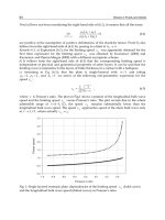
Fig. 3. In fact, cavities are modeled as parallel resonant
LC circuits in order to facilitate
discussions or analyses. The resonant frequency is inversely proportional to the square root
of inductance and capacitance;

Electromagnetic Waves in Cavity Design

81

22
000
0
11
ln
2
i
LC
rr r
h
dr
ω
εμ
==
−
.
(12)
2.4 Unloaded Q in cylindrical cavity
In the cavity undergoing free oscillations, the fields and surface currents all vary linearly
with the degree of excitation, that is, a change in one quantity is accompanied by a
proportional change in the others. The stored energy and the energy losses to the walls vary
quadratically with the degree of excitation.
Since the quality factor
Q of the resonator is the ratio of the stored energy and the energy
losses per cycle to the walls, it is independent of the degree of excitation.

loss
LI
f energy stored in the cavity
UL
Q
p
ower lost P R
RI
2
0
2
1
2( )
2
.
1
()
2
π
ωω ω
====
(13)
The resonator losses per second, besides being proportional to the degree of excitation, are
inversely proportional to the product of the effective depth of penetration of the fields and
currents into the walls, the skin depth, and the conductivity of the metal of the walls. Since
the skin depth is itself inversely proportional to the square root of the conductivity, the
losses are inversely proportional to the square root of the conductivity. The losses are also
roughly proportional to the total internal surface area of the cavity; and this area is
proportional to the square of the resonant wavelength for geometrically similar resonators.

The skin depth is proportional to the square root of the wavelength, and hence the losses per
second are proportional to the three-halves power of the resonant wavelength.
The loss per cycle, which is the quantity that enters in Q , is proportional to the five-halves
power of the resonant wavelength. Since the energy stored is roughly proportional to the
volume, or the cube of the wavelength, the Q varies as the square root of the wavelength
for geometrically similar cavities, a relationship that is exact if the mode is unchanged
because the field patterns are the same. In general, large cavities, which have large resonant
wavelengths in the principal mode, have large values of Q . Cavities that have a surface
area that is unusually high in proportion to the volume, such as reentrant cavities, have Q 's
that are lower than those of cavities having a simpler geometry.
The surface current, J , is equal in magnitude to H
φ
at the wall. The power lost is the
surface integral over the interior walls of the cavity.

0
2
2
222
0
0
2
2
00
22
2( )2 2 2
22 2 2
1
2ln ,
22

ss
loss
r
s
r
oo
s
RR
PJdsHds
RI I I
rh d rdr rh
rrr
RI h d r h
RI
rrr
φ
πππ
πππ
π
==


  
=−++


  
  





−

=++≡





(14)

Behaviour of Electromagnetic Waves in Different Media and Structures

82
where the shunt resistance is

s
Rhd r h
R
rrr
00
2ln
2
π
−


≡++





.
(15)
The surface current can be considered concentrated in a layer of resistive material of
thickness. Surface resistance is that

s
f
R
f
11
.
1
π
μ
σδ σ
σ
πμσ
== =
(16)
As an example, the conductivity of copper is
copper
m
7
5.8 10 /
σ
=× Ω and since copper is
nonmagnetic

copper
Hm
7
0
410 /
μμπ
−
==× , hence, in case of that cavity material is copper, for
f=6GHz,

s
m
R
R
LH
L
Q
R
2
3
10
0
0.85
2.02 10
2.66 10
1.01 10
1431.
δ
μ
ω

−
−
−
=
=×Ω
=×Ω
=×
==

(17)
The shunt conductance G is, as given by the expression,

ener
gy
lost
p
er ond
G
Vt
2
(sec)
()
=

(18)
is defined only when the voltage
Vt()
is specified. In a reentrant cavity the potential across
the gap varies only slightly over the gap if the gap is narrow and the rest of the cavity is not
small. A unique definition is obtained for G by using for

Vt()
the potential across the
center of the gap. The gap voltage is proportional to the degree of excitation, and hence the
shunt conductance is independent of the degree of excitation. For geometrically similar
cavities the shunt conductance varies inversely as the square root of the resonant
wavelength for the same mode of excitation. This relationship exists because for the same
excitation
Vt
2
( ) is proportional to the square of the wavelength and the loss per second to
the three-halves power of the wavelength.
2.5 Lumped-constant circuit representation
The main value of the analogy between resonators and lumped-constant circuits lies not in
the extension of characteristic parameters to other geometries, in which the analogy is not
very reliable, but in the fact that the equations for the forced excitation of resonators and
lumped-constant circuits are of the same general form.
If, for example, it is assumed that the current i(t) passes into the shunt combination of
L , C
and conductance G , by Kirchhoff's laws, (see Fig. 3)

Electromagnetic Waves in Cavity Design

83

dV t
it C Vtdt GVt
dt L
() 1
() () ().=+ +


(19)


Fig. 3. Limped-constant circuit
On taking the derivative and eliminating
L ,

2
2
0
2
() () ()
()
dit dVt Vt
CVtG
dt dt dt
ω

=++


.
(20)
In other word,

di t d V t dV t
Vt
Cd d d
2

22
0
2
() () ()
2(),
ω
ωγωω
θθ θ
=+ +

(21)
where
2GC
γ
= ,
0
1 LC
ω
= and t
θω
= , which are used to calculate numerically the
initial beam effect in the last chapter.
For a forced oscillation with the frequency
ω
,

iG
j
CV
0

0
0
ωω
ωω
ω
ωω



=+ −






.
(22)
Thus, there is defined circuit admittance

YGjC
0
0
0
ωω
ω
ωω

=+ −



.
(23)
These equations describe the excitation of the lumped-constant circuit.
3. Numerical analysis for the high frequency oscillator system with
cylindrical cavity
In this section, we will meet an circular cavity example of a klystrode as a high frequency
oscillator system with the knowledge which is described in previous sections.

Behaviour of Electromagnetic Waves in Different Media and Structures

84
Conventional klystrodes and klystrons often have toroidal resonators, i.e., reentrant cavity
with a loop or rod output coupler for power extraction. These resonators commonly use
solid-electron-beam which could limit the output power. One way to get away this
limitation is to use the annular beam as was commonly done in TWTs. The main reason
using reentrant cavities in most microwave tubes with circular cross sections is that the gap
region should produce high electric field and thus high interaction impedance of the
electron beam when the cavity is excited. In our design we assume a short cavity length,
d ,
along the longitudinal direction parallel to the electron motion. In the meantime the width
of electron beam tunnel,
i
rr
0
− , is much larger, i.e.
i
dr r
0


 − as shown in Fig 4. And thus the
efficiency of beam and RF interaction in this klystrode cavity depends sensitively upon the
cavity shape at the beam entrance of the RF cavity in the beam tunnel. A simple trade-off
study suggests to put to use of gridded plane, so-called a cavity grid (anode), so that the
eigenmode of the reentrant cavity is maintained. With the gridded plane removed and left
open, the TM01-mode has many competing modes and the interaction efficiency disappears.
The use of thin cavity grid in the beam tunnel, however, can slightly reduce the electron
beam transmission, which will not pose a much of problem when the same type of grid is
used in between the cathode and anodic cavity grid. In the simulations with the MAGIC
and HFSS codes, the anodic cavity grid could be assumed to be a smooth conducting
surface, and pre-bunched electrons were launched from those surfaces of cavity grid. This
kind of concept can provide a compact microwave source of low cost and high efficiency
that is of strong interest for industrial, home electronics and communications applications.


Fig. 4. Schematics of the annular beam klystrode with the resonator grids for the high
electric field and high interaction efficiency in the gap region. This cavity structure allows
easier power extraction through the center coax coupler
The klystrodes consist of the gated triode electron gun, the resonator and the collector. The
gated electron gun provides with the pre-modulated electron bunches at the fundamental
frequency of the input resonator, where the voltage on the grid electrode is controlled by an
external oscillator or feedback system. The other possible type of gated electron guns could

Electromagnetic Waves in Cavity Design

85
be the field-emitter-array gun, RF gun, and photocathode. The electron bunches arrive at
the output gap with constant kinetic energy but with the density pre-modulated. Here, we
assumed the electron beam is operated on class B operation, that is, electron bunch length is
equal to one half of the RF period. Through the interaction between electron beam and RF

field, the kinetic energy is extracted from the pre-modulated electrons and converted into
RF energy.
Figure 4 shows the schematics of the circular gridded resonator with center coupling
mechanism for the easy and efficient power extraction. In this section, we will describe the
design of annular beam klystrode in C-band.
3.1 RF interaction cavity design
As we have seen in previous section, using the lumped-circuit approach, the resonant
frequency of this protuberance cavity with the annular beam is expressed as


i
LC
rr r
h
dr
22
000
0
11
ln
2
ω
εμ
==
−
.
(24)
Since this expression is an approximation which gives the tendency of frequency variation
when we are adjusting design parameters, we can perform parameter tuning exercise using
design tools such as HFSS. Fig. 5 shows an example of the detailed design using HFSS

where the emission was introduced at the gap region between inner radial distances of 5.7
and 9.4mm. In the figure, the electric field is enhanced and fairly uniform due to the
presence of resonator grid1 and resonator grid2. The grid structure in beam inlet and beam
outlet make the electric field maintain fairly high intensity in the gap region through which
the electron beam passes to interact with RF. Figure 6 also show scattering parameter plots
where resonator grids of the klystrode are considered closed metal wall and the cavity has
only output terminal as one port system. The bold line is the real value of S and the thin line
is the imaginary one. The resonator frequency is 5.78 GHz in the absence of finite
conductivity of cavity and electron beam.
The detailed tuning of beam parameters for efficient klystrode could be investigated using
PIC code such as MAGIC. As an example, the current is assumed density-modulated in the
input cavity and cut-off sinusoidal,

()
()
() ()
0
0
2
0
(0,) sin ,0
11 2
sin cos 2
2(41)
n
Iz t IMAX t
It nt
n
ω
ωω

ππ
∞
−
==


=+ −


−




(25)
whose peak current, I
peak
, is 3 amperes.
The tube is supposed of being operated in class B as shown in Fig. 7. A class B amplifier is
one in which the grid bias is approximately equal to the cut-off value of the tube, so that the
plate current is approximately zero when no exciting grid potential is applied, and such
that plate current flows for approximately one-half of each cycle when an AC grid voltage is
applied.

Behaviour of Electromagnetic Waves in Different Media and Structures

86

Fig. 5. Magnitude of axial electric field and azimuthal magnetic field (in relative unit) along
the radial distance on the mid-plane between resonator grid 1 and grid 2 in the cavity.

Emission surface is between the radial distances of 5.7 and 9.4 mm


Fig. 6. Scattering parameter plots. The resonator frequency is 5.78 GHz in the absence of
finite conductivity of cavity and electron beam
Radial Distance (mm)
Axial Electric Field and Azimuthal MagneticField
(Relative Unit)
E field
H field
Real & Imaginary Components
S parameter
Frequenc
y
(GHz)

Electromagnetic Waves in Cavity Design

87

Fig. 7. Pre-modulated electron beam in current vs. time; cut-off sinusoidal current which is
used in class B operation,
()
()
IIMAX t
0
sin ,0
ω
=
The fundamental mode (TM

01
-mode) to be interacted with longitudinal traversing electron
beam was adapted to our annular beam resonators for the high efficiency device.
Electron transit angle between electrodes gives limitation in the application of the
conventional tubes at microwave frequencies. The electron transit angle is defined as

g
dv
0
,
β
ωτ ω
==
(26)
where
g
dv
0
τ
= is the transit time across the gap, d is separation between cathode and
grid,
veVm V
6
00 0
2 0.593 10==× is the velocity of the electron, and V
0
is DC voltage.


Fig. 8. Electric field in the gap region across the anode electrode 1(grid1) and electrode

2(grid2); The field reaches 4,000,000 V/m

Behaviour of Electromagnetic Waves in Different Media and Structures

88
The transit angle was chosen to give that the transit time is much smaller than the period of
oscillation for the efficient interaction between RF and electron beam, so that, the beam
coupling coefficient,
M
, is 0.987 . The resonant frequency is 5.78 GHz in cold cavity and 6.0
GHz in hot cavity. Although the frequency shift may be greater than the value of normal
case, this would be come from the fact that this annular beam covers much more area with
electron beam than the conventional solid beam in a given geometry. As we can see in Fig. 8
and Fig. 9, this resonant cavity is filled and saturated with the RF power in 50 ns, and
reveals high efficiency of about 67%. The output power is 1250 W so that the efficiency of
this annular beam klystrode reveals 67 % at 6.004 GHz.


Fig. 9. Output power going through the output port vs. time where driving frequency is
6GHz. It goes to about 1.25kW
3.2 RF interaction efficiency calculation
There are some computational design codes for the klystrode. But in this section, 1-
dimensional but realistic electron beam and electric field shape are introduced to develop
analytical calculations for the klystrode design, which results in easy formulas for the
efficiency and electric field in the gap region of the klystrode in steady state.
Maxwell's equations for electron beams are followings,
E ,
ρ
ε
∇⋅ =−

(27)

B
E
t
∂
∇× =−
∂

(28)

Electromagnetic Waves in Cavity Design

89
and

D
HJ
t
.
∂
∇× = +
∂

(29)
As an approximation, the electron dynamics is in 1-D space. Then, the Maxwell's equations
are simplified as the followings.

E
z

,
ρ
ε
∂
=−
∂

(30)

B
t
0
∂
=
∂

(31)
and

BE EdE
vv
tz tdt
0.
ρε ε ε ε
∂∂ ∂
−+ = + = =
∂∂ ∂

(32)
Therefore, this means that

E remains constant for each electrons moving with velocity,
v
.
From the Lorentz force equation,

dv e
Econst
dt m
(.)=− =

(33)
for each particle with velocity
v
.
Define the snapshot time be
τ
such that,

xy
tt,
τ
=+
(34)
where
x
t is transit time for the moving particle from resonator grid1 to the transit distance,
z
, and
y
t is leaving time for moving particle from the resonator grid1. Its definition is

shown in schematic representation for the transit time, departure time, snapshot time, and
transit distance in Fig. 10.
Therefore, we can say that the variables of electrons are denoted by

y
x
e
vv Ett
m
0
(),=−
(35)

x
y
x
e
zvt Ett
m
2
0
()
2
=−
(36)
and

()
peak
y

J
Max t
v
sin( ),0 .
ρω
=
(37)
Let’s assume that
yy
Et E t
0
() sin( )
ω
=
which is synchronous to current modulation for the
maximum interaction between electron beam and RF-field.

Behaviour of Electromagnetic Waves in Different Media and Structures

90

Fig. 10. Schematic representation for the definition of snapshot time (
τ
), transit time (
x
t ) to
z , departure time (
y
t )
Then, we have

y
x
e
vv E tt
m
00
sin( )
ω
=−
(38)
and

x
y
x
e
zvt E tt
m
2
0
sin( ) .
2
ω
=−
(39)
By the way, from the above equation,

z
x

vv
zt
0
2
+
=

(40)
and

d
d
T
vv
0
2
=
+

(41)
so that for
p
eriod ps cm( ) 167 ( 5 )
λ
==

Tpsps psps
0
15 ,30 , 0 ,167 ,
τ

∈∈

 

 

(42)
and

x
tpsps0,30 .∈





(43)

Electromagnetic Waves in Cavity Design

91
Figure 11 shows a typical case that electrons are decelerated due to the interaction
between RF and electron beam. Extreme case would be 100 % donation of its kinetic
energy to RF, which makes its velocity be zero at the resonator grid2. In that case
electrons are delayed by 30 ps to the phase of RF field, where the half period of RF is 84 ps
(6 GHz).


Fig. 11. Electrons are decelerated due to the interaction between RF and electron beam.
Extreme case would be 100% donation of its kinetic energy to RF, which makes its velocity

be zero at the resonator grid2. In that case electrons are delayed by 30ps to the phase of RF
field, where the half period of RF is 84ps (6GHz)
The resonator field theory is described by the equation

E
Eout
dU
UP
dQ
,
ω
τ
=− +
(44)
where
out
P is the energy output from the bunch and
E
U is the electric energy in the cavity.
The value of
out
P depends on the behavior of the individual electrons as they move across
the gap which in turn depends on the gap voltage and field profile. The axial electric field is
only assumed by sinusoidal shape as
yy
Et E t
0
() sin( )
ω
= .

Define

yyy
f
tftdt
2
0
() () .
2
π
ω
ω
π
≡


(45)
Then, the time-averaged output power becomes

()
()
()
dd
out peak y
d
peak
peak y y
P Evdz J E Max t dz
JEd
JE tdzdt

2
0
00
2
0
2
0
00
sin ,0
sin .
24
π
ω
ρω
ω
ω
π
==
==



(46)
Because E 0= when there are non electron charges, from the Maxwell's equation set,
to the anode electrode 2
30ps
84ps

Behaviour of Electromagnetic Waves in Different Media and Structures

92

()
()
()
() ()
dd
Ey y
d
yy
E
UEMaxtdz tdz
QQ Q
EEdEd
tdz t
QQQ
2
2
22
0
0
00
222
22
000
0
sin ,0 sin
222
sin sin .
448

ωεω εω
ωω
εω εω εω
ωω
=≅
===



(47)
Since

out E
PU
Q
ω
=
(48)
at steady state, we have

p
eak
QJ
E
0
2
.
εω
=
(49)

Therefore, the efficiency becomes that

peak
out
peak
d
peak
JEd
P
QJ d
E
J
JV V V
V
0
0
4
.
42
π
π
η
εω
π
== ==
(50)
As an example,

Fm
dm

Q
12
9
3
8.85 10 / ,
210/sec,
0.4 10 ,
37
ε
ωπ
−
−
=×
=×
=×
=

(51)
give us the followings

peak
JAcm
2
32 32
3
1.71[ / ],
{(9.4 10 ) (5.7 10 ) }
π
−−
==

×−×

(52)
where Vvolts2000= ,
eC
19
1.6 10
−
=×
, and mkg
31
9.1 10
−
=× .
Therefore,

peak
QJ d
V
0.60
2
π
η
εω
==
(53)
and

peak
QJ

EVm
6
0
2
3.8 10 / .
εω
==×
(54)
In the previous example, we have seen that the tube reveals 67% efficiency and the electric
field in the gap region was Vm
9
410 /× . This result of the numerical analysis is well
matched with the above theoretical calculations.

Electromagnetic Waves in Cavity Design

93
On the other hand, we can compare MAGIC analysis with analytical calculation as can be
seen Fig. 12 which shows efficiency vs. peak current density by MAGIC PIC simulation and
analytical calculation. The slope of the line fitted with the results from MAGIC analysis
shows 0.266.
From the analytical equation of efficiency, we can get the slope of the line, m, as the
followings,

peak
Qd
mcmA
JV
2
0.348 / .

2
ηπ
εω
== =
(55)
Analytical calculation says the slope of the line be 0.348 . MAGIC and analytical equation
reveal that as we increase the current density, the efficiency of the tube also increases.


Fig. 12. Efficiency vs. peak current density. Square dots are results from MAGIC simulation.
Solid line is line fit with the results. Dotted line is analytical calculation. The slope of the
solid line, line fit with the MAGIC results, is 0.266 and that of dotted line from analytical
calculation is 0.348
4. Cavity design for the uniform atmospheric microwave plasma source
The atmospheric-pressure microwave-sustained plasma has aroused considerable interest
for many application areas. The advantages of this plasma are electrode-less operation and
efficient microwave-to-plasma coupling. It has the characteristics of high plasma density
( cm
13 3
10 /
−
≈ ) and efficient energy conversion from microwaves to the discharged plasma
which is high-efficient plasma discharge (~80%). An atmospheric-pressure microwave-
sustained plasma can be formed in a rectangular resonant cavity, a waveguide, or a surface-

Behaviour of Electromagnetic Waves in Different Media and Structures

94
effect system. This plasma has been widely used in the laboratory spectroscopic analysis,
continuous emissions monitoring in the field, commercial processing, and other

environmental applications.
Atmospheric-pressure microwave plasma sources consist of a magnetron as a microwave
source, an isolator to isolate the magnetron from the harmful reflected microwave, a
directional coupler to monitor the reflected microwave power, a 3-stub tuner to match
impedance from the magnetron to that from the plasma generator, and a plasma generator
through which gases pass and are discharged by the injected microwave. The plasma in the
discharge generator is sustained in a fused quartz tube which penetrates perpendicularly
through the wide walls of a tapered and shorted WR-284 waveguide.
The plasma’s cross-sectional area of the atmospheric-pressure microwave plasma source is
limited by the quartz tube’s diameter, which is also limited by the maximum intensity of the
electric field profile sustainable by the injected microwave and the shorted waveguide
structure, as shown in the Fig. 13. The diameter of the quartz tube is set around 30 mm to
maintain a dischargeable electric field intensity in the discharge area. If the diameter of the
quartz tube becomes much larger than that, no discharge occurs. This is the main reason
that the cross-sectional area cannot be extended more widely in the atmospheric-pressure
microwave-sustained plasma source.


Fig. 13. Schematic illustrations of the atmospheric pressure microwave plasma source using
a quartz tube located a quarter wavelength from the end of the shorted waveguide to
maintain a high electric field intensity to discharge the passing- gases to generate a plasma
efficiently
Here is an example of a rectangular reentrant resonator, a single ridge cavity, to overcome
this size-limited plasma discharge in an atmospheric microwave-sustained plasma source.
The box-type 915 MHz reentrant resonator has gridded walls on both sides of the gap so
that the plasma gases pass thorough the grid holes and are discharged by the induced

Electromagnetic Waves in Cavity Design

95

electric gap field due to the injected microwave energy. As we have studied in last section,
it could be calculated analytically the cavity design formula by using lumped-circuit
approximation, then, we performed a RF simulation by using the HFSS (High Frequency
Structure Simulator) code. The designed plasma cross-sectional area is 810 mm x5 mm.
The cavity has a fundamental TE
10
-like mode to discharge gases uniformly between the
gridded walls and has a 915 MHz resonant frequency. This large cross-sectional area
plasma torch can be effectively used in commercial processing and other environmental
applications.
4.1 Numerical analysis of the plasma source rectangular cavity
A reentrant cavity in cylindrical symmetry has been widely used in vacuum tubes such as
klystrodes and klystrons. However, in order to keep the resonant frequency constant
whatever the cavity lengths for atmospheric microwave plasma torch, it would be better to
consider a rectangular reentrant cavity, as shown in Fig. 14. The resonant frequency of the
cavity for the atmospheric microwave plasma source has a fundamental TE
10
-like mode.


Fig. 14. Schematic of the box-type resonator cavity as a atmospheric pressure microwave
plasma source with grids to maintain a high electric field intensity to discharge the passing
gases to generate plasma efficiently in the gap region
The gap region between the two gridded walls in the reentrant cavity sustains a high electric
field intensity and, thus, easily discharges the gases to the plasma state when it is excited by
the microwave energy. With the grid planes surrounding the gap region, the TE
10
-like mode
is the dominant one, and 915 MHz is the cavity’s resonant frequency. In the simulation
process using the HFSS code, the cavity grids were assumed to be smooth conducting

surfaces to design the box-type reentrant cavity.
In this example, the cavity for the microwave plasma source was set to be resonated at 915
MHz, rather than 2.45 GHz, so as to have a much larger cross-sectional plasma area. Its
design, setting a cavity to 915 MHz, is based on the design formula obtained by using a
theoretical calculation based on the lumped-circuit approximation for the cavity. Then, we
used a simulation tool, the HFSS code, to check the cavity frequency.

Behaviour of Electromagnetic Waves in Different Media and Structures

96
From Gauss’ law, the equivalent capacitance value of the reentrant cavity for a TE
10
-like
mode is

QQ Lw
C
V EHh Hh
0
()
ε
⊥
== =
−−
, (56)
where Q , V , and E
⊥
are the stored electric charges on the grid surfaces, the electric voltage
difference, and the perpendicular electric field intensity between the opposite grid surfaces
respectively, and w ,

H , and h are designated dimensional parameters, as shown in Fig.
14. From Ampere’s law, the equivalent inductance value of the reentrant cavity for a TE
10
-
like mode can be expressed as follows. Since the magnetic field flux density in the cavity is
BIL
0
2
μ
= , and since the total magnetic flux in the box-type reentrant cavity is
BH W w()Φ= − , from the inductance definition,

HW w
L
L
0
()
4
μ
−
=
. (57)
Therefore, the cavity resonant frequency is given by

cHh
f
Hw W w()
π
−
=

−
. (58)
This resonant frequency formula shows that the resonant frequency is independent of the
cavity length
L , which means that if we extrude the plasma through this grid planes, the
plasma’s cross-sectional area can be uniformly extended as much as we want without any
influence on the cavity resonant frequency. However, because we use an available
microwave source, which has a limited RF power, to discharge the gases, the cavity length
cannot be extended to an unlimited extent. We will discuss this relationship between the
consumption RF power and the cavity length in the next paragraph.
Since we have a theoretically-approximated expression for the design parameters, we
should use this formula to pick up the initial design parameters to get detailed parameters
for the resonator reentrant cavity as a plasma source. Then we should investigate the RF
characteristics using the design tool, HFSS.
The energy stored in the gap region can be expressed as
UCV
2
1
2
=
, (59)
where C and V are the equivalent capacitance value of the cavity and the induced gap
peak voltage between the grid planes, respectively. If we assume that all of this stored
energy can be delivered to the gas discharge reaction process to generate the plasma, the
microwave power consumption can be expressed as

LV
PfCV
HH h W w
2

0
2
0
1
22()()
εω
πμ
==
−−
. (60)

Electromagnetic Waves in Cavity Design

97
In other words, the cavity length for the atmospheric-pressure microwave-sustained plasma
source is

PHHhWw
L
Vw
0
2
2000 ( )( )
πμ
−−
=
, (61)
where
V is in kV,
P

is in kW, and the dimensional parameters,
L
,
H
, h , W , and w , are
in
mm units in this formula.
Fig. 15 and Fig. 16. show a rectangular cavity design example using one of the available
magnetrons, 915 MHz, 60 kW, as a RF source, and the geometrical parameters to
Hmm29= ,
Hh mm1−= , and Wmm80= . Furthermore, if the gap voltage is the upper-limit RF air
breakdown voltage, that is, the DC breakdown voltage for air at the level of
kV cm33 / at
atmospheric pressure, the cavity length is limited by
mm810 for self discharge. In this case,
the plasma’s cross-sectional area is uniformly distributed within
mm mm810 5× , i.e.,
wmm5= .
This uniformly distributed plasma area is
mm mm810 5× , which is much larger than the
areas of the conventional atmospheric-pressure microwave-sustained plasma sources. This
large-sized microwave plasma at atmospheric pressure can be used in commercial
processing and other environmental applications area.


Fig. 15. Electric field intensity profile of the TE10-like mode from the HFSS simulation on the
mid-plane between the grid surfaces in the gap region. Both ends are shorted walls, and the
electric field profiles are distributed within
mm mm810 5× in the gap region. Microwave
energy is feeding through the coaxial coupler to the cavity. If we use a pair of these cavities

in parallel, the crest of one will compensate for the other’s trough electric field intensity
areas, which could result in a uniform microwave plasma source

Behaviour of Electromagnetic Waves in Different Media and Structures

98

Fig. 16. Scattering parameters of the box-type reentrant cavity. The solid red and dashed
blue lines are the real and imaginary values of S11, respectively. This shows that the cavity
has a resonant frequency of 904 MHz and a high Q value of 7400
5. Conclusion
The annular beam cavity design was investigated analytically and simulated using the HFSS
and MAGIC PIC codes to find the fine-tuned design parameters and optimum efficiency of
the TM
01
-mode operation in the klystrode with the reentrant interaction cavity. We also
studied how to induce the governing efficiency formular for the microwave vacuum tube,
klystrode. The efficiency of this exampled annular beam klystrode reveals 67 % at 6.004
GHz. The theoretical calculation anticipated that the efficiency would be 60% and the
electric field intensity 4000V/m which is well matched with the results of numerical
analysis. This concept could yield an economic sized device comparable to commercial
magnetron devices.
A single ridge cavity was designed to show how to design uniform atmospheric microwave
plasma source which does not need ignitors for the initial discharge. The single ridge cavity
in the shape of resonator was built in the grid structures for the wide cavity torch of
atmospheric pressure microwave plasma. This cavity design process has been studied by
analytical calculation using lumped circuit approximation and simulation using
commercial 3D HFSS code. A self-dischargeable study also has been investigated for the
breakdown feasibility in the cavity gap region. These cavities show the uniform
electromagnetic wave distribution between the grids through which large-sized microwave

plasma could be generated.
6. References
Ansoft Co. (1999). High Frequency Structure Simulator, version 6.0, Ansoft Co., PA, USA,
1999

Electromagnetic Waves in Cavity Design

99
Burton, A. J.; & Miller, G. F. (1971). The application of integral equation methods to the
numerical solution of some exterior boundary-value problems,
Proc. Roy. Soc. Lond.,
A. 323, 201 1971
Curnow, H. J. (1965). A General Equivalent Circuit for Coupled-Cavity Slowe-Wave
Structures,
IEEE Transactions on Microwave Theory and Techniques, Vol. MTT-13, No.
5, 671, Sep. 1965
Dai, F. & Omar, A. S. (1993). Field-analysis model for predicting dispersion property of
coupled-cavity circuits,
IEEE MTT-S Digest, 901 1993
Fallgatter, K.; Svoboda, V. & Winefordner, J.D. (1971). Physical and analytical aspects of a
microwave excited plasma,
Applied Spectrocopy, 25, no.3, 347 1971
Fujisawa, K. Fujisawa (1951). Theory of slotted cylindrical cavities with transverse electric
field,
Tech. Reps. Osaka Univ., Vol. 1, 69, 1951
Fujisawa,. K. (1958). General treatment of klystron resonant cavities,
IRE Trans., MTT-6, 344,
Oct. 1958
Gilmour, Jr.,A.S. (1986) Microwave Tube,
Artech House, Chap. 15 1986

Goplen, B.; Ludeking, L.; Nguyen, K. & Warren, G. (1990). Design of an 850MHz klystrode,
International Electron Devices Meeting, 889 1990
Goplen, B.; Ludeking, L.; Smithe, D. & Warren, G. (1994). MAGIC User's Manual, Rep.
MRC/WDC-R-326,
Mission Res. Corp., Newington, VA, 1994
Hamilton, D. R.; Knipp, J. K. & Kuper, J. B. Horner (1966). Klystrons and Microwave
Triodes,
Dover Pub., New York, 1966
Hansen, W. W. (1938). A type of electrical resonator,
Journal of Applied Physics, Vol. 9, 654,
Oct. 1938
HeBe, Z. (1997). The cold quality Qcold for magnicon on resonator in the rotating TMn10
mode,
International Journal of Infrared and Millimeter Waves, Vol. 18, No. 2, 437 1997
Kim, Hyoung S. & Uhm, Han S. (2001). Analytical Calculations and Comparison with
Numerical Data for Annular Klystrode,
IEEE Transactions on Plasma Science, Vol. 29,
Issue 6, pp. 875-880, Dec. 2001
Kim, Hyoung Suk & Ahn, Saeyoung (2000). Numerical Analysis of C-band Klystrode with
Annular Electron Beam,
International Journal of Infrared and Millimeter Waves, Vol. 21,
No. 1, pp. 11-20, Jan. 2000
Kleinman, R. E. & Roach, G. F. (1974). Boundary Integral equations for the three-
dimensional Helmholtz equation,
SIAM Review, Vol. 16, No. 2, 214, April 1974
Lee, S. W.; Kang, H. J.; Kim, H. S. & Hum, H. S. (2009). Numerical Design of the Cavity for
the Uniform Atmospheric Microwave Plasma Source,
Journal of Korean Physical
Society
, Vol. 54, No. 6, pp. 2297-2301, June 2009

Liao, Samuel Y. (1990). Microwave Devices & Circuits,
Prentice Hall, 1990
Marks, R. B. (1986). Application of the singular function expansion to an integral equation
for scattering,
IEEE Transactions on Antennas and Propagation, Vol. AP-34, No. 5, 725,
May 1986
Mcdonald, S. W.; Finn, J. M.; Read, M. E. & Manheimer, W. M. (1986). Boundary integral
method for computing eigenfunctions in slotted gyrotron cavities of arbitrary cross-
sections,
Int. J. Electronics, Vol. 61, No. 6, 795, 1986
Pearson, L. W. Pearson, (1984). A Note on the representation of scattered fields as a
singularity expansion,
IEEE Transactions on Antennas and Propagation, Vol. AP-32,
No. 5, 520, May 1984

Behaviour of Electromagnetic Waves in Different Media and Structures

100
Ramm, A. G. (1982). Mathematical foundations of the singularity and eigenmode expansion
methods,
Journal of Mathematical Analysis and Applications, 86, 562 1982
Riddell, R. J. Jr. (1979). Boundary-Distribution Solution of The Helmholtz Equation for a
Region with Corners,
Journal of Computational Physics, 31, 21 1979
Riekmann, C.; Jostingmeier, A. & Omar, A. S. (1996). Application of the eigenmode
transformation technique for the analysis of planar transmission lines,
IEEE MTT-S
Digest
, 1023 1996
Samuel Seely, (1950). Electron-Tube Circuits,

McGraw Hill Book Com. Inc., New York, 1950
Stevenson, A. F. (1948). Theory of slots in rectangular wave-guides,
Journal of Applied Physics,
Vol. 19, 24, Jan. 1948
Tan, J. & Pan, G. (1996). A general functional analysis to dispersive structures,
IEEE MTT-S
Digest
, 1027 1996
Tobocman, W. (1984). Calculation of acoustic wave scattering by means of the Helmholtz
integral equation. I,
J. Acoust. Soc. Am., 76 (2), 599, Aug. 1984
Zander, A.T. & Hieftje, G.M. (1981). Microwave-supported discharges,
Applied Spectroscopy,
35, no. 4, 357 1981
6
Wide-band Rock and Ore Samples Complex
Permittivity Measurement
Sixin Liu
1
, Junjun Wu
1
, Lili Zhang
2
and Hang Dong
3

1
Jilin University,
2
Shenyang Aerospace University,

3
Northeast Institute of Geography and Agroecology, CAS
China
1. Introduction
Ground penetrating radar (GPR) is based on high-frequency electromagnetic wave
propagation and its detecting targets are below the ground surface (Daniels, 2004; Jol, 2009).
Velocity and attenuation are two important factors describing the electromagnetic wave in
the media composed of rocks or soils. Velocity is inverse proportional to the root of the
permittivity while other parameters are fixed generally. In order to understand the
performance of GPR, permittivity testing and analysis are critical. In addition, during the
metal ore exploration by borehole radar which is an operating mode of GPR, the
permittivity difference between ore body and surrounding rock is the foundation for
exploration. As the sampling site, geological environment, and seasons are changing, the
permittivity are different even for the same rock. Therefore, permittivity measurement is
very important.
Currently, measurement methods are basically indirect methods which are based on
transmission line theory, characteristic impedance, and propagation constant. These
variables have intrinsic relationship with permittivity which can be inverted from the
measured data by certain calculation procedure. At the RF frequency band, common
measurement methods include short-circuited wave-guide measurement, coaxial line
transmission/reflection method, open-ended coaxial probe, resonant cavity method, free-
space transmission technique, parallel-plate capacitance method, etc.
Roberts and von Hippel (1946) developed the short-circuited wave-guide measurement,
sample is inserted at the end of the wave-guide or coaxial line, the standing wave is formed
as the incident wave and the reflected wave coexist in the wave-guide. The sanding wave
ratios (SWR’s) were required to measure in the case with and without sample. Permittivity
can be determined by the change in the widths of nodes, sample length, and the waveguide
dimension.
Resonant cavity method is a perturbation technique, which is frequently used for measuring
permittivity because of its simplicity, accuracy, and high temperature capability (Venkatesh

& Raghavan, 2005). This technique is based on the resonant frequency shift, and the change
in absorption characteristics due to the insertion of sample material. The measurement is
made by placing a sample completely in the center of a waveguide. The size of the cavity is