Waves in fluids and solids Part 4 docx

Waves in Fluids and Solids

64
Proof a) flows out from considering the right-hand-side of (6.1), it ensures that all the terms




1, ,
0
2
kk k
kn
kk k
k
 
 





(6.4)
are positive at the assumption of positive definiteness of the elasticity tensor. Proof
b) also
follows from the right-hand-side of (6.1) by passing to a limit at
n
h .
Remarks 6.1. a) Expression (6.1)
1

for the limiting speed
1
s
c was apparently obtained for the
first time; expression for the limiting speed
2
s
c was obtained by Kuznetsov (2006) and
Kuznetsov and Djeran-Maigre (2008) with a different asymptotic scheme.
b) It follows from the right-hand side of (6.3) that the corresponding limiting speed is
independent of physical and geometrical properties of other layers. It can be said that the
limiting wave is insensitive to the layers of finite thickness in a contact with a halfspace.
c) Assuming in Eq. (6.1)
1
that the plate is single-layered with 1n

and taking
11
1, 1


, and
1
1h

we arrive at the following one-parametric expression for the
speed
1
s
c :

1
11
1
2
s
c



, (6.5)
where

is Poisson’s ratio. The plot on Fig.1 shows variation of the longitudinal bulk wave
speed and the limiting speed
1
s
c versus Poisson’s ratio. The plot reveals that in the whole
admissible range of


1
2
1;

 , the speed
1
s
c remains substantially lower than the
longitudinal bulk wave speed. The speed

1
s
c approaches speed of the shear bulk wave only
at
1/2

 , where actually
1
sS
c с

.


Fig. 1. Single layered isotropic plate: dependencies of the limiting speed
1
s
c (bold curve)
and the longitudinal bulk wave speed (dotted curve) on Poisson’s ratio.

Soliton-Like Lamb Waves in Layered Media

65
d) For a triple-layered plate with the outer layers of the same physical and geometrical
properties (such a case often occurs in practice) the limiting speed
1
s
c is



1
11 22
11 22 11 22
11 22
22 /2
22
s
ch h hh
 
 
 


 



(6.6)
and
2
s
c is

2
11 22
11 22
2
2
s
hh

c
hh





, (6.7)
where index 1 is referred to the outer layers, and 2 corresponds to the inner layer. Assuming
in Eq. (6.7) that
12
hh , while other physical properties of the layers have comparable
values, yields coincidence of
2
s
c with the shear bulk wave speed of the inner layer.
Remarks 6.2. a) Expression (6.1)
1
for the limiting speed
1
s
c was apparently obtained for the
first time; expression for the limiting speed
2
s
c was obtained by Kuznetsov (2006) and
Kuznetsov and Djeran-Maigre (2008) with a different asymptotic scheme.
7. Acknowledgements
Authors thank INSA de Lyon (France) and the Russian Foundation for Basic Research
(Grants 08-08-00855 and 09-01-12063) for partial financial support.

8. References
Achenbach J.D. Wave Propagation in Elastic Solids, North-Holland Publ., Amsterdam -
London, 1973.
Arnol'd V.I. Mathematical Methods of Classical Mechanics, Springer-Verlag, N.Y., 1989.
Auld B.A. Acoustic Fields and waves in Solids, Vol.2, 2
nd
edition, Krieger Pub Co, Malabar
FL, 1990.
Barber J.R. Three-dimensional elasticity solutions for isotropic and generally anisotropic
bodies, Applied Mechanics and Materials, 5-6 (2006) 541-550.
Barber J.R. and Ting T.C.T. Three-dimensional solutions for general anisotropy, J. Mech. Phys.
Solids, 55 (2007) 1993 - 2006
Chree C. The equations of an isotropic elastic solid in polar and cylindrical coordinates, their
solutions and applications, Trans. Camb. phil. Soc. Math. Phys. Sci., 14 (1889) 250.
Craik A.D.D. The origins of water wave theory, Annual Review of Fluid Mechanics 36 (2004)
1 – 28.
Davies R. M. A critical study of the Hopkinson pressure bar, Phil. Trans. R. Soc. A240 (1948)
375 – 457.
Eckl C., Kovalev A.S., Mayer A.P., Lomonosov A.M., and Hess P. Solitory surface acoustic
waves, Physical Rev., E70 (2004) 1 - 15.
Ewing W.M., Jardetzky W.S., and Press F. Elastic Waves in Layered Media, McGraw-Hill Inc.,
N.Y., 1957.
Fu Y.B. Hamiltonian interpretation of the Stroh formalism in anisotropic elasticity, Proc.
Roy. Soc. A. 463 (2007) 3073 – 3087.

Waves in Fluids and Solids

66
Gogoladze V.G. Dispersion of Rayleigh Waves in a Layer (in Russian), Publ. Inst. Seism.
Acad. Sci. U.R.S.S. 119 (1947) 27 – 38.

Graff K. F. Wave Motion in Elastic Solids, Dover Inc., N.Y., 1975.
Hartman P. Ordinary differential equations, John Wiley & Sons, Inc., N.Y., 1964.
Haskell N.A. Dispersion of surface waves on multilayered media, Bull. Seismol. Soc.
America. 43 (1953) 17 – 34.
Higham N. J. Evaluating Padé approximants of the matrix logarithm, SIAM J. Matrix Anal.
Appl., 22 (2001) 1126 – 1135.
Holden A.N. Longitudinal modes of elastic waves in isotropic cylinders and slabs, Bell Sys.
Tech. J. 30 (1951) 956 – 969.
Kaplunov J.D. and Nolde, E.V. Long-Wave Vibrations of a Nearly Incompressible Isotropic
Plate with Fixed Faces, Quart. J. Mech. Appl. Math. 55 (2002): 345 – 356.
Kawahara T. Oscillatory solitary waves in dispersive media, J. Phys. Soc. Japan 33 (1972) 260
– 268.
Kliakhandler I.L., Porubov A.V., and Velarde M.G. Localized finite-amplitude disturbances and
selection of solitary waves, Physical Review E 62 (2000) 4959-4962.
Korteweg D.J. and de Vries F. On the Change of Form of Long Waves Advancing in a
Rectangular Canal, and on a New Type of Long Stationary Waves, Philosophical
Magazine 39 (1895) 422 – 443.
Knopoff L. A matrix method for elastic wave problems, Bull. Seismol. Soc. Am. 54 (1964) 431
– 438.
Kuznetsov S.V. Subsonic Lamb waves in anisotropic plates, Quart. Appl. Math. 60 (2002) 577
– 587.
Kuznetsov S.V. Surface waves of non-Rayleigh type, Quart. Appl. Math. 61 (2003) 575 – 582.
Kuznetsov S.V. SH-waves in laminated plates, Quart. Appl. Math., 64 (2006) 153 – 165.
Kuznetsov S.V. and Djeran-Maigre I., Solitary SH waves in two layered traction free plates,
Comptes Rendus Acad Sci., Paris, Ser. Mecanique, №336(2008) pp. 102 – 107.
Lamb H. On waves in an elastic plate, Proc. Roy. Soc. A93 (1917) 114 – 128.
Lange J.N. Mode conversion in the long-wavelength limit, J. Acoust. Soc. Am., 41 (1967)
1449-1452.
Lax P. Integrals of Nonlinear Evolution Equations and Solitary Waves, Comm. Pure Appl.
Math. 21 (1968) 467 – 490.

Lekhnitskii S.G. Theory of Elasticity of an Anisotropic Elastic Body. Holden-Day, San
Francisco 1963.
Li, X D., and Romanowicz B. Comparison of global waveform inversions with and without
considering cross-branch modal coupling, Geophys. J. Int., 121 (1995) 695 – 709.
Lowe M.J.S. Matrix techniques for modeling ultrasonic waves in multilayered media, IEEE
Transactions on Ultrasonics, Ferroelectrics, and Frequency Control 42 (1995) 525 –
542.
Lowe M.J.S. A computer model to study the properties of guided waves., J. Acoust. Soc. Am.,
123 (2008) 3654 – 3654.
Lyon R.H. Response of an elastic plate to localized driving forces, J. Acoust. Soc. Am., 27
(1955) 259 – 265.
Mal A.K., Knopoff L. A differential equation for surface waves in layers with varying
thickness, J. Math. Anal. Appl. 21 (1968) 431 – 441.

Soliton-Like Lamb Waves in Layered Media

67
Meeker T.R. and Meitzler A.H. Guided wave propagation in elongated cylinders and plates,
in: Physical Acoustics, (Ed. W. P. Mason) Vol. 1, Part A, Chap. 2. Academic Press,
New York 1964.
Meyer C.D. Matrix Analysis and Applied Linear Algebra, SIAM, N.Y., 2002.
Miles J.W. The Korteweg-de Vries equation, a historical essay, J. Fluid Mech. 106 (1981) 131 –
147.
Miklowitz J. Elastic waves and waveguides, North-Holland, Amsterdam, 1978.
Mindlin R.D. The thickness shear and flexural vibrations of crystal plates. J. Appl. Phys. 22
(1951) 316.
Mindlin R.D. Influence of rotatory inertia and shear on flexural motions of isotropic, elastic
plates, J. Appl. Mech., 18 (1951) 316.
Mindlin R.D. Vibrations of an infinite elastic plate and its cut-off frequencies, Proc Third US
Nat. Congr. Appl. Mech., (1958) 225.

Mindlin R.D. Waves and vibrations in isotropic, elastic plates. In Structural Mechanics
(Editors J.N. Goodier and N. Hoff). (1960) 199 – 232.
Mindlin R.D. and McNiven H.D. Axially symmetric waves in elastic rods, J. Appl. Mech., 27
(1960) 145 – 151.
Mindlin R.D. and Medick M.A. Extensional vibrations of elastic plates, J. Appl. Mech., 26
(1959) 561 – 569.
Mindlin R.D. and Onoe M. Mathematical theory of vibrations of elastic plates, In:
Proceedings of the XI Annual Symposium on Frequency Control U. S. Army Signal
Corps Engineering Laboratories, Fort Monmouth, New Jersey (1957) 17 – 40.
Moler C. and Van Loan Ch. Nineteen Dubious Ways to Compute the Exponential of a Matrix,
SIAM Review, 20 (1978) 801 – 836.
Moler C. and Van Loan Ch. Nineteen Dubious Ways to Compute the Exponential of a Matrix,
Twenty-Five Years Later SIAM Review, 45 (2003) 3 – 48.
Onoe M. A study of the branches of the velocity-dispersion equations of elastic plates and
rods, Report: Joint Commitee on Ultrasonics of the Institute of Electrical
Communication Engineers and the Acoustical Society of Japan, (1955) 1 – 21.
Onoe M., McNiven H.D., and Mindlin R.D. Dispersion of axially symmetric waves in elastic
rods, J. Appl. Mech., 29 (1962) 729 – 734.
Pagneux V., Maurel A. Determination of Lamb mode eigenvalues, J. Acoust. Soc. Am., 110(3)
(2001) Sep.
Planat M., Hoummady M. Observation of soliton-like envelope modulation generated in an
anisotropic quartz plate by metallic in interdigital transducers, Appl. Phys. Lett, 55
(1989) 103 – 114.
Pochhammer L. Uber die Fortpflanzungsgeschwindigkeiten kleiner Schwingungen in einem
unbegrenzten istropen Kreiszylinder, J. reine angew. Math. 81 (1876) 324 – 336.
Poncelet O., Shuvalov A.L., and Kaplunov J.D. Approximation of the flexural velocity branch in
plates, Int. J. Solid Struct., 43 (2006) 6329 – 6346.
Porubov I.V., Samsonov A.M., Velarde M.G., and Bukhanovsky A.V. Strain solitary waves in an
elastic rod embedded in another elastic external medium with sliding, Phys.Rev.
Ser. E, 58 (1998) 3854 – 3864.

Russell Scott J. Report on waves, In: Fourteenth meeting of the British Association for the
Advancement of Science, York, 1844 (London 1845), 311 – 390.

Waves in Fluids and Solids

68
Ryden N., Lowe M.J.S., Cawley P., and Park C.B. Evaluation of multilayered pavement
structures from measurements of surface waves, Review of Progress in
Quantitative Nondestructive Evaluation, 820 (2006) 1616 – 1623.
Simonetti F. Sound Propagation in Lossless Waveguides Coated with Attenuative Materials,
PhD thesis, Imperial Colledge, 2003.
Soerensen M.P., Christiansen P.L., and Lomdahl P.S. Solitary waves on nonlinear elastic rods. I.
J. Acoust. Soc. Amer., 76 (1984) 871 – 879.
Stroh A.N. Dislocations and cracks in anisotropic elasticity. Phil. Mag. 3 (1958) 625-646.
Stroh A.N. Steady state problems in anisotropic elasticity, J. Math. Phys. 41 (1962) 77 - 103.
Tanuma K. Stroh Formalism and Rayleigh Waves (Reprinted from J. Elasticity, 89, 2007),
Springer, N.Y., 2007.
Tarn J Q. A state space formalism for anisotropic elasticity. Part. I. Rectilinear anisotropy.
Int. J. Solids Structures, 39 (2002) 5157 – 5172.
Tarn J Q. A state space formalism for anisotropic elasticity. Part. II. Cylindrical anisotropy.
Int. J. Solids Structures, 39 (2002) 5143 – 5155.
Thomson W.T. Transmission of elastic waves through a stratified solid medium, J. Appl.
Phys. 21 (1950) 89 – 93.
Ting T.C.T. Anisotropic elasticity: theory and applications. Oxford University Press, New
York, 1996.
Ting T.C.T. A modified Lekhnitskii formalism á la Stroh for anisotropic elasticity and
classifications of the 6X6 matrix N, Proc. Roy. Soc. London, A455 (1999) 69 – 89.
Ting T.C.T. Recent developments in anisotropic elasticity. Int. J. Solids Structures, 37 (2000)
401 – 409.
Ting T.C.T. and Barnett D.M. Classifications of surface waves in anisotropic elastic materials.

Wave Motion 26 (1997) 207 – 218.
Tolstoy I. and Usdin E. Dispersive properties of stratified elastic and liquid media: a ray
theory. Geophysics 18 (1953) 844 – 870.
Treves F. Introduction to Pseudodifferential and Fourier Integral Operators, Vol.1, Plenum
Press, N.Y. and London, 1982.
Yan-ze Peng Exact periodic wave solutions to a new Hamiltonian amplitude equation, J.
Phys. Soc. Japan 72 (2003) 1356 – 1359.

Zanna A.
and Munthe-Kaas H.Z. Generalized polar decompositions for the approximation of
the matrix exponential, SIAM J. Matrix Anal. Appl., 23 (2002) 840 – 862.
Zwillinger D. Handbook of Differential Equations, Academic Press, Third Edition, 1998.
3
Surface and Bulk Acoustic
Waves in Multilayer Structures
V. I. Cherednick and M. Y. Dvoesherstov
Nizhny Novgorod State University
Russia
1. Introduction
The application of various layers on a piezoelectric substrate is a way of improving the
parameters of propagating electroacoustic waves. For example, a metal film of certain
thickness may provide the thermal stability of the wave for substrate cuts, corresponding to
a high electromechanical coupling coefficient. The overlayer can vary the wave propagation
velocity and, hence, the operating frequency of a device. The effect of the environment (gas
or liquid) on the properties of the wave in the layered structure is used in sensors. The layer
may protect the piezoelectric substrate against undesired external impacts. Multilayer
compositions allow to reduce a velocity dispersion, which is observed in single-layer
structures. In multilayer film bulk acoustic wave resonators (FBAR) many layers are
necessary for proper work of such devices. Therefore, analysis and optimization of the wave
propagation characteristics in multilayer structures seems to be topical. General methods of

numerical calculations of the surface and bulk acoustic wave parameters in arbitrary
multilayer structures are described in this chapter.
2. Surface acoustic waves in multilayer structures
In the linear theory of piezoelectricity and in the quasistatic electric approximation the
system of differential equations, describing the mechanical displacements u
i
along the three
spatial coordinates x
i
(i = 1, 2, 3) and the electric potential

in the solid piezoelectric
medium, may be written in such view (Campbell and Jones, 1968):

2
2
2
2
j
k
ijkl kij
il ki
u
u
ce
xx xx
t







 

(1)

2
2
0
k
ikl ik
il ik
u
e
xx xx






 
i, j, k, l = 1, 2, 3 (2)
In these equations
c
ijkl
is the forth rank tensor of the elastic stiffness constants, e
ijk
is the third

rank tensor of the piezoelectric constants,


ij
is the second rank tensor of the dielectric
constants,

- the mass density, t – time, and the summation convention for repeated indices
is used. The expression (1) contains three equations and (2) gives one more equation, totally

Waves in Fluids and Solids

70
four equations. These equations must be solved for each medium of all the multilayer
system, which is shown in Fig. 1.


Fig. 1. Multilayer structure - substrate and M layers.
The coordinate axis
x
1
direction coincides with the wave phase velocity v, the coordinate
axis x
3
is normal to the substrate surface and the axis origin is set on this surface, as shown
in Fig 1. A solution of equations (1) and (2) we will seek in the following form:
exp[ ( )]
jj ii
uikbxvt




4
exp[ ( )]
ii
ik b x vt


Here

j
– amplitudes of the mechanical displacements,

4
– the amplitude of the electric
potential, b
i
– directional cosines of the wave velocity vector along the corresponding axises,
k =

/v = 2/

– the wave number,

– a circular frequency,

– a wavelength. Substitution
of (3) into (1) and (2) gives the system of four linear algebraic equations for wave
amplitudes:

2
4i
j
kl i l k ki
j
ki
j
cbb ebb v


 (4)

4
0
ikl i l k ik i k
ebb bb
 

 (5)
The detailed form of these equations is following:

2
11 1 122 133 144
2
21 1 22 2 23 3 24 4
2
31 1 32 2 33 3 34 4
41 1 42 2 43 3 44 4
() 0
() 0

() 0
0
v
v
v
   



    



(6)
Here:

44 44
, , , , , 1,2,3
jk kj ijkl i l j j ikj i k ik i k
cbb ebb bb ijkl

   
(7)
For the existence of a nontrivial solution of the system (6) a determinant of this system must
be equal to zero:
Layer
1

0
h

1

h
2

h
M


x
3

Layer
M

Layer
2

Substrate

x
1

i, j

= 1, 2, 3 (3)


Surface and Bulk Acoustic Waves in Multilayer Structures

71

2
11 12 13 14
2
21 22 23 24
2
31 32 33 34
41 42 43 44
0
v
v
v



   
 



(8)
This equation allows to determine the unknown directional cosine b
3
, if the values v, b
1
, and
b
2
are set. For flat pseudo-surface acoustic wave the values of the directional cosines are

following:

123
1, 0,bib bb


, (9)
where

is the wave attenuation coefficient along the propagation direction. For surface
acoustic wave the attenuation is absent and

= 0. The equation (8) with taking into account
(9) gives the following eighth power polynomial equation with respect to the b value:

8765432
876 54 32 10
0ab ab ab ab ab ab ab ab a

 (10)
Coefficients a
i
of this equation are represented by very complicated expressions, depending
on material constants of the medium, a phase velocity v, and the attenuation coefficient

.
For pseudo-surface acoustic waves

≠ 0 and therefore coefficients a
i

are complex values. For
surface acoustic waves

= 0 and coefficients a
i
are pure real values. In this case roots of the
equation (10) are either real or complex conjugated pairs. If

≠ 0, roots of the equation (10)
are complex but not conjugated. So, solving (numerically certainly) the equation (10), we get
eight roots b
(n)
(n = 1, 2, …, 8), which are complex values in general case. These values are the
eigenvalues of the problem. Substituting each of these values into (7) and then into equation
system (6), we can define all four complex amplitudes
()n
j

for each root b
(n)
. Values
()n
j

represent the eigenvectors of the problem. This procedure must be performed for the
substrate and for each layer. Found solutions are the partial solutions of the problem or
partial modes.
The general solution for each medium is formed as a linear combination of partial solutions
(partial modes). Quantity partial modes in the general solution for each medium must be
equal to quantity of boundary conditions on its surfaces. Four boundary conditions on each

surface are used, namely three mechanical and one electrical one. The substrate is semi-
infinite, i.e. it has only one surface. Hence only four partial solutions are required for
forming the general solution for the substrate. It means that some procedure of roots
selection is required for substrate. For surface acoustic wave four roots with negative
imaginary parts are selected from four complex conjugated pairs. This condition of roots
selection corresponds to decreasing of the wave amplitude along the –x
3
direction (into the
depth of the substrate), i.e. to condition of the localization of the wave near the surface.
Practically the procedure of roots sorting with increasing imaginary parts order is
performed and then four first roots are used for forming of the general solution.
For pseudo-surface wave roots are not complex conjugated, but they also contain four roots
with negative imaginary part and also these four roots are first in the sorted roots sequence.
In this case the roots selection rule is some different. Three first roots in the sorted sequence
are selected, but the fourth root of this sequence is replaced with the fifth one (with the
positive imaginary part of minimal value). This condition corresponds to increasing of the

Waves in Fluids and Solids

72
wave amplitude into the depth of the substrate and provide the energy conservation law
satisfaction (wave attenuates along the propagation direction x
1
due to nonzero value of

in
the direction cosine b
1
, see (9)). For high velocity pseudo-surface wave (the second order
pseudo-surface wave or quasi-longitudinal pseudo-surface wave) only two first roots of the

sorted sequence are selected, the third and the fourth roots are replaced with the fifth and
the sixth ones.
All these rules of roots selection are applied for substrate only. For each layer of the
structure shown in Fig. 1 there is no problem of roots selection, because each layer has two
surfaces and all eight roots (all eight partial modes) are used for forming of the general
solution for each layer.
One must to note, that in some special cases the quantity of partial modes may be less, than
four for substrate and less, than eight for layers. This must be taken into account at forming
of the general solution for corresponding case.
So, the general solution for each medium is formed as a linear combination of corresponding
partial modes:


11
1
() ()
1
() ( )exp ( )
m
mm
m
N
nN nN
jm n m im
ji
nN
uC ikbxvt












(11)


11
1
() ()
4
1
() ( )exp ( )
m
mm
m
N
nN nN
mnm im
i
nN
Cikbxvt












(12)
Here m is the medium number, N
m
= n
0
+ n
1
+ … + n
m
, n
m
– the quantity of partial modes in
the medium number m (m = 0 corresponds to a substrate, m = 1 corresponds to the 1
st
layer
etc., N
0-1
= n
0-1
= 0), C
n
– unknown coefficients and a continuous numeration is used for them
(strange upper indices support this continuous numeration here and further).

The substrate is assumed the piezoelectric medium in all the cases and n
0
= 4 in general case
(or less in some special cases). There are eight partial modes for each layer in the general
case if it is piezoelectric or six modes in the general case, if the layer is anisotropic
nonpiezoelectric or isotropic medium (dielectric or metal). For isotropic medium the second
component of the mechanical displacement u
2
is decoupled with u
1
and u
3
and may be
arbitrary, for example one can set u
2
= 1.
Unknown coefficient C
n
in (11) and (12) can be determined using the boundary conditions
on all the internal boundaries and on the external surface of the upper layer. Unfortunately
it is impossible to formulate boundary conditions in the universal form, applicable to all the
combinations of the substrate and layers materials. Therefore we must investigate different
variants of material combinations separately.
For piezoelectric layers conditions of continuity of the mechanical displacements, electric
potential, normal components of the stress tensor and the electric displacement must be
satisfied for all the internal boundaries. On the external surface of the top layer normal
components of the stress tensor must be equal to zero. If this surface is open (free), the
continuity of the normal component of the electric displacement must be satisfied, if this
surface is short circuited, then electric potential must be equal to zero. The stress tensor and
electric displacement in piezoelectric medium can be calculated by means of following

expressions:

Surface and Bulk Acoustic Waves in Multilayer Structures

73
,,,,1,2,3
k
ij ijkl kij
lk
u
Tc e ijkl
xx


  (13)

, , , 1,2,3
j
i ij ijk
jk
u
Deijk
xx




   (14)
Substituting (11) and (12) into (13) and (14) we can get following boundary conditions
equations:

 
1
11
1
( ) ( ) () ()() ()
1
33 3 3
1
11
exp[ ( ) ] exp[ ( ) ]
m m
mm m m
m m
NN
nN nN nN nNmm
nmnm
jj
mm
nN nN
CikbxC ikbx




  


 



(15a)


11 11 1
1
1
()() ()() ()()
33
433
1
()() ()() () ()
33 1
433
1
1
exp[ ( ) ]
exp[ ( ) ]
m
mm mm m
m
m
mm mm m
m
N
nN nN nN nN nN m
njkl kj m
kl k
m
nN
N

nN nN nN nN nN m
njkl kj m
kl k
m
nN
Cc b e b ikb x
Cc b e b ikb x


  


  

  








(15b)
1
11
1
() () () ()() ()
11
4334 33

11
()exp[()] ()exp[()]
m m
mm m m
m m
NN
nN nN nN nNmm
nm m nm m
nN nN
CikbxC ikbx




  

 


(15c)


11 11 1
1
1
()() ()() ()()
33
433
1
()() ()() () ()

33 1
433
1
1
exp[ ( ) ]
exp[ ( ) ]
m
mm mm m
m
m
mm mm m
m
N
nN nN nN nN nN m
njk j m
jj
k
m
nN
N
nN nN nN nN nN m
njk j m
jj
k
m
nN
Ce b b ikb x
Ce b b ikb x



  


  

  








(15d)
In these equations
j, k, l = 1, 2, 3, m = 0, 1, 2, … M-1 (not up to M!), where M is the quantity of
layers,
x
3
(m)
= h
1
+ h
2
+ … + h
m
, x
3
(0)

= 0. Equations (15a) represent the continuity of
mechanical displacements, (15b) – the continuity of the stress normal components, (15c) –
the continuity of the electrical potential, (15d) – the continuity of the electric displacement
normal component. If surface
x
3
= x
3
(m)
is short circuited by metal layer of zero thickness,
equations (15c) and (15d) must be changed. The right part of the (15c) must be replaced
with zero, the left part of (15d) also must be replaced with zero and the right part of (15d)
must be replaced with the right part of (15c).
The boundary conditions equations for stress on the external surface of the top layer (
m = M)
can be obtained from equations (15b) by replacing the right part of this equation with zero.
Analogously by replacing the right part with zero the equation (15c) gives electric boundary
condition for the short circuited external surface. In order to formulate the boundary
condition on the free external surface, the potential in the free space must be written in the
following form:

()
13
3
()
()
()
()
3
3

,
M
kb x x
M
f
M
exx



(16)
Here
φ
(M)
is the potential of the external surface (x
3
= x
3
(M)
). The potential (16) satisfies
Laplace equation (that can be checked by direct substitution of (16) into this equation) and
vanishes at
x
3
 ∞.

Waves in Fluids and Solids

74
The normal component of the electric displacement in the free space:

()
13
3
()
()
()
()
010
3
3
M
f
kb x x
f
M
Dkbe
x




 

(17)
Here

0
is the dielectric permittivity of the free space. Using the expression (17) we can get
the condition of the continuity of the normal component of the electric displacement on the

free (open) external surface:


11 11 1
1
11
1
()() ()() ()()
33
433
1
() ()()
10
433
1
exp[ ( ) ]
()exp[()]
M
MM MM M
M
M
MM
M
N
nN nN nN nN nN M
njk j M
jj
k
M
nN

N
nN nN M
nM M
nN
iCe b b ikb x
bC ikbx


  



  








(18)
The system of the boundary conditions equations contains n
0
+ n
1
+ n
2
+ … + n
M

equations
with the same number of unknown coefficients
C
n
. In general case n
0
= 4, n
1
= n
2
= … = n
M
= 8.
For
metal layers mechanical boundary conditions are the same as for the previous case (only
one must take into account, that piezoelectric constants of layers are zero) and the electric
boundary condition is formulated only for the substrate surface:

0
()
0
4
1
()0
n
n
n
n
C





(19)
This variant of boundary conditions is also valid, if the first layer is metal and all other
layers are non-piezoelectric dielectrics and metals in an arbitrary combination. For this
variant in the general case n
0
= 4, n
1
= n
2
= … = n
M
= 6.
For isotropic dielectric layers
the mechanical boundary conditions are the same as for the
previous case. Electric boundary conditions became complicated and multi-variant because
any boundary may be either free or short circuited. Only the single variant is simple – the
first boundary is short circuited. For this variant the electric boundary condition is
presented by the single equation (19), such as for previous case.
In general case the dependence of the potential in the free space is defined by equation (16)
and inside the
m-th dielectric isotropic layer it must be written as:

(1) (1)
13 13
33
() ()
(1) ()

()
33
33
() ,
mm
kb x x kb x x
mm
m
mm
xAe Be x xx


 

  (20)
Coefficients
A
m
and B
m
can be expressed by potentials on the layer boundaries, which
depend on the electric conditions on this boundaries (free or short). Using conditions of the
continuity of the potential and the normal component of the electric displacement one can
exclude all the boundary potentials and express the potential
φ
(1)
in the first layer as
function of
x
3

. This function will content only φ
(0)
(x
3
= 0) – potential on the substrate
surface. From the potential
φ
(1)
one can express the normal component of the electric
displacement on the substrate surface and use the condition of the continuity of this value
for formulation of the electric boundary condition equation. This is the single equation, but
its view significantly depends on the electric conditions on other boundaries.
If all the boundaries are electrically free and there is only the single layer, the equation,
which describes the electric boundary conditions, can be written so:

Surface and Bulk Acoustic Waves in Multilayer Structures

75


0 0
()() ()() ()
110
33 10
44
0
11
11
()
()

nn
nn nn n
njk j n
jj
k
nn
b
iCe b b S C
sh kb h

 



(21a)
where

1
111
111211
()
() ()
Schkbh
ch kb h R sh kb h




(21b)
Here and hereinafter

ε
m
(m = 1, 2, … M) is the relative permittivity of the m-th layer. R
2
in
(21b) is the recurrent coefficient, which allows to obtain the equation for two layers from
equations (21) for one layer. For the single layer
R
2
= 1, and for two layers:

2
22
12
()
RS
sh kb h

 (22)
I.e. for two layers the electric boundary condition has the following view:

0 0
()() ()() ()
110
1
330 11 0
4 4
211
11
1 1

111 2
12
() ()
()
()
()
()
n n
nn nn n
njk j n
jj
k
n n
b
iCe b b chkbh C
sh kb h
sh kb h
ch kb h S
sh kb h


 


 



 






(23a)
where:

2
212
212312
()
() ()
Schkbh
ch kb h R sh kb h




(23b)
The recurrent coefficient
R
3
gives possibility to obtain the equation for three layers from
equation for two layers:

3
33
13
()
RS

sh kb h

 (24)
For three layers:

3
313
313413
()
() ()
Schkbh
ch kb h R sh kb h




(25)
For three layers
R
4
= 1, and for more than three:

4
44
14
()
RS
sh kb h

 (26)

And so on, i.e. the equation of electric boundary conditions for
m + 1 layers may be obtained
from the equation for
m layers by using the recurrent coefficient R
m+1
(R
M+1
= 1, if M is the
total number of layers). To obtain the equation for M layers one must write equation for one
layer, then for two layers and so on until the equation for M layers will be obtained.
If one of the boundary surfaces
x
3
= x
3
(m)
is short circuited (metalized), then electric
conditions of all the further boundaries are unimportant, because the electric field outside

Waves in Fluids and Solids

76
the short circuited surface (x
3
> x
3
(m)
) is equal to zero. The same result will be, if the layer m
+ 1 is metal and all the further layers are metals and dielectrics in arbitrary combination. To
obtain the electric boundary condition equation in this case one has to get the equation for

m
layers with electrically free boundaries as described above. Then one must remain in the
expression for
S
m
(for the last layer before the short circuited surface) only the first term
ch(kb
1
h
m
) and the second term, which contains R
m+1
, replace with zero. The equation,
obtained so, corresponds to the zero potential on the surface
x
3
= x
3
(m)
. For example, for case
then the second boundary is short circuited, i.e.
φ
(2)
= 0, the boundary condition equation
coincides with (23a), but
S
2
= ch(kb
1
h

2
) must be set in this equation instead of (23b).
So, the single electric boundary condition equation for multi-layer structure must be
formulated by one of way, described above, and then full system of the boundary conditions
equations must be solved. This equations system can be written in such form:

11 1 12 2 1
21 1 22 2 2
11 22
0
0

0
NN
NN
NN NNN
aC aC a C
aC aC a C
aC aC a C
 
 

 
(27)
The order N of this system is equal to total quantity of partial modes of all the structure: N =
n
0
+ n
1
+ … n

M
.
For nontrivial solution of this system its determinant must be equal to zero:

11 12 1
21 22 2
12
0
N
N
NN NN
aa a
aa a
aa a



   

(28)
The simplest example is one metal layer on the piezoelectric substrate (or one arbitrary
nonpiezoelectric layer with shorted (metalized) bottom surface). The order of boundary
conditions determinant is 10 for this case and its coefficients a
qn
have the such view:
()
0
(4)
1
( ) 1, ,4

1,2,3
( ) 5, ,10
n
qn
j
n
qn
j
an
q
jq
an









 






()() ()()
33

4
0
(4)(4)
3
1
1, ,4
4,5,6
3
5, ,10
nn nn
qn jkl k j
kl k
nn
qn jkl
kl
ac be b n
q
jq
ac b n




 




 





(4)(4) (4)
311
3
1
01, ,4
7,8,9
6
exp[ ( ) ] 5, ,10
qn
nn n
qn jkl
kl
an
q
jq
ac b ikb hn

 












()
0
4
( ) 1, ,4
10
0 5, ,10
n
qn
qn
an
q
an










Here the first three strings (q = 1, 2, 3) represent the continuity of the three components (j =
1, 2, 3) of mechanical displacements on the substrate surface (x
3
(0)
= 0), the second three
strings (q = 4, 5, 6) are the continuity of the three normal components (j = 1, 2, 3) of the

mechanical stress on the substrate surface (x
3
(0)
= 0), the third three strings (q = 7, 8, 9) are
three (j = 1, 2, 3) zero normal components of the mechanical stress on the top surface of the
layer (x
3
(1)
= h
1
), and the last string (q = 10) expresses the zero electric potential on the
substrate surface (x
3
(0)
= 0).
(29)


Surface and Bulk Acoustic Waves in Multilayer Structures

77
For two metal layers (or the first layer is metal and the second layer is an arbitrary
nonpiezoelectric material, or two arbitrary nonpiezoelectric layers with shorted bottom
surface of the first layer):
()
0
(4)
1
() 1, ,4
1,2,3

( ) 5, ,10
0 11, ,16
n
qn
j
n
qn
j
qn
an
q
an
jq
an








 










()() ()()
33
4
0
(4)(4)
3
1
1, ,4
4,5,6
5, ,10
3
0 11, ,16
nn nn
qn jkl k j
kl k
nn
qn jkl
kl
qn
ac be b n
q
ac b n
jq
an





 



 







(4) (4)
111
3
(10)
(10)
221
3
0 1, ,4
7,8,9
( ) exp[ ( ) ] 5, ,10
6
( ) exp[ ( ) ] 11, ,16
qn
nn
qn
j
n

n
qn
j
an
q
aikbhn
jq
aikbhn















 





(4)(4) (4)

311
3
1
(10)(10) (10)
321
3
2
01, ,4
10,11,12
exp[ ( ) ] 5, ,10
9
exp[ ( ) ] 11, ,16
qn
nn n
qn jkl
kl
nn n
qn jkl
kl
an
q
ac b ikb h n
jq
ac b ikb hn


 
 











 



( 10) ( 10) ( 10)
3212
3
2
0 1, ,10
13,14,15
12
exp[ ( ) ( )] 11, ,16
qn
nn n
qn jkl
kl
an
q
jq
ac b ikb hhn

 











()
0
4
( ) 1, ,4
16
05, ,16
n
qn
qn
an
q
an











The first six strings represent continuity of the displacements (q = 1, 2, 3) and the stresses (q
= 4, 5, 6) on the bottom surface of the first layer, the second six strings - continuity of the
displacements (q = 7, 8, 9) and stresses (q = 10, 11, 12) on the bottom surface of the second
layer, the strings up 13 to 15 – zero stress on the top surface of the second (top) layer, and
the last string (q = 16) – zero potential on the bottom surface of the first layer.
The next examples are the isotropic dielectric layers on the piezoelectric substrate.
For one isotropic dielectric layer with both open surfaces the first 9 strings of the boundary
conditions determinant are the same as in (29) and the last string is:



()() ()() ()
110
33 10
44
0
11
( ) 1, ,4
()
10
05, ,10
nn nn n
qn jk j
jj
k
qn
b
aie b b S n

sh kb h
q
an


 

 






(31)
where S
1
is represented by (21b) at R
2
= 1.
For one isotropic dielectric layer with the open bottom surface and the shorted top surface
the expression (31) is valid, but S
1
= ch(kb
1
h
1
).
For one isotropic dielectric layer with bottom shorted surface the boundary conditions
determinant coincides with (29) completely.

(30)


Waves in Fluids and Solids

78
For two isotropic dielectric layers with all open surfaces the first 15 strings of the boundary
conditions determinant are the same as in (30) and the last string is:


()() ()() ()
110
33 10
44
0
11
( ) 1, ,4
()
16
05, ,16
nn nn n
qn jk j
jj
k
qn
b
aie b b S n
sh kb h
q
an


 

 






(32)
where one must use (21b) for S
1
, (22) for R
2
, and (23b) for S
2
(R
3
= 1 must be set in (23b)).
For two isotropic dielectric layers with the top shorted surface of the top layer (all other
boundaries are open) the expression (32) is valid, but S
2
= ch(kb
1
h
2
) instead of (23b).
For two isotropic dielectric layers with the bottom shorted surface of the top layer the
expression (32) is valid, but

111
()Schkbh

instead of (21b), and (22), (23b) are not needed.
If the bottom surface of the first layer is shorted, the boundary conditions determinant
coincides with (30) completely.
And now we will consider some examples with piezoelectric layers.
For one piezoelectric layer with open surfaces the boundary conditions determinant
contains 12 strings and 12 columns and elements of this determinant are:
()
0
(4)
1
( ) 1, ,4
1,2,3
( ) 5, ,12
n
qn
j
n
qn
j
an
q
jq
an










 






()() ()()
33
4
0
( 4) ( 4) ( 4) ( 4)
33
4
1
1, ,4
4,5,6
3
5, ,12
nn nn
qn jkl k j
kl k
nn nn
qn jkl k j
kl k

ac be b n
q
jq
ac b e b n


 

 




  



()
0
4
(4)
1
4
( ) 1, ,4
7
( ) 5, ,12
n
qn
n
qn

an
q
an








 






()() ()()
33
4
0
(4)(4) (4)(4)
33
4
1
1, ,4
8
5, ,12
m

nn nn
qn jk j
jj
k
nn nn
qn jk j
jj
k
ae b b n
q
ae b b n


 

 



  





(4)(4) (4)(4) (4)
33 11
43
1
01, ,4

9,10,11
8
exp[ ( ) ] 5, ,12
qn
nn nn n
qn jkl k j
kl k
an
q
jq
ac b e b ikb hn

  






 


(33)


(4)(4) (4)(4) (4) (4)
33 10111
443
1
01, ,4

12
( ) exp[ ( ) ] 5, ,12
qn
nn nn n n
qn jk j
jj
k
an
q
aie b b b ikb hn
 
   





 



Here the first three strings (q = 1, 2, 3) represent the continuity of the three components (j =
1, 2, 3) of mechanical displacements on the substrate surface (x
3
(0)
= 0), the next three strings
(q = 4, 5, 6) are the continuity of the three normal components (j = 1, 2, 3) of the mechanical
stress on the substrate surface (x
3
(0)

= 0), the next string (q = 7) - continuity of the electric
potential on the same surface, then (q = 8) – continuity of the normal component of the
electric displacement on the substrate surface (x
3
(0)
= 0), the next three strings (q = 9, 10, 11)
are three (j = 1, 2, 3) zero normal components of the mechanical stress on the top surface of
the layer (x
3
(1)
= h
1
), and the last string (q = 12) expresses the continuity of the normal
component of the electric displacement on the open top surface of the layer (x
3
(1)
= h
1
).
For one piezoelectric layer with shorted bottom surface and open top one the expressions
(33) are valid, excepting the strings 7 and 8 (q = 7 and 8), which must be replaced with:

Surface and Bulk Acoustic Waves in Multilayer Structures

79

()
0
4
( ) 1, ,4

7
05, ,12
n
qn
qn
an
q
an










(4)
1
4
01, ,4
8
( ) 5, ,12
qn
n
qn
an
q
an











(34a)
These expressions represent the zero electric potential of the bottom surface of the layer (the
substrate surface).
For one piezoelectric layer with shorted top surface and open bottom one the expressions
(33) are valid, excepting the last string (q = 12), which must be replaced with:

(4) (4)
111
43
01, ,4
12
()exp[()]5, ,12
qn
nn
qn
an
q
aikbhn











(34b)
which corresponds to the zero electric potential of the top surface of the layer.
For one piezoelectric layer with both shorted surface one can use expressions (33), in which
strings 7 and 8 must be replaced with (34a) and string 12 – with (34b).
For two piezoelectric layers on the piezoelectric substrate with all open surfaces the
boundary conditions determinant contains the following 20 strings:
()
0
(4)
1
( ) 1, ,4
1,2,3
( ) 5, ,12
0 13, ,20
n
qn
j
n
qn
j
qn
an

q
an
jq
an








 










()() ()()
33
4
0
( 4)( 4) ( 4)( 4)
33
4

1
1, ,4
4,5,6
5, ,12
3
0 13, ,20
nn nn
qn jkl k j
kl k
nn nn
qn jkl k j
kl k
qn
ac be b n
q
ac b e b n
jq
an


 

 



  








()
0
4
(4)
1
4
( ) 1, ,4
( ) 5, ,12 7
0 13, ,20
n
qn
n
qn
qn
an
anq
an







  










()() ()()
33
4
0
(4)(4) (4)(4)
33
4
1
1, ,4
5, ,12 8
0 13, ,20
m
nn nn
qn jk j
jj
k
nn nn
qn jk j
jj
k
qn
ae b b n

ae b b n q
an


 

 



 







(4) (4)
111
3
(12) (12)
221
3
01, ,4
( ) exp[ ( ) ] 5, ,12 9,10,11 8
( ) exp[ ( ) ] 13, ,20
qn
nn
qn

j
nn
qn
j
an
aikbhn
qjq
aikbhn











 





( 4) ( 4) ( 4) ( 4) ( 4)
33 11
43
1
(12)(12) (12)(12) (12)

33 21
43
2
0 1, ,4
exp[ ( ) ] 5, ,12 12,13,14 11
exp[ ( ) ] 13, ,20
qn
nn nn n
qn jkl k j
kl k
nn nn n
qn jkl k j
kl k
an
ac b e b ikb h n q jq
ac b e b ikb hn


  
  




 



  


(4) (4)
111
43
(12) (12)
221
43
01, ,4
()exp[()] 5, ,1215
( ) exp[ ( ) ] 13, 20
qn
nn
qn
nn
qn
an
aikbhnq
aikbhn











 




(35)


Waves in Fluids and Solids

80


(4)(4) (4)(4) (4)
33 11
43
1
(12)(12) (12)(12) (12)
33 21
43
2
01, ,4
exp[ ( ) ] 5, ,12 16
exp[ ( ) ] 13, ,20
qn
nn nn n
qn jk j
jj
k
nn nn n
qn jk j
jj

k
an
ae b b ikb h n q
ae b b ikb hn


  
  




 



  




(12)(12) (12)(12) (12)
33 212
43
2
01, ,12
17,18,19
16
exp[ ( ) ( )] 13, ,20
qn

nn nn n
qn jkl k j
kl k
an
q
jq
ac b e b ikb hhn

  






 






( 12) ( 12) ( 12) ( 12) ( 12)
33 102
44
2
(12)
21 2
3
01, ,12

() 20
exp[ ( ) ( )] 13, ,20
qn
nn nn n
qn jk j
jj
k
n
an
aie b b b q
ik b h h n
 
  













Here the first three strings (q = 1, 2, 3) represent the continuity of the three components (j =
1, 2, 3) of mechanical displacements on the substrate surface (x
3
(0)

= 0), the next three strings
(q = 4, 5, 6) are the continuity of the three normal components (j = 1, 2, 3) of the mechanical
stress on the substrate surface (x
3
(0)
= 0), the next string (q = 7) - continuity of the electric
potential on the same surface, then (q = 8) – continuity of the normal component of the
electric displacement on the substrate surface (x
3
(0)
= 0), strings 9, 10, 11 - the continuity of
the three components (j = 1, 2, 3) of mechanical displacements on the surface between the
first and the second layers (x
3
(1)
= h
1
), strings 12, 13, 14 - the continuity of the three
components (j = 1, 2, 3) of mechanical stress on the surface between the first and the second
layers (x
3
(1)
= h
1
), the next string (q = 15) - continuity of the electric potential on the same
surface, then (q = 16) – continuity of the normal component of the electric displacement on
the same surface, the next three strings (q = 17, 18, 19) are three (j = 1, 2, 3) zero normal
components of the mechanical stress on the top surface of the top layer (x
3
(2)

= h
1
+ h
2
), and
the last string (q = 20) expresses the continuity of the normal component of the electric
displacement on the open top surface of the top layer (x
3
(2)
= h
1
+ h
2
).
For two piezoelectric layers on the piezoelectric substrate with shorted bottom surface of the
first layer and with the open other surfaces strings number 7 and 8 in expressions (35) must
be replaced with:


()
0
4
( ) 1, ,4
7
05, ,20
n
qn
qn
an
q

an










(4)
1
4
01, ,4
( ) 5, ,12 8
0 13, ,20
qn
n
qn
qn
an
anq
an













(36a)

For two piezoelectric layers on the piezoelectric substrate with shorted bottom surface of the
second layer and with open other surfaces strings number 15 and 16 in expressions (35)
must be replaced with:

Surface and Bulk Acoustic Waves in Multilayer Structures

81
(4) (4)
111
43
0 1, ,4
()exp[()]5, ,1215
0 13, 20
qn
nn
qn
qn
an
aikbhnq
an
















(12) (12)
221
43
0 1, ,12
16
( ) exp[ ( ) ] 13, 20
qn
nn
qn
an
q
aikbhn












For two piezoelectric layers on the piezoelectric substrate with shorted top surface of the
second layer and with open other surfaces the string number 20 in expressions (35) must be
replaced with:

(12) (12)
2212
43
01, ,12
20
( ) exp[ ( ) ( )] 13, 20
qn
nn
qn
an
q
aikbhhn











(36c)
If two surfaces of three are shorted, then two corresponding expressions of (36a) – (36c)
must be used for replacing the corresponding expressions of (35), taking into account, that
(36a) “short-circuits” the first surface (the substrate surface), (36b) – the second surface, and
(36c) – the third one (the top surface of the top layer).
If all three surfaces are shorted, all expressions (36a) – (36c) must be used for replacing the
corresponding expressions in (35).
All the examples, considered above, allow to understand how to form the boundary
conditions determinant and for more complicated structures with three, four, five etc. layers,
if necessary.
Thus, the determinant of the boundary conditions is formed. Now we have to solve the
equation (28). This means we need to find a value of wave velocity (or velocity and attenuation
coefficient for the pseudo-surface wave), for which the boundary conditions determinant
vanishes. The solution of equation (28) can be found by any available iterative procedure. In
our case, we apply our own algorithm to search the global extremum of function of several
variables (Dvoesherstov et. al., 1999). Solution corresponds to the global minimum of the
function, which is the square of the absolute value of the boundary conditions determinant.
Another widely used method of finding solution is to calculate the effective dielectric
permittivity (Adler, 1994):

()
3
()
1
m
eff
m
D

kb



(37)
Here

(m)
and D
3
(m)
- the potential and electric displacement on the top surface of the layer m.
Corresponding string of the boundary conditions determinant is used for expression (37).
For example, for top surface of the top layer under condition that this layer is piezoelectric,
the effective permittivity technique gives the follow equation, which expresses continuity of
the dielectric permittivity:


1
1
()() ()() ()( )
33
433
1
0
() ()( )
10
433
1
exp[ ]

exp[ ]
M
M
M
M
N
nn nn nM
njk j
jj
k
nN
N
nnM
n
nN
iCeb bikbx
bCikbx
















(38)
(36b)

Waves in Fluids and Solids

82
The top value in the right part of this equation corresponds to the open surface, the bottom
value (∞) – to short-circuited one. One can see that coefficients C
n
are needed for using of
this technique. These coefficients are obtained by solving the equations system (27), from
those the equation, corresponding to the surface number m, is excluded. For example, in our
case one must exclude the last equation of this system (corresponding to the last string of the
boundary conditions determinant). The system (27) is uniform and its solution is defined
with an accuracy up to an arbitrary coefficient. Therefore after excluding one of the equation
from this system we can set any C
n
of any value, for example C
N
= 1 and then solve the N-1
power nonuniform system and to obtain all the coefficients C
n
for using the equation (38).
This procedure is repeating for different values of the wave velocity (or the velocity and the
attenuation coefficients) until the equation (38) is satisfied. We used the global search
procedure for equation (38) solving (Dvoesherstov et. al., 1999). Calculations by using the
boundary conditions determinant (solving the system (27) in this case is not required) and
by using the effective dielectric permittivity are mathematically equivalent each other and

give the same result. But in some cases one technique gives result with better reliability than
another, and in other cases – contrary. Our soft contains both techniques and one can easily
switch from one to another by the single mouse click. When the wave velocity (or the
velocity and the attenuation coefficient) is obtained, one can calculate all the coefficients C
n

by solving the equation system (27) and then the wave amplitudes for any x
3
coordinate in
any medium by substitution C
n
into (11) and (12).
After the calculation of the wave phase velocity one can obtain all the wave propagation
characteristics: an electromechanical coupling coefficient, a temperature coefficient of delay,
a power flow angle, a diffraction parameter. Dependences of the layers thickness and theirs
mass density on a temperature, which are needed for temperature coefficient of delay
calculations, one can find, for example in (Shimizu et. al., 1976).
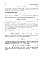
All the propagation characteristics can be modified by proper choice of the layer parameters.
For example, Fig. 2 shows dependences of the temperature coefficient of delay (TCD) on
quartz with single Al and Au layer on the second Euler angle and on the relative layer
thickness. Material constants for quartz are taken from (Shimizu and Yamamoto, 1980), for


a) b)
Fig. 2. Dependence of TCD (ppm/
o
C) on the 2
nd
Euler angle  and on the relative layer
thickness h/for Al (a) and Au (b). The first and third Euler angles are equal to zero.

Surface and Bulk Acoustic Waves in Multilayer Structures

83
Al and Au – from (Ballandras et. al., 1997). One can see in Fig. 2, that negative values of
TCD can be compensated by metallic layer. For example, orientation YX-quartz (0
o
,90
o
,0
o
)
becomes thermostable if h/ = 0.061 for Al layer and YX-quartz keeps the temperature
stability in range 0.027 ≤ h/ ≤ 0.032 for Au layer.
So, multilayer structures can be used both for protection against external undesired
influence and for improvement of the wave propagation characteristics, i.e. the SAW device
properties. All these possibilities can be evaluated by means of calculation technique,
described here.
3. Bulk acoustic waves in multilayer structures
Bulk acoustic waves are used in film bulk acoustic resonators. The simplest such resonator
contains at least three layers, namely an active piezoelectric layer, in which transformation
of the electric signal into the acoustic wave takes place, and two metallic (usually
aluminum) electrodes, connected to the source of the electric signal. The structure of such
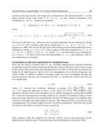
resonator (named membrane type resonator) is schematically shown in Fig. 3a.


a) b)
Fig. 3. Schematic view of the membrane type film bulk acoustic wave resonator (a) and of
the SMR resonator (b).
FBAR resonators are used in the ultra high frequency range (several GHz and higher),

therefore a thickness of the active layer is very small (microns and less). There are some
problems with mounting of such small structures on the solid massive and relatively thick
substrate. It is impossible to place membrane type FBAR on the substrate directly, because
in this case the useful signal will be deformed by multiple spurious oscillation modes due to
an acoustic interaction of the resonator and the substrate. To prevent this interaction more
complicated constructions are required. In particular, an air gap between the bottom
electrode and the substrate must be provided or cavity in substrate under a bottom
electrode must be etched. These variants require rather complex technological processes
application. Another possibility is mounting the multilayer Bragg reflector directly on the
substrate and then mounting of the resonator directly on this reflector. Such construction is
named a solid mounted resonator (SMR). The structure of such resonator schematically is
shown in Fig. 3b.
The Bragg reflector contains several (3 – 5) pairs of two materials with different acoustic
properties. The thickness of each layer in the reflector must be equal to a quarter of the
Electrode
Piezoelectric crystal
Electrode

Bragg reflector
Substrate

Waves in Fluids and Solids

84
wavelength in its material. Such construction provides attenuation of the wave and prevents
an acoustic interaction of the active zone of the resonator and the substrate.
Transversal sizes of the resonator are usually much larger than its total thickness, therefore
an analysis of all the main properties may be performed in the one-dimensional approach.
The most rigorous one-dimensional theory of such multilayer structures is presented in
(Nowotny and Benes, 1987). The following description is based on this theory, some

modified for expansion of its possibilities.
The wave equations, describing processes in the solid piezoelectric medium, are the same as
for surface acoustic waves – see (1) and (2). Assuming that all the values depend only on the
single spatial coordinate x
1
(mechanical displacements u
i
along all the coordinates x
i
take
place in this case nevertheless), we can write simpler form of these equations:

2
2
2
11 11
222
11
j
k
jk j
u
u
ce
xxt









j, k = 1, 2, 3 (39)

2
2
11 11
22
11
0
k
k
u
e
xx







(40)
Complex material constants (with real and imaginary parts) can be used for modeling of
electro-acoustic losses in the medium.
The solution for the electric potential

can be obtained from (40) in such form:

11
11 0
11
k
k
e
ux




 (41)
Here
0

and
1

are arbitrary unknown constants.
Substitution (41) into (39) gives:

2
2
_
11
22
1
j
k
jk

u
u
c
xt






(42)
Here
_
11
j
k
c are the stiffened elastic constants:

_
11 11
11
11
11
j
k
jk
jk
ee
cc


 (43)
We will seek the solution of these equations (j = 1, 2, 3) as a sinusoidal wave, propagating
along the x
1
axis with the velocity v:

1
1
()
1
(,)
x
it
ixt
v
kk k
uxt e e








 , (44)
where

= 1/v is a slowness.
Substitution of (44) into the equations (42) transforms them into the linear algebraic

equations system:

__
11jk
k
j
cc



, (45)

Surface and Bulk Acoustic Waves in Multilayer Structures

85
where

_
2
2
cv




(46)
In more detailed form the system (45) has the following view:

___ _
1111 1121 1131

12 3
____
1211 1221 1231
123
__ __
1311 1321
12 3
1331
() 0
() 0
()0
ccc c
cccc
cc cc


 



 


(47)
This is a system of linear equations for the three amplitudes







. This system can have a
nontrivial solution only if the determinant of its coefficients is equal to zero:

___ _
1111 1121 1131
____
1211 1221 1231
____
1311 1321 1331
0
ccc c
cccc
cccc




(48)
It gives the third power polynomial equation for
_
c , i.e. for

v
2
. Three roots of this equation
will represent the three eigenvalues
()
_
n

с (n = 1, 2, 3), giving three values of the bulk wave
velocity
v
(n)
or three values of the slowness

(n)
.
Three values
()n
k

(k = 1, 2, 3) correspond to each value
()
_
n
с . These values
()n
k

are
obtained by solving the system (47) for each value
()
_
n
с and represent the eigenvector.
System (47) is homogeneous, so its solution is determined up to an arbitrary factor.
Consequently, we can normalize each eigenvector by its modulus, and work further with
the normalized dimensionless vector. The three normalized eigenvectors are complete and
orthogonal:

() ( ) () ()
,
nm nn
nm kl
kk kl
n

 



(

kl
is the Kroneсker symbol) (49)
The general solution of the equations system (42) we will seek in such view:

11
(,) ()
it
kk
uxt uxe


 , (50)
where
u
k
(x

1
) is the linear combination of three bulk waves, obtained from equations (47) and
(48):

3
()
() () () ()
111
1
() [ cos( ) sin( )]
n
nn nn
k
k
n
ux A x B x
 



(51)

Waves in Fluids and Solids

86
Here A
(n)
and B
(n)
are six unknown coefficients of the linear combination. Together with

0

and
1

we have the eight unknown coefficients to be defined further.
We need the eight boundary conditions for obtaining the eight unknown coefficients. We
will use three normal components of the stress tensor, three components of the mechanical
displacement, the normal component of the electric displacement and the electric potential
for some concrete coordinate
x
1
, for example for x
1
= 0, as boundary values for unknown
coefficients determination.
The mechanical displacements and the electric potential are determined by expressions (51)
and (41) respectively, and for the stress tensor and for electric displacement the following
expressions are valid:
()
_
()
() () () () ()
111 11 1 1 111
11
[ sin( ) cos( )]
n
n
nn n n n
k

jj
k
j j
j
n
u
Tc e c A xB x e
xx


   


   


(52)

111 11 111
11
k
k
u
De
xx








(53)
Substituting
x
1
= 0 into (41) and (51) – (53), we get the following eight equations for
determination of
A
(n)
, B
(n)
,
0

, and
1

:

()
()
(0)
n
n
j
j
n
uA





()
_
()
() ()
1111
(0)
n
n
nn
jj
j
n
TcBe

 


(54)

1111
(0)D




11
0

11
(0) (0)
k
k
e
u




 (55)
Solving this system (taking into account the completeness and the orthogonality conditions
(49)), we can get all the unknown coefficients:
()
()
(0)
n
n
k
k
Au



11
()
()
11
()
_

11
()
1
(0) (0)
j
n
n
j
j
n
n
e
BTD
c











11
0
11
(0) (0)
k

k
e
u




11
11
1
(0)D



(56)
These coefficients (with using (41), (51) – (53)) give the possibility to obtain all the values
u
j
,
T
1j
, D
1
, and

for any coordinate x
1
, if these values are known for x
1
= 0 coordinate.

Let us consider in particular the single layer of thickness
l, infinite in lateral directions – see
Fig. 4.


Fig. 4. The single layer of thickness
l.
x
1
=
l

x
1
x
1
= 0

Surface and Bulk Acoustic Waves in Multilayer Structures

87
All the values u
j
, T
1j
, D
1
, and

for coordinate x

1
= l can be expressed as a linear combination
of these values for coordinate
x
1
= 0 in the following matrix form:
1
11 12 13 11 12 13 1
1
21 22 23 21 22 23 2
2
31 32 33 31 32 33 3
3
11
11 12 13 11 12 13 1
12
21 22
13
1
0
0
0
0
uu uu uu uT uT uT uD
uu uu uu uT uT uT uD
uu uu uu uT uT uT uD
Tu Tu Tu TT TT TT TD
Tu Tu
xl
MMMMMM M

u
MMMMMM M
u
MMMMMM M
u
T
MMMMMM M
T
MMM
T
D
















1
11
22

33
11 11
12 12
23 21 22 23 2
13 13
31 32 33 31 32 33 3
123123
11
0
0
0
1
00000001
Tu TT TT TT TD
Tu Tu Tu TT TT TT TD
uuuTTT D
x
uu
uu
uu
TT
TT
MMM M
TT
MMMMMM M
MMMMMM M
DD
 




 

 

 

 


















 


M

1
0x 













(57)

Here 8x8 matrix M is the transfer matrix of the single layer. This matrix allows to calculate
the values
u
j
, T
1j
, D
1
, and

on one surface of the layer via these values on another surface.
The elements of the transfer matrix are defined by wave equations solutions (i.e. by material
properties of the layer) by such a manner:

() ()
()
cos( )
nn
n
uu TT
ij ij
ij
n
M
Ml





() ()
() ()
1
sin( )
nn
nn
uT
ij
ij
n
M
l


 



(58)


() ()
() ()
sin( )
nn
nn
Tu
ij
ij
n
M
vl

 



()
() ()
11
1
sin( )
n
nn

uD T
i
ii
n
M
Mkl






(59)

()
()
()()
2
11
2sin
2
n
n
nn
TD u
i
ii
n
l
MM kv










() () ()
2
11
1
1sin()
nn n
D
n
l
M
kv l
l





 






(60)

Here

()
11
()
()
11
n
j
j
n
n
e
k
c



 (61)

In expressions (58) – (61) i, j = 1, 2, 3 (a number of the coordinate axis), n = 1, 2, 3 (a number
of the partial solution of the wave equations). The values k
(n)
, given by (61), are the
dimensionless scalar coupling coefficients (k
(n)

are nonzero only for piezoelectric medium).
One can see from the previous equations that the transfer matrix approaches to the unit
matrix if the layer thickness l
 0.
If a layer is nonpiezoelectric dielectric, all the elements of its transfer matrix, containing the
value k
(n)
, are zero, excepting
D
M

, and the transfer matrix of the nonpiezoelectric dielectric
layer has a simpler form:

Waves in Fluids and Solids

88

11 12 13 11 12 13
21 22 23 21 22 23
31 32 33 31 32 33
11 12 13 11 12 13
21 22 23 21 22 23
31 32 33 31 32 33
00
00
00
00
00
00

000000
uu uu uu uT uT uT
uu uu uu uT uT uT
uu uu uu uT uT uT
Tu Tu Tu TT TT TT
Tu Tu Tu TT TT TT
Tu Tu Tu TT TT TT
MMMMMM
MMMMMM
MMMMMM
MMMMMM
MMMMMM
MMMMMM

M
1
00000001
D
M

















(62)

For a metal layer in an electrostatic approximation the electric potential is always the same
on both its surfaces, therefore
D
M

= 0 for metal layer and the transfer matrix of the metal
layer has the simplest form:

11 12 13 11 12 13
21 22 23 21 22 23
31 32 33 31 32 33
11 12 13 11 12 13
21 22 23 21 22 23
31 32 33 31 32 33
00
00
00
00
00
00
00
uu uu uu uT uT uT
uu uu uu uT uT uT

uu uu uu uT uT uT
Tu Tu Tu TT TT TT
Em
Tu Tu Tu TT TT TT
Tu Tu Tu TT TT TT
MMMMMM
MMMMMM
MMMMMM
MMMMMM
MMMMMM
MMMMMM

MM
000010
00000001














(63)

The designation “M
Em
” will be explained further.
Now we can consider a multilayer system. Fig. 5 shows a multilayer structure with arbitrary
quantity N of arbitrary layers.


Fig. 5. Multilayer structure.
For multilayer structure the “output” values u
j
, T
1j
, D
1
and

of the first layer are the “input”
values for the second layer and so on. Therefore the transfer matrix of the multilayer
structure is a multiplication of the transfer matrices of each layer:
M = M
N

.
…
.
M
2
.
M

1
(64)
N
1
2
x
1
= 0
x
1
= l
1
+l
2
+…+l
N

x
1