Current Trends and Challenges in RFID Part 16 docx
Bạn đang xem bản rút gọn của tài liệu. Xem và tải ngay bản đầy đủ của tài liệu tại đây (1.76 MB, 30 trang )
Current Trends and Challenges in RFID
440
Zetter K. (2006). Hackers Clone E-Passports, 17.02.11, Available from:
/>1
22
Tag Movement Direction
Estimation Methods in an
RFID Gate System
Yoshinori Oikawa
NEC TOKIN Corporation
Japan
1. Introduction
An RFID system is desired to be introduced in large gate management systems because it
can read the ID of a large number of target objects simultaneously in the field of logistics
and retail business. Especially, UHF RFID has gathered significant interest since it has the
advantage of long distance reading and low cost of tags. Customers using an RFID gate
system require several convenient functions. One of them is to know the tag movement
direction for the purpose of recognition in warehousing or shipment for inventory
management. Moreover it can check for undesirable objects or prevent theft. For this
purpose, some sensors are established at the entrance and the exist side of the gate system in
an existing system. Therefore the direction of movement of tags is judged by the time
difference in the passing time at these sensors. For example, the future store of the Metro
group used this gate system for their stock management system of the backyard system [1].
However, in these systems it is necessary to use optional expensive equipment such as
several sensors.
In this chapter, an effective tag movement direction detection method is proposed in which
an original tag communication system is used as much as possible without using optional
equipment.
2. Estimation methods of the RF tag movement direction
It is basically necessary for the judgment of tag movement to obtain two or more time
information of an object. For obtaining that information, it is common to use two sensors on
both sides of the gate. This method corresponds to the Range-based method, which is a
location allocation system (LAS) method using a fixed anchor [2][3][4][5]. A conventional
RFID gate system using photoelectric sensors is shown in Fig.1. This gate can detect the
movement direction of an RF tag by judging the difference between the two passing times at
each sensor. For example, because the RF tag moves from the left side to the right side in the
case of Fig.1, sensor 1 detects it in advance of the detection at sensor 2. Here, a new method
of applying the Range-free method to RF tag direction detection is proposed.
Current Trends and Challenges in RFID
442
Reader
Antenna
Sensor2Sensor1
Tag
Fig. 1. Conventional RFID gate system
3. Proposed methods
3.1 Basic principle
Detection measures for measuring the time difference are considered for the RF tag and
reader antennas. A double antenna method using two antennas is proposed. The
configuration of this method is shown in Fig.2. The basic algorithm is that the tag movement
direction is estimated by measuring the time difference of two antennas. The merit of this
method is that the direction of each tag can be estimated independently. The conventional
sensor system can detect only for the bulk in the case of many tags. The proposed method
can estimate the movement direction for each tag even if some tags move in the opposite
direction toward the other tags simultaneously.
Target
tag
t=t
c
+ t
v m/s
t
c
x=v t
D
Reader
Antenna 2
Antenna 1
xa
d
Fig. 2. Double antenna method
3.2 Attributes for estimation
The types of information obtained from a tag is the read count, received power and
transmission delay. In this chapter, the former two types of information are studied because
they are simpler than the last one. Three methods are considered for judgment of the
detection time. They are (1) tag read time, (2) the time over the preset threshold, and (3) total
judgment that considers the detection pattern or weighted time. In the case of using the time
sequence pattern in the third method above, the processing function is very heavy because
of complication of its algorithm. That does not match the philosophy of Range-free.
Therefore, in this chapter, a weighted time center method for the third method is proposed.
Each method is shown in Table 1.
Tag Movement Direction Estimation Methods in an RFID Gate System
443
Attribute
Method
(a) Read count
(n)
(b) Recived power
(P
r
)
(1) Tag read
n1
-
(2) Threshold
1
nTh
r2
PTh
(3) Weighted
center
ii
i
i
i
(n t )
n
ri i
i
ri
i
(P t )
P
Table 1. Decision criteria of detection time
3.3 Basic model regarding received power
A basic model of an RFID system is shown in Fig. 3. The received power of a tag (chip) P
tr
and the received power of a reader P
r
are as follows using Friss’s formula [6].
tr t rt a tr
PPGLG (1)
rt rt atrm tta rr
trtrr trtt am
PPGLGLGLG
PGG GG 2LL
(2)
a
4
L20lo
g
d
(3)
Here, G
rt
and G
rr
is the transmission gain and received gain of the reader antenna, G
tt
and
G
tr
is the transmission gain and received gain of the tag antenna, L
m
is the internal loss of
the tag, L
a
is the propagation loss in the air, d is the read distance, λ is the wavelength.
Generally, the antenna of an RFID system can be used for both transmission and reception.
Therefore, let G
r
=G
rt
=G
rr
, G
t
=G
tt
=G
tr
, then eq. (1) and eq. (2) are
tr t r t a
PPGGL
(4)
rt r t a m
PP2GGL L (5)
Measurement results of P
r
in the case of P
t
=1W(30dBm), G
r
=6dBiC(circular polarization
antenna), G
t
=0dBil(linear polarization antenna) are shown in Fig.4. This shows that the
results are the same as the calculated values. Since the tag internal loss L
m
depends on
vendor or input level, the value of the actual used tag chip is applied.
Figure 4 shows that the distance (read range) between the reader and the tag can be
approximately estimated by measuring P
r
. In eq. (4) and (5), P
r
is a maximum when the tag
is just in front of the reader antenna. However, P
r
decreases as the tag moves into farther
from the center of the antenna because of its directional loss. Measurement results and
Current Trends and Challenges in RFID
444
calculated values of P
r
vs. the distance x between the center of the reader and tag are shown
in Fig.5. From Fig.5, the tag’s nearest point (x=0) to the reader can be estimated.
Reader
Modu-
lation
circuit
G
rt
G
tr
L
m
G
rr
G
tt
P
t
P
r
Read range: d
Propagation loss: L
a
Tag
Antenna Antenna
P
tr
P
tt
Fig. 3. RFID system model
0
50
100
150
200
250
300
350
400
00.20.40.60.811.21.4
M easured
Calculated
Read range d (m)
Received power P
r
(nW)
P
t
=30dBm
G
r
=6dBiC
G
t
=0dBil
Fig. 4. Read range vs Received power
3.4 Comparison of detection methods
3.4.1 Method 1
In Method 1, the starting time to read a tag is detected as shown in Table 1(1) even if read
only one time. In an actual RFID system, because tags are inventoried in advance of reading
the tag, the inventory time can also be used. This method is so simple. However, it is hard to
increase the decision accuracy since it sometimes happens to inverse the sequence of the
read time of the two antennas.
Tag Movement Direction Estimation Methods in an RFID Gate System
445
P
r
(nW)
0
10
20
30
40
50
60
70
80
-1.4-1-0.6-0.30.09 0.45 0.81 1.17
M easured
Calculated
-1 0 1-0.5 0.5
Distance from the antenna x (m)
Fig. 5. Measurement result (x vs P
r
)
3.4.2 Method 2
Incorrect judgment sometimes occurs due to a passing read for a reflected RF wave in the
case of Method 1.
Method 2 uses the threshold of detected values and judges the direction using the time
difference between each time when the detected value is over each threshold as shown in
Table 1(2). This method is able to increase the accuracy of detection. However, it is
sometimes hard to decide the threshold because the read count depends on the speed of
movement and the received power depends on the distance between the reader antenna and
the tag.
3.4.3 Method 3
Method 3 is proposed for improvement of the two methods, i.e. prevention of tentative read
error caused by the influence of reflection or null points. The principal of this method is to
estimate the time of the tag’s nearest position from the reader antenna. Wilson has proposed
the method for localization using the passive tag count percentage [7]. In this approach, tags
can be estimated the closest position by detecting the peak point. However, it is difficult to
adopt this method as RFID gate system because the variation of detected value reaches up to
several tens of meters and is equivalent to the distance between two antennas. Therefore the
algorithm we proposed is that each read time is weighted by the read count n or received
power P
r
, and the tag direction is estimated by the calculated difference between two
weighted centers of two antennas. Recently, RFID readers become to have high-performance
received power detection function [8]. Therefore, here, this method will be explained using
the received power as the tag attribute. Figure 6 shows the judgment procedure of the three
methods.
The detailed detection method is explained in Method 3. The received power is a function of
time actually because the tag goes through at a speed of v (m/s).
Eq.(5) is shown as eq.(6) from Fig.2 and Fig.5. Δt in Fig.2 is the time deference between the
passing time at the front of the reader antenna (t
c
) and the present time (t).
Current Trends and Challenges in RFID
446
0
10
20
30
40
50
60
0 2 4 6 8 10 12 14 16 18 20 22 24 26 28 30
0
10
20
30
40
50
60
0 2 4 6 8 1012141618202224262830
Th
ANT 1
ANT 2
Pr (nW)
Relative time t (s)
0 0.5 1.0 1.5 2.0 2.5 3.0
T1 T2
T1 T2
T1 T2
Method 3
Method 2
Method 1
Decision of
T1and T2
Read count
(n)>1
Pr>Th
Judge
T2-T1>0: ANT1ANT2
T2-T1<0: ANT1ANT2
(Pri ti)
ii
.
Pri
Fig. 6. Three methods in double antenna method
rt r t a m
P (t) P 2 G (t) G (t) L (t) L (6)
The estimation procedure is as follows.
When the certain time before the reader starts to read tags put t
0
, weighted center of read
time t
w1
(t
k
) and t
w2
(t
k
) from time t
0
to time t
k
of antenna 1 and antenna 2 are
k
r1 i i
i0
w1 k k
r1 i
i0
P(t)t
t(t)
P(t)
(7)
k
r2 i i
i0
w2 k k
r2 i
i0
P(t)t
t(t)
P(t)
(8)
where P
r1
(t) and P
r2
(t) are the received power of the two antennas at time t.
In the eq.(7) or (8), when t
w2
(t
k
)-t
w1
(t
k
)>0, it is judged that the tag moved from antenna 1 to
antenna 2, and when t
w2
(t
k
)-t
w1
(t
k
)<0, it is judged that the tag moved from antenna 2 to
antenna 1. The calculated results in the case of Fig.6 is shown in Fig.7.
When t
w1
and t
w2
in the case of stable values after the elapse of a certain period of time put
T1 and T2, respectively, the tag direction is finally judged by T2-T1 as shown in Fig.6 .
Tag Movement Direction Estimation Methods in an RFID Gate System
447
0
5
10
15
20
25
30
0 2 4 6 8 1012141618202224262830
t
w1
(t)
t
w2
(t)
Weighted center (t
w1
, t
w2
)
(s)
Relative time t (s)
0 0.5 1.0 1.5 2.0 2.5 3.0
0
0.5
1.0
1.5
2.0
2.5
3.0
(T2)
(T1)
t
w2
(t) - t
w1
(t)
Fig. 7. Shift with time of t
w1
and t
w2
in Method 3
Measurement results and the experimental environment using 10 dense tags are shown in
Fig.8 and Fig.9. Measurement conditions are shown below.
P
t
=30 dBm, G
r
=6 dBiC, G
t
=0 dBil, D=90 cm, xa=60 cm, v=1 m/s, height of antenna=1.3 m,
data rate=80 kbps, Reader: NEC TOKIN (Speedway)
Tags: UPM Raflatac ShortDipole
movement direction: from antenna 1 to antenna 2 (T2-T1>0)
Because the distance between two antennas that are the same type is 60 cm, T2-T1 becomes
0.6 seconds in theory. There are occasional erroneous decisions because of reflection or
interference in severe measurement environment, which causes undesirable reading in
method 1, and tags placed in the middle (e.g. tag #3, #4, #7 and #8 in Fig.8) are hard to read
in method 2.
On the other hand, method 3 is very stable because it is not misjudged, has low deviation
and a desirable average. Figure 10 shows the time transition of the difference t
w2
-t
w1
in
method 3. We can see this method can obtain a stable and correct result (expectant value in
the case of Fig.10 is 0.6s) even in the case of misjudgments caused by reflection and
interference in the measurement stage.
4. Measurement results in Method 3
4.1 Detection of the tag direction
The detail performance of Method 3 was measured. Figure 11 shows the tag read counts and
time difference T2-T1 in the case of two methods.
Though the deviation is wider in the case of a low read count, the judgment result is plus in
pattern 1, and minus in pattern 2. Therefore it has enough stability for use as an actual tag
direction decision tool. Pattern 3 shows the results in the illegal case assuming turning back
in the center of the antenna. In this case, the expectation value is 0. Figure 12 shows the
summary of means m and deviation σ of the measurement results of Fig.11.
By the way, an RFID system needs anti-collision technology that prevents no-read situations
caused by collision when many tags are read simultaneously. The sequence to read tags is
Current Trends and Challenges in RFID
448
-0.5
0.0
0.5
1.0
1.5
0123456 7891011
-0.5
0.0
0.5
1.0
1.5
01 2345 67891011
-0.50
0.00
0.50
1.00
1.50
01234567891011
T2-T1 (s)
1.5
1.0
0.5
0
-0.5
12345678910
12345678910
12345678910
(1) Method 1
Tag number
(2) Method 2
Tag number
(3) Method 3
Tag number
Calculated
Sample number: 10@tag
#1
#2
#3
#4
#5
#10
#9
#8
#7
#6
15cm
4cm
Tag array
m:0.54
:0.32
m:0.67
:0.31
m:0.63
:0.10
T2-T1 (s)
1.5
1.0
0.5
0
-0.5
T2-T1 (s)
1.5
1.0
0.5
0
-0.5
Fig. 8. Different time between two antennas
Tag Movement Direction Estimation Methods in an RFID Gate System
449
Antenna Reader
Tag array
#1
#2
#3
#4
#5
#10
#9
#8
#7
#6
15cm
4cm
Tag count per
each antenna
Display
Tag moving
direction
Tag identification
(EPC code)
Fig. 9. Photograph of experimental environment
-1.0
-0.5
0.0
0.5
1.0
0.0 0.3 0.5 0.8 1.1 1.4 1.6 1.9 2.2 2.5
1
2
3
4
5
6
7
8
9
1
0
Relative time t
(
s
)
t
w2
-t
w1
(s)
Calculated
Fig. 10. Relative time vs (t
w2
-t
w1
) in method 3
Current Trends and Challenges in RFID
450
Moving pattern:
ANT1 ANT2
(3) 80kbps
Tag number
(4) 640kbps
Tag number
T2-T1 (s)
Sample number: 10@tag
12345678910 12345678910
(1) 80kbps
Tag number
(2) 640kbps
Tag number
12345678910 12345678910
0
10
20
30
40
50
60
70
80
Count number
11
22
33
11
22
33
11
22
+
-1.5
-1.0
-0.5
0
0.5
1.0
1.5
Fig. 11. Relative time vs (t
w2
-t
w1
) in method 3
random because a typical anti-collision system is used for using the probabilistic approach
[9]. A variation of tag read sequence directly becomes a validation of detection time
difference. Therefore, when a weighted center is normally-distributed, the time difference
T2-T1 is also independent and identically distributed because of its reproducing property.
From Fig.12, it is assumed that the criteria of detection precisely is 3σ or less, and the tag
direction can be judged correctly from the data of pattern 1 and pattern 2. However, a data
rate up to round 640kbps is necessary when the difference from abnormal action such as
turning needs to be detected (pattern 3 in Fig.12).
Tag Movement Direction Estimation Methods in an RFID Gate System
451
80kbps 640kbps
Data rate
T2-T1 (s)
0.9
0.6
0
-0.3
-0.6
0.3
-0.9
Moving
pattern
: Average (m)
: m-(T2-T1) < 3
11 22 33 11 22 33
Fig. 12. Measurement results of (T2-T1)
4.2 Estimation of the tag moving speed
The detail performance of Method Moreover, the speed of movement can be also estimated
by measuring the time difference T2-T1 because the distance between two antennas is fixed.
Figure 13 shows the measurement results of the movement speed.
Variation of measurement results in the case of v=2m/s is larger than in other cases because
the precise speed is inversely proportional to the speed of movement of the measurer.
Figure 13 shows that this method can estimate not only the tag direction but also the speed
of movement. It is very useful to set the threshold Th of movement speed as the decision
criteria in order to increase the accuracy. For example, when the threshold Th1 and Th2 are
set to -3.5 and 3.5 respectively, it is possible to eliminate abnormal movement such as
turning in Fig.13.
-5
-4
-3
-2
-1
0
1
2
3
4
5
-4
-3
-2
-1
0
1
2
3
>5
Moving speed (m/s)
(1) 0.5m/s (2) 1m/s (3) 2m/s (4) U turn
m:0.59
:0.08
m:0.93
:0.08
m:2.09
:0.40
-
m:-0.51
:0.08
m:-0.94
:0.13
m:-2.02
:0.39
-
<-5
4
Fig. 13. Measurement results of moving speed
Current Trends and Challenges in RFID
452
4.3 Effect of the orientation of the tag
Generally, a tag are used a liner polarized dipole antenna in consideration of read range and
cost. In this case, the read performance in reader depends on the orientation of the tag. The
tag movement detection results of the time difference T2-T1 in three cases is shown in
Fig.14.
-0.50
0.00
0.50
1.00
1.50
01234567891011
-0.50
0.00
0.50
1.00
1.50
01234567891011
-0.50
0.00
0.50
1.00
1.50
01234567891011
T2-T1 (s)
1.5
1.0
0.5
0
-0.5
12345678910
12345678910
12345678910
(1) Angle of 0 degrees
Tag number
(2) Angle of 45 degrees
Tag number
(3) Angle of 90 degrees
Tag number
Calculated
Sample number: 10@tag
(1)
T2-T1 (s)
1.5
1.0
0.5
0
-0.5
T2-T1 (s)
1.5
1.0
0.5
0
-0.5
ANT
(2) (3)
Angle of tags
Fig. 14. Different time between two antennas
Tag Movement Direction Estimation Methods in an RFID Gate System
453
T2-T1 of the tags that have 90 degrees angle against the reader antenna ((3) in Fig.14) varies
widely because they are hard to be read. The percentage of read in this case was 79% and
the accuracy among tags to be read was 95%. However, when tags set 45 degrees angle, the
movement direction of tags can be detected with as high accuracy as a parallel case ((1) in
Fig.14). In other words, it is useful to tilt two antennas of the reader in place of tags.
4.4 Effect of the intersection of the tags
In actual cases, it may happen that two tag groups pass through in the opposite direction
individually and simultaneously. The measurement results in that case are shown in Fig.15.
Moving direction: Both way
(cross in the center)
ANT1 ANT2
(1) Data rate: 80kbps
Tag number
(2) Data rate: 640kbps
Tag number
T2-T1 (s)
12345678910
0
10
20
30
40
50
60
70
80
Count number
-1.5
-1.0
-0.5
0
0.5
1.0
1.5
Reader
11121314151617181920
#11
#12
#13
#14
#15
#20
#19
#18
#17
#16
Tag array
12345678910
11121314151617181920
12345678910
11121314151617181920
12345678910
11121314151617181920
Simultaneously
90cm
150cm
#1
#2
#3
#4
#5
#10
#9
#8
#7
#6
11
2
2
11
2
2
1122 1122
Sample number: 10@tag
Fig. 15. Measurement results in simultaneous cross moving
Current Trends and Challenges in RFID
454
One tag group (#1-#10) passed through from antenna 1 to antenna 2, and the other group
(#11-#20) passed through in the opposite direction behind the former group. Tag group (#1-
#10) has the same characteristics as in Fig.11. However, tag group (#11-#20) is strewn
widely because the radio wave is blocked by the other tag group in passing in front of the
reader antenna. In the case of 80kbps data rate, 14% of this tag group could not be read and
around 5% among all the read tags made an error (that is, the accuracy was about 95%).
However, when the data rate is 640kbps, both of the read rate and the accuracy are 100%.
Therefore, this method is useful because the tag moving direction can be detected correctly
by increasing the data rate even if the most severe case like intersection in front of the
antenna.
5. Conclusion
In this chapter, a method for precisely estimating the tag movement direction in an RFID
gate system was proposed. This method uses the time difference between two antennas of
the reader. This method has the advantage of being able to judge tag direction individually
even when there are some tags moving to the reverse direction. Especially, when it uses the
proposed algorithm of the weighted center of passing time, the precision of the estimation
can be increased. Finally, the feasibility of the method was proved by measurement results.
6. References
[1] “Metro Future store”
[2] H. Ochi, S. Tagashira and S. Fuita, “A localization system for wireless sensor networks,”
IPSJ SIG Tech. Rep., ARC-160, pp.17 22, Dec.2004
[3] T. He, C. Huang, B. John, A. Stankovic and T. Abdelzaher, “Range-free localization
schemes for large scale sensor networks.” Mobicom, September 2003, pp.81 93
[4] J. Hightower, G. Borriello and R. Want, “SpotON: an indoor 3D location sensing
technology based on RF signal strength” UW CSE Tech. Report #2000-02-02,
February 2000
[5] L. Ni, Y. Liu, Y. Lau and A. Patil, “LANDMARC: indoor location sensing using active
RFID” Wireless Networks 10, pp.701 710, Kluwer Academic Publishers,
Netherlands, 2004
[6] T. Yoshikawa, “Radio engineering B,” Tokyo Denki University
[7] P. Wilson, D. Prashanth and H. Aghajan, “Utilizing RFID signaling scheme for
localization of stationary objects and speed estimation of mobile objects”
International conference on RFID, pp.94 99, March 2007
[8] Y. Oikawa, “UHF IC tag and reader/writer products” NEC Tech. Journal, vol.2, No.4,
pp.76 80, December 2007
[9] Y. Kawakita, J. Mitsugi, O. Nakamura and J. Murai, “Acceleration of UHF-band RFID
inventory leveraging capture effect.” IEICE, vol.J91-B, No.10, pp.1279 1286,
October, 2008
23
Third Generation Active RFID from the
Locating Applications Perspective
Eugen Coca and Valentin Popa
Faculty of Electrical Engineering and Computer Science
Stefan cel Mare University of Suceava
Romania
1. Introduction
Location systems, both for indoor and outdoor use, are rapidly developing due to the
practical need of knowing the position of objects and persons (Harrop, 2008). If for the
outdoor world, the GPS system and its variants (DGPS, etc.) is the best possible solution, for
indoor use, things are not yet completely solved. Indoor GPS is developing, but in parallel,
other projects are running. The vast majority of papers dealing with the subject (Bess, 2009;
Chang et al., 2011; Goncalo, 2009; Kathiravan et al., 2009; Khan & Antiwal, 2009; Jeon et al.,
2010) present systems based on RF signal measurements. Multiple ways of solving the
problem are technically imaginable, starting with those using the signals emitted by the
nodes of a common WLAN / Wi−Fi wireless network (Bal et al., 2009; Clulow et al., 2006;
Kaemarungsi & Krishnamurthy, 2004; Kushki et al., 2006; Kwon & Song, 2008; Tsui et al.,
2010; Yousef & Agrawala, 2005), continuing with RFID systems, WSN networks and
finishing with proprietary solutions derived from one of the above, where specialized nodes
with one or more coordinators are deployed over the desired locating area (Bahl &
Padmanabhan, 2000; Baunach et al. 2007; Chang et al. 2011; Coca et al. 2008; Dai & Su, 2008;
Koyuncu & Yang, 2010).
RFID tags are the main factor of progress in identification application development. There
are more than 40 year from the first generation (Finkenzeller, 2003), equipped with passive
components where the energy is captured from the radio−frequency field generated by the
reader, to the third generation where the energy supplied by a battery is used to power a
microcontroller and one or several on−board sensors. In terms of price, in 2011 the passive
tags may be found at prices as low as 0.05 USD each, whereas the active RFID tags equipped
with complex sensors and low−power microcontrollers may cost as much as 100 USD a
piece (Harrop, 2008).
From the point of view of RFID tag structure, the changes are obviously influenced by the
progress in semiconductors technology. The software for the reader and applications
evolved also on the same trend. For the Generation 1 UHF tags, manufacturers provide
hardware with their own protocols. Therefore, tags from one specific manufacturer would
only work with the RFID reader from the same manufacturer. From the point of view of
users, this represents a major limitation and for large-scale implementations, single supplier
solutions are not acceptable. Generation 2, the second-generation RFID UHF tags, developed
in order to establish a standard for RFID tags, used by the big retailer inventory applications
Current Trends and Challenges in RFID
456
and operating in the ultrahigh frequency (UHF) band (860−960 MHz), offer long range
operating distances (at least 8 to 10 meters). A comparison between the differences between
Gen 1 and Gen 2 protocols may be found in Table 1 (EPC, 2005).
Four UHF RFID standards exist: Class 0 and Class 1 − from EPCglobal, and 18000−6 Type A
and Type B from ISO. ISO's 2006 approval of Gen 2 as an 18000−6C extension opened the
way to a single UHF global protocol. Such a protocol will create an open market as well as
an open standard, which will force the prices to go down. Even the great efforts made in the
direction of unifying the standards, a large RFID market with a strong supply chain and
industrial backbone − China, has not accepted either the ISO or EPCglobal standard.
Instead, China hopes to develop own standards compatible with Gen−2 tags, their readers
being able to communicate with the standard tags (Bijl & Dil., 2010; Roberti, 2005; Razaq et
al. 2005).
Gen 2 frequency range is from 860 to 960 MHz and it covers all international frequency
spectrums. Tags that comply with EPCglobal's Gen 2 standard operate between these ranges
without performance degradation. Gen 1 didn't do well in Europe due to European radio
frequency spectrum allocation didn't leave enough open bandwidth for US radio
frequencies, but Gen 2 offers Europe's required frequency range of 865 to 868 MHz, while
fulfilling US frequency sub band of 902 to 928 MHz. The ISO 18000−6C extension makes
Gen 2 a real flexible international standard (Jong & Bijl, 2010; Roberti, 2005; Razaq et al.
2005).
Description Gen 1 Gen 2
Acceptance level Not a global standard
Global standard after an
amendment in
ISO−UHF 18000−6 standard
Arbitration
Deterministic binary tree for
Class 0 and deterministic
slotted for Class 1
Probabilistic slotted
Anticollision/tag-sorting
algorithm
Binary tree algorithm with
persistent state/wake
states
Q algorithm, which is a
variant of the slotted
aloha protocol
Air interface Pulse width modulation
(PWM) for Class 0 and
Class 1
Pulse interval encoding
(PIE−ASK), Miller, FM0
Data rate 40/80 Kbits for Class 0 and
70/140 bits for Class 1
40 to 640 Kbits
Distance Less than 10 meters Less than 10 meters
Frequency range 850–930 MHz 860 to 960 MHz
Security password
8 and 24−bit passwords,
respectively, for Class 1
and Class 0
32 bits
Data write verification No Yes
Write speed (for 96−bit
electronic product code)
Three tags per second Minimum five tags per
second
Table 1. Main differences between the Gen 1 and Gen 2 protocols
Third Generation Active RFID from the Locating Applications Perspective
457
The working frequency is a key design issue in RFID locating systems. The ability for signals
to propagate within crowded environments is dependent on the signal wavelength. Within
warehouses, truck yards, office buildings, and other industrial or commercial facilities, the
ability for an RFID system to operate in and around obstructions is critical (Han et al., 2008;
Hsu et al., 2009; Jeon et al., 2010; Kiang et al., 2009). These obstructions are often made of
metal, such as vehicles and metal racks, requiring signals to propagate around rather than
through them. Signals propagate around obstructions by means of diffraction, and the level
of diffraction is dependent on the size of the object over the signal wavelength ratio.
Diffraction occurs when the wavelength approaches the size of the object. For example, at
433 MHz the wavelength is approximately a meter, enabling signals to diffract around
vehicles, containers, and other large obstructions.
Regarding the frequencies used by active tags systems regulations, a summary is presented
in Table 2:
Band
303
MHz
315 MHz
418 MHz
433 MHz
868 MHz
915 MHz
2400
MHz
Working
frequency
band
302−305
MHz
314.7−315
MHz
42
dBuA/m
@10m
418.95−
418.975
MHz
10 mW
ERP
433.050−
434.790
MHz
10mW
ERP
10%
868−868.6
MHz
25mW
ERP
1%
902−928
MHz
2400−248
3.5
MHz
USA x x x x x x
Canada x x x x x x
UK x x x
France x x x
Germany x x x
Netherlands x x x
Singapore x x x x
Taiwan x x x x x x
China x x x
Australia x x x
Table 2. Summary of global frequency regulations for the most common Active RFID bands
At 2.4 GHz, the wavelength is approximately 10 centimeters and diffraction is very limited
with these obstructions, creating blind spots and areas of limited or even no coverage.
Frequencies above 2 GHz present significant challenges for operation in crowded
environments and are therefore not recommended for most RFID applications.
One may notice only 433 MHz and 2400 MHz working frequencies bands systems are
allowed in almost all countries. Even both frequency bands overlap with the ISM bands,
these are the most accepted in the RFID world. Despite in the 2400 MHz band there are
many wireless systems (Wi-Fi, Bluetooth, ZigBee, etc.) making the frequency spectrum very
crowded, producers continue to develop new systems and communication protocols
working in this free band, design simplicity, small dimensions and low power consumption
being solid arguments for continuing the researches.
Current Trends and Challenges in RFID
458
2. RFID systems in localization applications
Real Time Locating Systems (RTLS) help users to locate and track objects in real-time. This
could be done in many ways, along the time different technologies being developed around
the idea. The RTLS term was introduced in 1988 to describe a technology that provided the
Automatic Identification capabilities of active RFID, but added the ability to see the physical
location of the tagged object.
From the locating perspective, the RFID has a long history. Conventional active RFID tags
are the first used for real time locating applications. Starting with Gen 2 tags, the EPCglobal
Class−1 Generation−2 UHF RFID Protocol for Communications standardized the active tags
working in 860 − 960 MHz frequency band (EPC, 2005). The included battery helps them to
initiate a signal, giving longer range compared to passive tags. This type of tags are mostly
known for the end users as locking the cars as over two billion dollars were spent on car
clicker systems to date (Harrop, 2008). Millions of other tags were also deployed in postal
services monitoring applications, and supplies or assets management. Localization systems
were developed for this type of active tags, an example being the RFID radar (RFID−Radar,
2005). RFID radar is a mixed localization system, based on both ToA − Time of Arrival and
AoA − Angle of Arrival methods (Coca & Popa, 2007). It uses a system based on one
emitting and two receiving antennas. The working principle, based on a tag-talks-first
protocol (Coca et al., 2008), is as follows: when a transponder enters the area covered by the
emitting antenna, it will send its ID and memory content. Two dedicated antennas receive
the signal transmitted by the transponder. Based on the time difference between the two
received signals and the range information, it computes the angle and the distance. The
system uses a central frequency of 870.00 MHz with a bandwidth of 10 kHz. The
performances in term of localization precision are modest, even the location information is
available for tags placed up to 40−45 meters in front of the antennas (Popa et al., 2010).
The second generation of active RFID tags is present in the true Real Time Locating Systems
(RTLS) used today for continuous monitoring applications. The active tag includes a battery
used also to supply the on-board sensors and a low power microprocessor, improving the
capability to store the measured data over a significant period. When using many readers,
distances over several hundred meters are usually obtainable. Even these systems were
initially designed for assets tracking, localization applications were position and speed
information were added as a plus. In terms of location precision, it is strongly influenced by
the reflections on obstacles and moving objects positioned between the reader and the tags.
The third generation of active RFID tags overlaps with the well-known Wireless Sensor
Networks (WSN) or Ubiquitous Sensor Networks (USN) (Bess, 2009; Harrop, 2008). The
most important characteristic of the tags is they communicate one with each other and in the
same time with the central node. A central node, named also the coordinator or the gateway,
pays the role of the RFID reader from a classic system. Even the maximum distance between
the two nodes is limited to 10 to 30 meters (mainly due to maximum power emission
regulatory restrictions but also due to attenuation, reflections and interference with other
systems), the networks could be easily extended over hundreds of meters or even more,
based on the inter−nodes communications capabilities.
3. Third generation RFID system in localization applications
Wi-Fi technologies, developed for delivering wireless communications between mobile
terminals, are also used in locating applications by processing the identification data from
Third Generation Active RFID from the Locating Applications Perspective
459
multiple Access Points (AP) and the Received Signal Strength Indication (RSSI)
information.
The signal strengths of received signals from at least three access points are used to
determine the location of the object being tracked. To increase accuracy, more sophisticated
methods use RF fingerprint maps that are based on calibrations of the strength of Wi-Fi
signals at various points in a predefined area. Applications using Wi-Fi combined with Time
Difference of Arrival (TDOA) techniques were also developed.
In an RSSI system, the distance between a tag and a reader is computer by converting the
value of the signal strength at the reader into a distance measurement, based on the known
signal output power at the tag and on a particular path loss model.
Wi-Fi location technique has some advantages over other systems:
- It uses the existing infrastructure;
- Position information is available both at the coordinator and at each node, information
that could be shared with neighbor nodes.
Some major disadvantages of these systems include:
- Signal power measurements are affected by fixed and mobile objects, thus generating
random measuring errors, even a power map was created for the specified measuring
area;
- Network traffic congestions affect the system availability and the results;
- Power consumption is higher compared to RFID or WSN solutions.
To be effective, RSSI requires a dense deployment of Access Points, which adds
considerably to the systems cost. The key problem related to RSSI based systems is that an
adequate path loss model must be found for both non-line-of-sight and non-stationary
environments. In practice, the estimated distances are not quite precise. RSSI locating
systems may also be disqualified from security applications as an attacker can easily alter
the strength of received signals by amplifying or attenuating it, or by other methods
distorting the signal strength received from one more Access Points used as fixed
references.
The disadvantages above made the Wi-Fi locating system not to develop as rapid as other
technologies did, and positioning system solutions based on it are not widely spread in the
real world.
RFID locating implementations were investigated and test setups are already used in real
world applications both for indoor or outdoor locating services, even this technology was
created as a bare code replacement. RFID systems were initially developed with the need of
data storage in mind, and other aspects were not taken into consideration. Many efforts
were done in order to modify RFID systems and make them suitable for indoor locating
applications. A proprietary system derived from a RFID system (RFID Radar, 2005) is a
good example for outdoor and indoor location, as only a small quantity of information is
transmitted, the processing power being used for position estimation. One of the major
disadvantages of such systems is the user is unable to modify the application or to write his
own code due to copyright restriction. Communication protocol details are not always
completely disclosed, so creating new system configurations could be a difficult task. In
addition, the high power level used by the system makes it unsuitable for indoor location
application or for populated areas (Coca et al., 2008).
The third generation RFID systems have the characteristics of a network of wireless sensors,
the nodes being the tags. There are even no notable differences between the active RFID tags
and WSN nodes, as both are powered from external energy sources, contain sensors and
Current Trends and Challenges in RFID
460
small data processing capabilities. This is the reason the research was focused on the WSN
networks for using them in applications where standard active RFID systems were unable to
deliver the required performance levels.
Wireless Sensors Networks contains nodes with one or more sensors connected with a RF
transceiver. When multiple WNS nodes are deployed over an area, signals transmitted by
them could easily used for location purposes. The performances in the cited literature (Buta
et al., 2010; Halgamuge et al., 2009; Kim & Yang, 2008; Jeong & Nof, 2008; Kuang et al., 2008;
Lanzisera et al. 2004; Mao et al., 2007; Miorandi et al., 2007, Ota & Wright, 2006) are low
enough to justify future investigations. For stationary environments, especially for indoor
situations, location of objects is a relatively easy task. When moving objects have to be
located and eventually traced, the WSN is a challenging solution. The typical structure of a
third generation RFID locating network is shown is Figure 1. The message transmitted from
one node to the gateway contains the node IDentification data along with the physical
coordinates.
Fig. 1. Typical third generation RFID locating network overview
The position information may be obtained from on-board sensors (like GPSs,
accelerometers, etc.) or may be computed from the information received from nearby nodes
(RSSI is the most common information computed in order to obtain position information).
The key of this architecture is the communication protocol that allows the information to be
transmitted from one node to the gateway through any available path. This way in the event
a node is not available, the information is routed through the healthy nodes.
4. Experimental results
4.1 Test system characteristics
For performance evaluation, we used a Wireless Sensor Network development system from
Green Peak Technologies (GreenPeak, 2010). The system consists of a coordinator node
Third Generation Active RFID from the Locating Applications Perspective
461
(known as Gateway) and nine nodes, operating in the ISM band (2.4 GHz), with 16 channels
and 250 kbps data rate and is certified to meet EN 300 440 (Europe), FCC CFR47 Part 15 (US)
and ARIB STD−T66 (Japan) standards. The node architecture is presented in Figure 2:
Fig. 2. WSN node architecture
The node is built around an Atmel AVR 1281 microcontroller and powered by 3 AAA
batteries (Figure 3). On the board, there are temperature and humidity sensors, analog and
digital inputs. In complex applications, the node may be upgraded to support a more
powerful processor and multiple inputs.
In terms of operating distance, the typical values declared by the producer vary from 40−100
meters indoor, to 160−400 meters outdoor and up to 1000 meters outdoor in light−of−sight
view. In the presence of blocking objects, shorter ranges are expected. The gateway is
equipped with a RISC processing unit and a RF module, very similar with the one on the
node.
Fig. 3. WSN sensor node with integrated temperature sensor (Power provided by 3 AAA
bateries placed underneath)
Current Trends and Challenges in RFID
462
The WSN Gateway has a wireless communication module connected to its interface board
(Figure 4), allowing TCP/IP, USB or RS232 serial communication with the external world
(the processing software installed on a standard PC). The main characteristics of the
communication stack are:
- Mesh network: messages travel from source node to destination node through
intermediate nodes thereby multiplying range as a function of number of hops. The
multi-hop feature does not require any application intervention.
- Self-forming: mesh network forms automatically, without any application intervention
- Self healing: when individual links fail the mesh network reestablishes a reliable route
autonomously
- Security: data transfer through message encryption (AES 128 bit)
- Support for mobile nodes: Nodes can physically move through the network without
requiring network re-association
- Support for ultra low power end devices: Reduced functionality devices can operate for
years without replacing batteries
- Support for network visualization: network topology can be visualized using the
optional JadeMonitor PC software component
- Robust against interference: able to operate in the presence of other wireless devices
such as Wi-Fi, Bluetooth and others
- Scalability: the network can scale up to 100s of nodes without reconfiguration
Fig. 4. Gateway/Coordinator node built around a RISC microcontroller
From the communication protocol side, we have to choose between 2 types of network
stacks, namely PeakNetZ and PeakNet LPR. The API to both stacks is almost identical. The
different properties are given in Figure 5.
In applications where the nodes have access to mains power instead of batteries and some
devices operate on batteries, the PeakNet™ Z is the best solution. The network consists of
Full Functionality Devices (FFD), Reduced Functionality Devices (RFD) and one or more
Third Generation Active RFID from the Locating Applications Perspective
463
Network Coordinators. All FFDs automatically become part of the wireless mesh networks
and take active part of routing messages.
Sensors may be connected to these nodes. The RFDs nodes interface to sensors and actuators
and connect wirelessly to a nearby FFD. As they are set in a sleeping−state most of the time,
they consume very little power. The RFD will not actively route messages for other devices.
The Network is self−healing and self−forming and is managed by the coordinator
node(GreenPeak, 2010).
When all nodes are battery−powered, PeakNet™ Low Power™ (LPR) is the most
convenient solution. PeakNet LPR does not require always−on, mains−powered devices. All
devices are in low−power state and still form a mesh and route messages through the
network. The low−power routing meshing capability is obtained by occasionally waking up
the low power nodes along a synchronized scheme.
Fig. 5. The 2 types of network stacks PEAKNET
TM
Z (left) and PEAKNET
TM
LPR (right)
(GreenPeak, 2010)
Hence, devices can pass messages through the network and in the same time conserve the
battery power. Devices can be woken up according to a pre−defined schedule or when an
external event occurs, or on a combination of both.
When powered up, the nodes automatically associate to the coordinator node. This
coordinator also functions as a serial gateway: it allows the user to access the remote nodes
in the network from a PC connected to the coordinator module.
All the software necessary for the network to work is embedded in the coordinator node.
This means that the network can run stand−alone, without attaching a PC to the
gateway/coordinator module.
The development software offered by the producer has an interface showing each node
relative to other nodes positions. A map of the installations location permits to calibrate the
distances and to display the real positions of all nodes having the coordinator node as a
reference. For each node, the software displays the information read from the sensors and