Recent Advances in Vibrations Analysis Part 2 pot
Bạn đang xem bản rút gọn của tài liệu. Xem và tải ngay bản đầy đủ của tài liệu tại đây (402.95 KB, 20 trang )
Exact Transfer Function Analysis of Distributed
Parameter Systems by Wave Propagation Techniques
9
1
() () ()
ii ii i i i i
w
f
C
f
C
(2.30)
However, due to Eq. (2.19)
1
()[() () ]
ii ii i i ir i
w
ff
RC
(2.31)
Now by applying the global wave transmission coefficient defined in Eq. (2.25) to
i
C
in the
above equation, the displacement at any point in span
i of the string can be expressed in
terms of the wave amplitude in span
i1 as
1
1
()[() () ]
ii ii i i irii
w
ff
RTC
(2.32)
Assume a disturbance arise in span 1; i.e., a wave originates and starts traveling from the
leftmost boundary of the string. Then, by successively applying the global transmission
coefficient of each discontinuity on the way up to the first span, the mode shape of span
i
can be found in terms of wave amplitude
1
C
; i.e.,
1
1
1
()[() () ]
ii ii i i ir j
ji
w
ff
RTC
1
C
0
ii
l
(2.33)
0246810
-2
-1
0
1
2
3
2
F(
)
1
Fig. 3. Plot of the characteristic equation. The solid and dashed curves represent the real and
imaginary parts, respectively.
For example, consider a fixed-fixed undamped string with three supports specified by
2
=5+0.1s
2
,
3
=7+0.1s
2
, and
4
=4+0.1s
2
according to Eq. (2.13). l
1
0.25, l
2
0.3, l
3
0.25, and
l
4
0.2 are assumed. Once the global wave reflection coefficient at each discontinuity has
been determined, one can apply Eq. (2.29) to find the natural frequencies. Shown in Fig. 3 is
the plot of the characteristic equation, where the first three natural frequencies are indicated.
The mode shapes can be found from Eq. (2.33) in a systematic way once the global wave
transmission coefficient at each discontinuity has been determined. Figure 4 shows the
mode shapes for the first three modes.
Recent Advances in Vibrations Analysis
10
0.0 0.2 0.4 0.6 0.8 1.0
-3
-2
-1
0
1
2
3
w
x
Fig. 4. First three mode shapes obtained from Eq. (2.33). The solid, dashed, and dotted
curves represent the 1
st
, 2
nd
, and 3
rd
modes, respectively.
2.4 Transfer function analysis
Consider a multi-span string subjected to an external point load ()
p
s , normalized against
tension
T, applied at xx
0
as shown in Fig. 5. Since the waves injected by the load travel in
both direction from the point of loading, a set of local coordinates {
,
*
} is introduced such
that the wave traveling toward each boundary of the string is considered positive as
indicated in Fig. 5. Let
1
C
and
1
D
denote the injected waves that travel in the region x<x
0
and
xx
0
within span 1, respectively. The transverse displacement of span 1 of the string can
be expressed as
Fig. 5. Wave motion in a multi-span string due to a point load.
1
110 11 1 1 1 1
( , ;) ( ;) ( ;)wxs
f
sC
f
sC
11
0 l
(2.34)
Defining
v as the wave injected by the applied load, the difference in amplitudes between
the incoming and outgoing waves at the loading point is
11
CDv
11
DC v
(2.35)
2
D
1
D
*
2l
R
*
1r
R
1
D
*
nl
R
1
C
1r
R
2l
R
1
C
n
1
*
m
*
2
r
R
nl
R
2
D
1
2
C
2
C
2 1 2
*
0
xx
()
p
s
Exact Transfer Function Analysis of Distributed
Parameter Systems by Wave Propagation Techniques
11
where v can be determined from the geometric and kinetic continuity conditions at
=0 as
1
()
2
vps
(2.36)
Applying the global wave reflection coefficient on each side of the loading point gives
111r
CRC
*
111r
DRD
(2.37)
where the asterisk (
*
) signifies that the global wave reflection coefficient is defined in the
region xx
0
to distinguish it from the one defined in the region x<x
0
. Combining Eqs. (2.35)
and (37), one can determine the ampltitude of the wave that rises at the loading point in
each direction
11
CTv
**
1111
(1 )(1 )
rr r
TRRR (2.38.1)
*
11
DTv
**
1111
(1 )(1 )
rr r
TRRR (2.38.2)
Note that
1
T and
*
1
T and can be considered as the global wave transmission coefficients that
characterize the transmissibility of the wave injected by the external force in the region x<x
0
and xx
0
, respectively. It is evident that and
1
T and
*
1
T are different unless the string
system is symmetric about the loading point. Applying the results in Eqs. (2.37) and (2.38) to
Eq. (2.34), the wave motion in either side of x=x
0
can be found; i.e., in the region x<x
0
1
110 11 1 1 1 1
(,;)[(;) (;) ]
r
wxsfsf sRTv
11
0 l
(2.39)
Now, in the same manner as for the mode shape analysis, since
1iii
CTC
and
11
CTv
,
the wave motion in span i on either side of the loading point can be found. For the region
x<x
0
1
1
0
( , ;) [ ( ;) ( ;) ]
ii ii i i ir k
ki
wxsfsf sR Tv
0
ii
l
(2.40)
Note that the ratio
00
( , ;) ( , ;) ()
ii ii
Gxswxsps
(2.41)
is the transfer function governing the forced response of any point in span i due to the point
loading at xx
0
. The Laplace inversion of G
i
(
i
, x
0
; s) is the Green’s function of the problem.
Thefore, denoting L
1
as the inverse Laplace transform operator, the forced response at any
point within any subspan of the multi-span string can be determined from the following
convolution integral; e.g., for span i in the region x<x
0
00
0
(, ;) (, ; )()
ii ii
wx Gx
p
d
( 1,2, ,im
) (2.42.1)
1
11
01
1
(, ;) [ [(;) (;) ] ]
2
ii ii i i ir
ki
Gx L
f
s
f
sR T
0
ii
l
(2.42.2)
Recent Advances in Vibrations Analysis
12
The exact Laplace inversion of G
i
(
i
, x
0
; s) in close form is not feasible in general, in
particular for multi-span string systems. One may have to resort to the numerical inversion
of Laplace transforms. It is found that the algorithm known as the fixed Talbot method
(Abate & Valko, 2004), which is based on the contour of the Bromwich inversion integral,
appears to perform the numerical Laplace inversion in Eq. (2.42) with a satisfactory accuracy
and reasonable computation time. In this method, the accuracy of the results depends only
on the number of precision decimal digits (denoted with M in the algorithm) carried out
during the inversion. It is found that for well-damped second- and higher order distributed
parameter systems, M32 and for lightly damped or undamped systems, M64 gives
acceptable results. To demonstrate the effectiveness of the present analysis approach,
consider the unit impulse response of a single span undamped string, in particular the
response near the point of loading immediately after the loading, which is well known for
its deficiency in numerical convergence. The response solution by the method of normal
mode expansion is
0
0
1
2sin
(, ;) sin sin
N
n
nx
wxx n x n
n
(2.43)
The corresponding transfer function from Eq. (2.40) is
00
00
2(1 ) 2
2
0
0
2
22(1)
2
0
(1)( )for0
1
(, ;)
2( 1)
(1)( )for 1
sx sx
sx sx
s
sx s x
sx sx
ee e e xx
wxx s
se
ee e e xx
(2.44)
0.498 0.499 0.500 0.501 0.502
0.0
0.2
0.4
0.6
0.498 0.499 0.500 0.501 0.502
w
x
(a)
x
(b)
Fig. 6. Unit impuse response of a single span string near the point of loading at
0.001: (a)
M32 and N2,500; (b) M64 and N20,000. The solid and dashed curves represent the
solutions from Eqs. (2.43) and (2.44), respectively.
Shown in Fig. 6 is the comparison of the response solutions given in Eqs. (2.43) and (2.44)
when
0.001 near xx
0
0.5. N2,500 and N20,000 are used for the evaluation of the series
solution, while M32 and M64 are used for the numerical Laplace inversion of the transfer
function in Eq. (2.44). It can be seen that the series solution in Eq. (2.43) fails to accurately
represent the actual impulse response behavior with N2,500. This is expected for the series
solution since it would take a large number of harmonic terms (N10,000 for this example)
Exact Transfer Function Analysis of Distributed
Parameter Systems by Wave Propagation Techniques
13
to represent such a sharp spike due to the impulse. It can be seen that the result with M32
reasonably represents the actual behavior, and the result with M64 is almost comparable to
the series solution with N20,000. However, if one tries to obtain the response at a time very
close to the moment of impact, the numerical Laplace inversion becomes extremely
strenuous or beyond the machine precision of the computing machine. This is because the
expected response would consist of waves that have unrealistically short wavelengths. This
is not a unique problem for the present wave approach since the same problem would
manifest itself in the series solution given in Eq. (2.43), requiring an impractically large
number of harmonics terms for a convergent solution.
If
0
()
i
pp
e
; i.e., a harmonic forcing function, the steady-state response of the problem
can be readily found in terms of the complex frequency function defined as
iisi
Hx Gxs
00
(, ;) (, ;)|
(2.45)
Therefore the frequency response at any point within any subspan of the string can be
obtained by; e.g., for span i in the region x<x
0
()
000
(, ;)| (, ;)|
i
i
ii ii
wx Hx pe
0
ii
l
(2.46.1)
1
1
0
1
(, ;) [(;) (;) ]
2
ii ii i i ir k
ki
Hx
ff
RT
ii
H
(2.46.2)
One of the main advantages of this approach is its systematic formulation resulting in a
recursive computational algorithm which can be implemented into highly efficient
computer codes consuming less computer resources. This systematic approach also allows
modular formulation which can be easily expandable to include additional subspans with
very minor alteration to the existing formulation. Another significant advantage of the
present wave-based approach to the forced response analysis of a multi-span string is that
the eigensolutions of the system is not required as a priori as in the method of normal mode
expansion which assumes the forced response solution in terms of an infinite series of the
system eigenfunctions – truncated later for numerical computations. However, exact
eigensolutions are often difficult to obtain particularly for non-self-adjoint systems, and also
approximated eigensolutions can result in large error. In contrast, the current analysis
technique renders closed-form transfer functions from which exact frequency response
solutions can be obtained.
3. Fourth order systems
The analysis techniques described by using the vibration of a string can be applied to the
transverse vibration of a beam of which equation of motion is typically a fourth order partial
differential equation. Denoting X and t as the spatial and temporal variables, respectively,
the equation of motion governing the transverse displacement W(X,t) of a damped uniform
Euler-Bernoulli beam of length L subjected to an external load P(X,t) is
24
24
(,)
e
WW W
mCEI PXt
t
tX
(3.1)
Recent Advances in Vibrations Analysis
14
where m denotes the mass per unit length, EI the flexural rigidity, C
e
the external damping
coefficient of the beam. With introduction of the following non-dimensional variables and
parameters
wWL , xXL
,
0
tt
,
4
0
tmLEI
0ee
cCtm
,
3
(,) ( ,)
p
xt PXtL EI (3.2)
the equation of motion takes the non-dimensional form of
(4)
(,)
e
wcww
p
xt
(0 1)x
(3.3)
Applying the Laplace transform to Eq. (3.3) yields
(4)
2
(;) (;) (;) (;)
e
swxs cswxs w sx
p
xs (3.4)
Letting
(;) 0pxs
, the homogeneous wave solution of Eq. (3.4) can be assumed as:
(;)
ix
wxs Ce
(3.5)
where
is the non-dimensional wavenumber normalized against span length L. Applying
the above wave solution to Eq. (3.4) gives the frequency equation of the problem
42
()
e
scs
(3.6)
from which the general wave solution can be found as the sum of four constituent waves
(;)
ix ix x x
aabb
wxs C e C e C e C e
(3.7)
where the coefficient C represents the amplitude of each wave with its traveling direction
indicated by the superscript; plus (+) and minus (–) signs denote the wave’s traveling
directions with respect to the x-coordinate. The subscripts a and b signify the spatial wave
motion of the same type traveling in the opposite direction. Note that
is complex valued in
general. The general wave solution in Eq. (3.7) may be re-expressed in vector form by
grouping the wave components (wave packet) traveling in the same direction; i.e.,
a
b
C
C
C
a
b
C
C
C (3.8)
and then
1
(;) [1 1][(;) (;) ]wxs xs xs
fCf C (3.9)
where
f(x;s) is the diagonal field transfer matrix (Mace, 1984) given by
0
(;)
0
ix
x
e
xs
e
f
(3.10)
which relates the wave amplitudes by
00
()()xx x
CfC or
-1
00
() ()xx x
CfC (3.11)
Exact Transfer Function Analysis of Distributed
Parameter Systems by Wave Propagation Techniques
15
3.1 Wave reflection and transmission matrices
For a wave packet with multiple wave components, the rates of wave reflection and
transmission at a point discontinuity can be found in terms of the wave reflection matrix
r and
wave transmission matrix
t, in the same manner described in Section 2.2. When the flexural
wave packet in Eq. (3.8) travels along a beam and is incident upon a kinetic constraint (
=0)
which consists of, for example, transverse (K
t
) and rotational (K
r
) springs and transverse
damper (C
t
), r and t at the discontinuity can be found by applying the geometric continuity
kinetic equilibrium conditions at
=0; i.e., with reference to Fig. 7, one can establish the
following matrix equations
11 11 11
11 1ii i
CrC tC
(3.12.1)
33
11
11 1 1
11
()1()
rr
tt tt
ik k
ii
ikcs kcs
CrC tC (3.12.2)
where
3
tt
kKLEI ,
rr
kKLEI
, and
0tt
cCtm
. Solving the above equations gives the
local wave reflection and transmission matrices as:
(1 )( ) (1 )( )
1
(1 )( ) (1 )( )
2
ii i
iii
r (3.13.1)
2(1 ) (1 ) (1 )( )
1
(1 )( ) 2 (1 ) (1 )
2
ii i
iii
t (3.13.2)
(2 2 )
rr
rr
kcs
kcs i
3
(2 2 )
tt
tt
kcs
kcs i
Fig. 7. Wave reflection and transmission at a discontinuity.
However, as previously discussed in Section 2.2, when the wave packet is incident upon a
series of discontinuities along its traveling path, it is more computationally efficient to
employ the concepts of global wave reflection and transmission matrices. These matrices relate
the amplitudes of incoming and outgoing waves at a point discontinuity. When compared
to the string problem, the only difference in formulating these matrices for the beam
problem is to use vectors and matrices instead of single coefficients. Therefore, with
reference to Fig. 2, let R
ir
as the global wave reflection matrix which relates the amplitudes
of negative- and positive-traveling waves on the right side of discontinuity i such that
ir ir ir
CRC (3.14)
0
tC
C
rC
Recent Advances in Vibrations Analysis
16
Since
(1)ir i i l ir
CfR C, one can find R
ir
in terms of the global wave reflection matrix on the
left side of discontinuity i+1; i.e.,
(1)ir i i l i
RfR f (3.15)
In addition, by combining the following wave equations at discontinuity i
ir i il i ir
CtCrC
il i ir i il
CtCrC (3.16-17)
the relationship between the global wave reflection matrices on the left and right sides of
discontinuity i can be found as
11
()
il i i ir i i
RrtR rt (3.18)
R
ir
and R
il
progressively expand to include all the global wave reflection matrices of
intermediate discontinuities along the beam before terminating its expansion at the
boundaries. Since incident waves are only reflected at the boundaries, one can find the
following wave equations
111
CrC
nnn
CrC (3.19.1-2)
where
r can be found by imposing the force and moment equilibrium conditions at the
boundary; e.g., for the same kinetic constraint previously considered
1
33 3 3
()() () ()
rr r r
tt tt tt tt
ik k ik k
i kcs kcs i kcs kcs
r (3.20)
Now, to determine the global wave transmission matrix T
i
, define
(1)ir i i r
CTC
(3.21)
Rewriting Eq. (3.16) by applying
(1)(1)il i i r
CfC and
ir ir ir
CRC, and then comparing it
with Eq. (3.21), one can find that
1
22 ( 1)
()
iiirii
TI rR tf (3.22)
where
I
2
2
is the 22 identity matrix.
3.2 Free response analysis
The global reflection and transmission matrices of waves traveling along a multi-span beam
are now combined with the field transfer matrix to analyze the free vibration of the beam.
With reference to Fig. 2, where
i
C
,
i
R , and
i
f
are now replaced by
i
C ,
i
R , and
i
f ,
respectively, at the left boundary
111r
CRC
(3.23)
However, due to Eq. (3.19), it can be found that
Exact Transfer Function Analysis of Distributed
Parameter Systems by Wave Propagation Techniques
17
11 22 1
()
r
rR I C 0
(3.24)
Applying the condition for non-trivial solutions to the above matrix equation, one can
obtain the following characteristic equation in terms of the Laplace variable s
11 22
() Det[ ] 0
r
Fs
rR I (3.25)
By applying a standard root search technique (e.g., Newton-Raphson method or secant
method) to Eq. (3.25), one can obtain the natural frequencies of the multi-span beam.
The mode shapes of the multi-span beam can be systematically found by relating wave
amplitudes between two adjacent subspans, in the same way described in Section 2.3.
Defining
i
as the local coordinate in span i, the transverse displacement of any point in span
i can be found as
1
()[11][() () ]
ii ii i i i i
w
fCf C (3.26)
However, due to Eq. (3.14)
1
()[11][() () ]
ii ii i i ir i
w
ffRC
(3.27)
Since
1iii
CTC from Eq. (3.21),
1
1
()[11][() () ]
ii ii i i ir ii
w
ffRTC
(3.28)
Assume a wave packet originates and starts traveling from the leftmost boundary of the
beam. By successively applying the global transmission matrix of each discontinuity on the
way up to the first span, the mode shape of span i can be found in terms of wave amplitude
1
C ; i.e.,
1
1
1
()[11][() () ]
ii ii i i ir j
ji
w
ffRTC
122
TI 0
ii
l
(3.29)
Discontinuity
Constraint 1 2 3 4 5 6
Location 0 0.15 0.35 0.6 0.82 1
k
t
3,000 2,500 1,500 3,500
k
r
0 250 150 100 300
c
t
0 0 0 0 0 0
Table 1. Nondimensional system parameter used for Fig. 8.
where note that the amplitude ratio between the two wave components
a
C
and
b
C
can be
found from Eq. (3.24). For example, shown in Fig. 8 are the first three mode shapes of a
uniformly damped five-span beam with system parameters specified in Table 1. Once the
wave reflection and transmission matrices at each discontinuity and the boundary are
determined, one can apply Eq. (3.25) to find the first three natural wavenumbers
1
=10.294,
2
=12.038, and
3
=14.148, from which the damped natural frequencies of the beam can be
determined by using Eq. (3.6). It should be noted from the computational point of view that
Recent Advances in Vibrations Analysis
18
the present wave approach always results in operationg matrices of a fixed size regardless of
the number of subspans. However if the classical method of separation of variables is
applied to solve a multi-span beam problem, the size of matrix that determines the
eigensolutions of the problem increases as the number of subspans increases, which may
cause strenuous computations associated with large-order matrices.
0.0 0.2 0.4 0.6 0.8 1.0
-2
-1
0
1
2
w
x
Fig. 8. First three mode shapes obtained from Eq. (3.25). The solid, dashed, and dotted
curves represent the 1
st
, 2
nd
, and 3
rd
modes, respectively.
3.3 Transfer function analysis
Consider a multi-span beam subjected to an external force applied at x=x
0
where x
0
is
located in subspan m. Let
C be the amplitudes of the waves rise in sub-span n as a result of
injected waves due to the applied force, and also assume that
C satisfy all the continuity
conditions at intermediate discontinuities and boundary conditions of the multi-span beam
system. The transverse displacement
(;)
n
wxs of span n can be expressed in wave form
1
(;) [1 1][(;) (;) ]
n
wxs xs xs
fCf C (3.30)
Now, in order to determine the actual wave amplitudes
C , consider the multi-span beam
with arbitrary supports and boundary conditions under a concentrated applied force of
0
()( )
p
sxx
, where ()
p
s is the Laplace transform of p(
), as schematically depicted in Fig. 5
with
i
C
,
i
D
, and
i
R replaced by
i
C ,
i
D , and
i
R , respectively. Since the waves injected
at x=x
0
travel in both directions, a new set of local coordinates {
,
*
} is defined such that the
waves traveling towards each end of the beam are measured positive as indicated in the Fig.
5. Let
i
C and
i
D be the amplitudes of the waves traveling within subspan i in the region
x<x
0
and xx
0
, respectively. The discontinuity in the shear force at x=x
0
can be expressed in
term of the difference in amplitudes between the incoming and outgoing waves at the
discontinuity such that
11
DCv
11
CDv (3.31)
where
v is the wave vector injected by the applied force which can be determined by the
geometric and kinetic continuity conditions at
=0 as
Exact Transfer Function Analysis of Distributed
Parameter Systems by Wave Propagation Techniques
19
3
()
1
1
4
ps
v (3.32)
Applying the global wave reflection matrices on each side of discontinuity 1 gives
111r
CRC
*
111r
DRD (3.33.1-2)
Combining Eqs. (3.31) and (3.33), one can find the wave amplitudes that give rise at the
point of loading
11
CTv
1
111 1
()()
rr r
TIRR IR (3.34)
*
11
DTv
**1
111 1
()()
rr r
TIRR IR
(3.35)
1
T and
*
1
T in the above equations can be considered as the generalized wave transmission
matrices that characterize the transmissibility of the waves injected by the applied force in
the region x<x
0
and xx
0
, respectively. It is evident that
1
T and
*
1
T are different unless the
system is symmetric about x=x
0
. Applying the results in Eqs. (3.34) and (3.35) to Eq. (3.30),
the transverse displacement of any point in span 1 on either side of the point of loading can
be found. For example, for span 1 in the region x<x
0
1
110 11 1 1 1 1
( , ;) [1 1][ ( ;) ( ;) ]
r
wxs s s
ffRTv
11
0 l
(3.36)
In the same manner as for free response analysis, the forced response solution in Eq. (3.36)
can be generalized for a multi-span beam by applying the global wave transmission matrix.
For x<x
0
,
11
CTv and
1iii
CTC. Therefore one can progressively expand the solution in
Eq. (3.36) until the expansion terminates at the leftmost boundary. Thus, the transverse
displacement of any point within span i in the region x<x
0
due to external loading at x=x
0
can be determined from
1
1
0
3
()
1
( , ;) [1 1][( ;) ( ;) ]
1
4
ii ii i i ir k
ki
ps
wxs s s
ffRT
0
ii
l
(3.37)
One can find the same expression in the region xx
0
, but in terms of
*
ir
R and
*
k
T instead.
Note that the ratio
00
(, ;) ( , ;) ()
ii
Gxswxsps
in Eq. (3.37) is the transfer function
governing the forced response of anypoint in span i due to the point loading at x=x
0
. The
Laplace inversion of
0
(, ;)
i
Gxs
is the Green’s function of the problem. Therefore, denoting
1
L
as the inverse Laplace transform operator, the forced response at any point within any
span of the multi-span beam can be found from; e.g., for span i in the region x<x
0
,
00
0
(, ;) (, ; )()
t
ii ii
wx Gx pd
( 1,2, ,im
) (3.38)
1
11
0
3
1
1
(, ;) [11][(;) (;) ]
1
4
ii ii i i ir k
ki
Gx L s s
ffRT 0
ii
l
(3.39)
Recent Advances in Vibrations Analysis
20
The exact Laplace inversion of G
i
(
, x
0
; s) in close form is prohibitively difficult for the beam
problems considered in this study, in particular multi-span beams with non-classical
intermediate supports and boundary conditions. One may have to resort to the numerical
inversion of Laplace transforms. Shown in Fig. 9 is the unit impuse response curve of a non-
uniformly damped three-span beam, whose system parameters are listed in Table 2,
sampled at x=0.15 and x=0.825 for x
0
= 0.4. The unit impulse response curve obtained from
the method of normal mode expansion is also shown for comparison. For the results
obtained from the method of normal mode expansion, the mode shape function of sinn
x
(n=1, , 10) are used for the expansion and the constraint forces at the intermediate supports
are represented by using the Dirac-Delta function. The resulting set of modal equations are
numerically integrated using a fixed-step Runge-Kutta algorithm since the beam is
nonproportionally damped hence the modal equations cannot be decoupled. It can be seen
that both results show an excellent agreement.
Discontinuity
Constraint 3 2 1=1
*
23
Location 0 0.15 0.4 0.65 1
k
t
2,000 0 3,000
k
r
00 000
c
t
0 15 0 10 0
Table 2. Nondimensional system parameter used for Fig. 9, where c
e
=0.
Regarding the numerical Laplace inversion to obtain the transient response of a Euler-
Bernoulli beam model due to an impulse, it should be noted that there exists a singular
behavior of the response for small values of time; i.e., the initial response. This is not due to
the algorithm of the numerical Laplace inversion, but due to the inherent deficiency of the
classical Euler-Bernoulli beam theory that neglects the effects of rotary inertia and shear
-0.04
-0.02
0.00
0.02
0.04
0.00 0.05 0.10 0.15 0.20 0.25
-0.02
-0.01
0.00
0.01
0.02
(b)
(a)
w
w
Fig. 9. Unit impulse response of the three-span beam sampled at (a) x=0.15 and (b) x=0.825.
The solid and dashed curves represent the results from the present analysis and the method
of normal mode expansion, respectively.
Exact Transfer Function Analysis of Distributed
Parameter Systems by Wave Propagation Techniques
21
deformations. According to this simple beam theory, a wave of very high frequency (or very
short wavelength) would be predicted instantaneously at remote locations, which is
physically unacceptable since this can be interpreted as that such a wave travels at an
infinity velocity. This abnormal behavior of the Euler-Bernoulli beam can be readily verified
by observing the phase velocity c of the dispersion equation (Eq. (3.6) with s=i
and
=c
)
continues to increase with increasing
. Therefore, for a meaningful initial transient response
to an impulsive load, one must employ Rayleigh or Timoshenko beam models. Studies on
the wave reflection and transmission behavior at various point discontinuities and
boundaries using a Timoshenko beam model can be found in Refs. (Tan & Kang, 1999; Mei
and Mace, 2005).
If
0
()
i
pp
e
; i.e., a harmonic forcing function, the steady-state response of the problem
can be readily found in terms of the complex frequency function defined as
00
(, ;) (, ;)|
iisi
Hx Gxs
(3.40)
Discontinuity
Constraint 4 3 2 1=1
*
2
*
3
*
4
*
5
*
Location 0 0.12 0.26 0.39 0.56 0.69 0.84 1
k
t
5,000 4,000 3,500 0 3,000 5,000
0
k
r
100 0 100 0 100 50 0 0
c
t
0.5 0.1 0 0 0 0.1 0.1 0.2
Table 3. Nondimensional system parameter used for Fig. 8, where c
e
=0.
1E-5
1E-4
1E-3
0.01
0 100 200 300 400 500
|H(
)|
(a)
(b)
-
0
Fig. 10. Frequency response of the six-span beam due to harmonic excitation applied at
x=0.39: (a) amplitudes sampled at x=0.325 (solided curve) and x=0.92 (dashed curve); and
(b) corresponding phase angle.
Therefore the frequency response at any point within any subspan of the beam can be
obtained by; e.g., for span i in the region x<x
0
Recent Advances in Vibrations Analysis
22
()
000
(, ;)| (, ;)|
i
i
ii ii
wx Hx pe
0
ii
l
(3.41)
1
1
0
3
1
1
(, ;) [11][(;) (;) ]
1
4
ii ii i i ir k
ki
Hx
ffRT
ii
H
(3.42)
Shown in Fig.10 is the frequency response sampled at x=0.325 and x=0.92 for the non-
uniformly damped six-span beam, whose system parameters are listed in Table 3, under
harmonic excitation at x=0.39.
4. Sixth order systems
The analysis techniques described in the previous sections can be applied to the vibrations
of higher order, one-dimensional, distributed parameter systems. For example, the in-plane
vibration of a planar curved beam is governed by a sixth order partial differential equation.
Consider a thin planar curved bam. Neglecting the effects of rotary inertia and shear
deformations, the coupled equations of motion governing the flexural displacement W and
the tangential displacement U of the centroidal axis are
32
33 2
EI W EA U W
UWAR
R
Rt
(4.1.1)
22
32 2
EI W EA U U
UWAR
R
Rt
(4.1.2)
where E denotes the Young’s modulus, I the second moment of inertia of the cross-section
about the centroid,
the angular coordinate, R the constant radius of curvature for the given
range of angle
, A the cross-sectional area,
the mass density, and t the time variable.
Details of deriving these equations of motion can be found in Ref. (Graff, 1975). With the
following non-dimensional variables and parameters:
U
u
R
W
w
R
0
t
t
2
0
A
tR
EI
2
2
I
k
AR
(4.2)
where t
0
is a characteristic time constant and k is the curvature parameter, Eq. (4.1) takes the
following non-dimensional form in the Laplace domain
3
222
3
(;) (;)
(;) (;) (;)
ws us
kus ws ksws
(4.3.1)
2
222
2
(;) (;)
(;) (;) (;)
ws us
kus ws ksus
(4.3.2)
where s represents the Laplace variable. In order to determine the general wave solutions
for the equations of motion in Eq. (4.3), the following form of harmonic wave solutions are
first assumed
(;)
(;)
w
i
u
ws C
e
us C
(4.4)
Exact Transfer Function Analysis of Distributed
Parameter Systems by Wave Propagation Techniques
23
where
denotes the wavenumber, normalized against R, of the wave traveling along the
centroidal axis. Substituting the above wave solutions into Eq. (4.3) leads to
24 2 22
22 2 2 2 2
()1(1)
0
(1 ) ( )
w
u
ks i k C
C
ikks
(4.5)
Since the determinant of the matrix in Eq. (4.5) must vanish for nontrivial solutions, one can
obtain following frequency equation
622 4 22222 2
( 2)[1(1)]( 1)0ks k s ks s
(4.6)
The six roots (essentially three complex conjugates, namely
n
(s), n=1 ,2, 3) of Eq. (4.6) can
be obtained in a closed form by transforming Eq. (4.6) into a cubic equation. Each conjugate
pair is the wavenumber of the constituent wave components corresponding to each of the
two wave modes of the curved beam. Therefore, it can be found that
3
1
(;) ( )
nn
ii
nn
n
ws Ce Ce
(4.7.1)
3
1
(;) ( )
nn
ii
nn n
n
us Ce Ce
(4.7.1)
where the coefficient C represents the amplitude of each flexural wave component with its
traveling direction indicated by the / signs. The subscript n signifies the spatial wave
motion of the same type traveling in the opposite direction.
n
is the amplitude ratio
between the flexural and tangential waves which can be found from Eq. (4.5) that
22
22 22
(1)
(1 )
nn
n
n
ik
kks
(4.8)
The above wave solutions may be recast in vector form by grouping the waves traveling in
the same direction in a wave packet; i.e.,
123
T
CCC
C and
123
T
CCC
C ,
then
1
(;) [ ]ws
ufC f C (4.9.1)
1
(;) [ ]us
α fC f C
(4.9.2)
where
[1 1 1]u
,
123
[]
α
, and f is the field transfer matrix defined by
1
2
3
00
(;) 0 0
00
i
i
i
e
se
e
f
(4.10)
One now can see that the analysis techniques described in the previous sections for the
multi-span beam can be applied to a multi-span curved beam in the same manner to
Recent Advances in Vibrations Analysis
24
determine the local wave reflection and transmission matrices, global wave reflection and
transmission matrices, and the transfer function (Kang et al., 2003). The only difference is the
size of matrix, three by three for the curved beam. It should be also noted that the present
analysis techniques are applicable to one-dimensional distributed parameter systems
involving other types of discontinuities such as geometric/material changes and cracks, as
long as the properties of those discontinuities can be characterized by wave reflection and
transmission coefficients or matrices. In what follows, an example of free vibration analysis
of a three-span curved beam with curvature changes is presented.
4.1 Wave reflection and transmission at a curvature change
Consider a curved beam with two subspans of different curvatures joined at
=0. Assuming
that the wavenumbers of the waves traveling in each subspan are
n
and
n
(n=1, 2, 3), the
geometric continuity conditions at
=0 give
123 1 2 3
112233 11 22 33
123
112233
111 1 1 1
111
iii i i i
iii
CrC
tC
(4.11.1)
and the kinetic continuity conditions give
11 22 33
222
11 1 22 2 33 3
11 1 22 2 33 3
11 22 33
222
11 1 22 2 33 3
11 1 22 2 33 3
111
()()()
()()()
111
()()()
()()()
1
iii
iii
iii
iii
iii
iii
C
rC
11 22 33
222
11 1 22 2 33 3
11 1 22 2 33 3
11
()()()
()()()
iii
iii
iii
tC
(4.11.2)
22
22 22
(1)
(1 )
nn
n
n
ik
kks
(4.11.3)
The local wave reflection and transmission matrices can be found by solving the above
equations. The curved beam system shown in Fig. 11 has three subspans of equal span angle
of 60 but different radius of curvature. Both ends are clamped. The natural frequencies of
the system can be obtained from
11 33
() Det[ ] 0
r
Fs
rR I
(4.12)
where r
1
is the wave reflection matrix at the clamed boundary, which is
Exact Transfer Function Analysis of Distributed
Parameter Systems by Wave Propagation Techniques
25
1
11 2 3 1 2 3
112233 112233
111 111
iii iii
r (4.13)
and R
1r
is the global wave reflection matrix that includes the effects of the curvature changes
and the other clamped boundary. The natural frequencies are compared in Table 4 with the
results obtained by the finite element method (FEM) (Maurizi et al., 1993; Krishnan and
Suresh, 1998) and the cell discretization method (CDM) (Maurizi et al., 1993). Note that the
natural frequencies obtained from the present wave analysis are exact since both
propagating and attenuating wave components are considered in the formulation.
Fig. 11. Curved beam with three subspan of equal span angle of 60, where k
1
=k
3
=0.01 and
k
2
=0.02.
Present FEM CDM
12 curved
elements
24 straight
elements
100 Degrees
of freedom
Mode Ref. 1 Ref. 2 Ref. 1 Ref. 1
1 2.683 2.680 2.701 2.685 2.671
2 4.834 4.824 4.828 4.828 4.780
3 9.565 9.536 9.543 9.543 9.413
4 14.585 14.527 14.535 14.535 14.309
5 21.865 21.749 21.751 21.751 21.265
Table 4. Non-dimensional natural frequencies of the curved beam in Fig. 11.
5. Summary
An alternative approach to the dynamic response analysis of one-dimensional distributed
parameter systems by applying the concepts of wave motions in elastic waveguides is
presented. The analysis techniques are demonstrated using the vibration of multi-span strings,
straight beams, and curved beams with general support and boundary conditions, however
other one-dimensional systems such as rods and higher order beam models can be treated in
the same manner. The present approach allows a systematic formulation that leads to exact,
closed-form, distributed transfer functions from which the transient response and frequency
response solutions can be obtained. In addition, the present analysis approach results in
recursive computational algorithms that always involve computations of fixed-size matrices
regardless of the number of subspans, which can be implemented into highly efficient
computer codes. Since neither exact nor approximate eigensolutions are required as a priori,
the present wave-based approach is suitable for the forced response analysis of non-self-
adjoint systems. There are two limiting cases that may affact the analysis accuracy and
k
2
k
1
k
3
RR
R
Recent Advances in Vibrations Analysis
26
numerical efficiency of the present wave approach: (1) when the waveguide contains a very
small amount of inertia or flexibilty (such as massless elements or rigid bodies), which results
in making the wavelenght of the constituent waves larger than the span length of the
waveguide; and (2) when the waveguide is extremely flexible or its response contains a very
sharp impulsive spike (such as the impulse response example shown in Section 2.4), which
result in making the wavelength of the constituent waves unrealistically small. In paractice,
however, most engineering structures have resonable amounts of inertia, flxibility, and also
damping such that these two limiting cases will be rarely encountered.
6. References
Abate, J. & Valkó, P. P. (2004). Multi-Precision Laplace Transform Inversion, International
Journal of Numerical Methods in Engineering, Vol.60, pp.979-993
Argento, A. & Scott, R. A. (1995). Elastic Wave Propagation in a Timoshenko Beam Spinning
about Its Logitudinal Axis, Wave Motion, Vol.21, pp. 67-74
Cremer, L.; Heckl, M. & Ungar, E. E. (1973). Structure-Borne Sound, Springer, Berlin, Germany
Fahy, F. (1987). Sound and Structural Vibration, Academic Press, Orlando, USA
Graff, K. F. (1975). Wave Motion in Elastic Solids, Ohio State University Press, Columbus,
Ohio, USA
Kang, B. & Tan, C. A. (1998). Elastic Wave Motions in an Axially Strained, Infinitely Long
Rotating Timoshenko Shaft, Journal of Sound and Vibration, Vol.213, No.3, pp.467-482
Kang, B. (2007). Transfer Functions of One-Dimensional Distributed Parameter Systems by
Wave Approach, ASME Journal of Vibration and Acoustics, Vol. 129, pp.193-201
Kang, B.; Riedel, R. H. & Tan, C. A. (2003). Free Vibration Analysis of Planar Curved Beams
by Wave Propagation, Journal of Sound and Vibration, Vol.260, pp.19-44
Krishnan, A. & Suresh, Y. J. (1998) A Simple Cubic Linear Elements for Static and Free
Vibration Analyses of Curved Beams, Computer and Structures, Vol.68, pp.473-489
Mace, B. R. (1984). Wave Reflection and Transmission in Beams, Journal of Sound and
Vibration, Vol.97, No.2, pp.237-246
Maurizi, M. J.; Belles, R. E. & Rossi, M. A. (1993). Free Vibration of a Three-Centered Arc
Clamped at the Ends, Journal of Sound and Vibration, Vol.213, pp.483-510
Mead, D. J. (1994). Wave and Modes in Finite Beams: Application of the Phase-Closure
Principle, Journal of Sound and Vibration, Vol.171, pp.695-702
Mei, C. & Mace, B. R. (2005). Wave Reflection and Transmission in Timoshenko Beams and
Wave Analysis of Timoshenko Beam Structures, ASME Journal of Vibration and
Acoustics, Vol.127, pp.382-394
Tan, C. A. & Kang, B. (1999). Wave Reflection and Transmission in an Axially Strained,
Rotating Timoshenko Shaft, Journal of Sound and Vibration, Vol.213, pp.483-510
Yang, B. & Tan, C. A. (1992). Transfer Functions of One-Dimensional Distributed Parameter
Systems, ASME Journal of Applied Mechanics, Vol. 58, pp.1009-1014
Yang, B. (1996). Closed-Form Transient Response of Distributed Damped Systems, Part I:
Modal Analysis and Green’s Function Formula, ASME Journal of Applied Mechanics,
Vol. 63, pp.997-1003
Yang, B. (1996). Closed-Form Transient Response of Distributed Damped Systems, Part II:
Energy Formulation fo Constrained and Combined Systems, ASME Journal of
Applied Mechanics, Vol. 63, pp.1004-1010
Yong, Y. & Lin, Y. K. (1989). Propagation of Decaying Waves in Periodic and Pieccewise
Periodic Structures of Finite Length, Journal of Sound and Vibration, Vol.129, pp.99-118
2
Phase Diagram Analysis for Predicting
Nonlinearities and Transient Responses
Juan Carlos Jáuregui
CIATEQ, A.C.
Mexico
1. Introduction
The developments of new manufacturing processes have impacted modern machinery.
Nowadays, mechanical parts are produced with tighter tolerances that allow very high
precise assemblies. On the other hand, new materials and design techniques have developed
lighter elements. Thus, modern machinery operates at very high speeds and accelerations,
which, in many cases, shows nonlinear dynamic behaviors.
Intelligent manufacturing systems require on line monitoring equipment coordinated by the
control systems. Traditionally, monitoring systems are based on the Fast Fourier Transform
(FFT), which, due to its basis is unable to identify transient responses, and nonlinear
behaviors. On the other hand, the FFT requires a considerable processing time that limits its
application to early fault detections. The development of new sensors, signal processing
techniques and faster microprocessors are key elements for modern monitoring systems.
These systems require a better understanding of the machine response and the nature of the
output signals.
The evolution of the phase space, or phase diagram, represents how the dynamic system
evolves in time. Nonlinearities and transient responses can be determined from the
smoothness of the tangent vector of the phase diagram accordingly to Liouville’s theorem.
Therefore, the phase diagram is a useful technique for predicting transient and nonlinear
behavior in mechanical systems. Even more, the phase diagram can be implemented
electronically for on line monitoring, and it can identify faults in real time.
Mathematical modeling refers to the use of mathematical language to simulate the behavior
of a system. Its role is to provide a better understanding and characterization of the system.
In the theory of mechanical vibrations, mathematical models are helpful for the analysis of
dynamic behavior of the structure being modeled (Kerschen et al. 2006). Even with
advanced computers, experimental testing and system identification help designers to
evaluate numerical predictions with experimental data. The term “system identification” is
sometimes used in a broader context and may also refer to the extraction of information
about the structural behavior directly from experimental data. In this case, it is referred as
any systematic way of deriving models from experimental data. This is the main objective of
any machinery monitoring systems (Masri 1994).
For linear systems, modal analysis is the most popular approach for system identification. It
can describe the behavior of a system for any input. Examples of this are: Ibrahim time
domain method, eigensystem realization algorithm, stochastic subspace identification
method, polyreference least-square complex frequency domain method among others.
Recent Advances in Vibrations Analysis
28
In structural dynamics, typical sources of nonlinearities are:
- Large displacements, large deformations
- Inertia nonlinearities
- Material nonlinearities
- Dry friction effects
- Boundary conditions
Also, viscoelastic supports show marked nonlinear behavior. And it is quite common to find
nonlinearities in a damaged structure. Even though, these are two sources of nonlinearities,
viscoelastic supports have a stable response, whereas a damaged structure will developed a
drastic change in the system’s stiffness that can show jumps and chaos.
As it was stated before, there is a need for designing lighter and more flexible machinery
and structures. The basic principles that apply to a linear system, and that are the basis for
modal analysis, are no longer valid. These phenomena include jumps, bifurcations,
saturation, subharmonics, superharmonics, internal resonances, limit cycles, modal
interactions and chaos.
One of the ways to study nonlinear systems is the linearization approach. Weakly nonlinear
systems were analyzed using the perturbation theory which includes averaging, Lidsteadt-
Poincare technique and the method of multiple scales. There are new methodologies such as
nonlinear energy pumping, (Wiercigroch & Pavlovskaia, 2008). In particular, nonlinear
normal modes (NNMs) and nonlinear multi-modes (NMMs) have been constructed by
using the method of multiple scales. This is to analyze the vibration responses by
monitoring the modal responses and mode interactions.
The development of structural models from experimental measurements requires methods
such as “nonlinear system identification”. There is a significant difference from the linear
systems, each nonlinear structure has a unique nature, and thus it is very difficult to have a
general method to describe a nonlinear system. Therefore, for every type of nonlinearity a
different method is required.
An example of a nonlinear system is the Duffing oscillator; it represents a typical example of
a polynomial form of restoring force, whereas hysteric damping is an example of a non-
polynomial form of nonlinearity. This represents a major difficulty since there is not a single
model (Pai, 2007; Li & Qu, 2007).
In a nonlinear system, its stiffness cannot be easily identified. They proposed to estimate the
dynamic behavior from the stochastic response. The period of a free oscillation depends on
the energy level. Rüdinger & Krenk (2001) determined the dynamic parameters of a simple
nonlinear system (equivalent to a nonlinear oscillator).
An area of major interest is the application of simulation technique to nonlinear system
identification. There are a vast number of techniques that have been applied to this topic.
Most of them are developed from the identification of uncertain quantities. Monte Carlo
simulation is a universal method that can provide accurate solutions for problems involving
nonlinearities (Schuëller 1997). The major advantage on Monte Carlo simulation is that
accurate solutions can be obtained for any problem whose deterministic solution is known.
The disadvantage is that it is time-consuming. The most important part is the generation of
sample functions of the stochastic process:
- Stationary or non-stationary
- Homogenous or non-homogeneous
- One dimensional or multidimensional
- Single variable or multivariable