Recent Advances in Vibrations Analysis Part 7 pot

Probabilistic Vibration Models in the Diagnosis of Power Transformers 7
current, and the vibration at the core is proportional to the square of the voltage. They also
consider the temperature of the transformer as an important parameter in their model, so
they complemented their analytical model with complex variables that represent the real and
imaginary part of the amplitude of the vibration, the current and the voltage respectively, at
the main frequency component. Other parameters are the oil temperature, and the geography
of the transformer. These parameters must be d efined through measurements taken off-line
for each kind of transformer. Their diagnosis method consists of the estimation of the tank
vibration and its comparison with the real measure. If the difference is greater that certain
threshold, then a fault is detected.
The Russian experiments (Golubev et al., 1999) install accelerometers in both sides of the
transformer in order to acquire vibration measurements while the transformer is working
properly. They executed two sets of experiments. In the first experiments, no load is included
in order to detect the vibration pattern due to the core. In the second set of experiments,
load is included for detecting vibration from both, core and winding. Thus, they subtract
the effect of both minus the effect of the core to deduce the effects of the winding. With
this information, they calculate four coefficients that reflect the clamping pressures. If these
coefficients exceed 90%, then the clamping pressure is in a good state. Between 80% and
90%, the pressure is in a f air state but the transformer can continue operating. Below 80%,
the pressure is critical and requires immediate attention. This approach has been tested in
more than 200 transformers 110-500 kV to 50 MVA in Russia with a rate of more than 80%
confirmed diagnosis. Also, Manitoba Hydro power plants in Canada tested their large power
transformers with this methodology with good results.
The approaches commented above, and our approach have similar basis. All utilize vibration
measures in the tank of the transformer. All transform the vibration signals to the frequency
domain in order to process the vibration components at the different frequencies. All
propose a model that is utilized to estimate vibration amplitude values, and then compare
with real measurements in order to detect changes in the behavior. In the revised work,
models are deduced with analytical equations to define certain parameters t hat have to
be acquired off-line over a testing transformer. Experiments are required over different
operating conditions and also, in presence or absence of different faults. All these approaches

deduce a general model for all kind of transformers where the experiments define the specific
parameter for each kind of transformer.
The approach proposed in this chapter also utilizes a model. However, this model
represents the probabilistic relations between condition operational variables and vibration
measurements. This implies some special advantages:
• several automatic learning algorithms are available for model construction,
• empirical human expertise can be included in the models,
• the models can be adapted constantly for each kind of transformer i n its real operational
condition. This means that the diagnosis may still work even if the transformer is old and
vibrates more that when new, but still working properly.
• other sources of information can be included, for example, structural characteristics of a
transformer.
The next section describes basis for the proposed model.
109
Probabilistic Vibration Models in the Diagnosis of Power Transformers
8 Vibration Analysis
3. Probabilistic modeling
The basic idea in this work is the representation of the vibration behavior o f the transformer
under different operational conditions. This allows detecting deviations of the normal
behavior of the transformer. Therefore, the idea is to calculate the probability of an abnormal
behavior, given the operational conditions and the vibration measured. The r epresentation o f
the behavior is built using probabilistic models and specifically Bayesian networks.
The basic idea is the following. Calculating the probability of an abnormal behavior
(hypothesis H) can be made using the evidence recollected (E) and the Bayes theorem as
follows:
P
(H | E)=
P(E | H)P(H)
P(E)
(1)

For example, if we want to calculate the probability of a windings loosened up hypothesis
( P
(H | E)) given that we observe high vibration as evidence, we could easily calculate by
counting the times that we observe high vibration given t hat we knew that the transformer
has loosened up windings (P
(E | H)). However, if multiple hypotheses exist, and multiple
evidence can be obtained, the n the Bayes theorem in this form is not practical. What is needed
is a practical representation of the d ependencies and independences between the variables in
an application. This r epresentation is formed by the Bayesian networks (BN).
Formally, a Bayesian network is defined as a directed acyclic graph, whose nodes represent
the variables in the application, and the arcs represent the probabilistic dependency of
the connected nodes (Pearl, 1988). The Bayesian network represents the joint probability
distribution of all variables in the domain. The topology of the network gives direct
information about the dependency relationship between the variables involved.
As an example, assume that some application deals with the following variables: temperature
(temp), excitation with voltage (voltage), load (load), amplitude of the acceleration (amplitude)
and frequency (freq). Suppose for this example that voltage excitation of the transformer
produces an increase of the temperature and a variation on the load fed. Also, the load
produces an increment on the acceleration and variations of the frequency of this acceleration.
This knowledge can be represented in a Bayesian network as shown in Fig.4. In this case,
the arcs represent a relation of caus ality between the source and the destination of the arcs,
according to the text above. Variables load and temperature are probabilistically dependent of
variable voltage. Also, variables frequency and amplitude are dependent on load.Noticethat
besides the representation o f the dependencies, the representation of the independences is an
important concept in BN. In this example, frequency is probabilistically independent of voltage
given load.Also,amplitude is independent of temperature.
Using the dependency information represented in the ne twork, and applying the chain rule,
the joint probability function of the set of variables in the application is given by:
P
(t, l, v, f , a)=P( freq| load)P(ampl i tu de | load)P(load | volt a ge )P(temp | volt a ge )P(volt a ge)

This corresponds to the product of P(node
i
| parents(node
i
)).
Besides the knowledge represented in the structure, i.e., dependencies and independencies,
some quantitative knowledge is required. This knowledge corresponds to the conditional
probability tables (CPT) of each node given its parent (corresponding to the term P
(E | H)
in the Bayes theorem) and a-priori probability for the root nodes (corresponding to the term
P
(H) in the Bayes theorem).
110
Recent Advances in Vibrations Analysis
Probabilistic Vibration Models in the Diagnosis of Power Transformers 9
Fig. 4. Example of a Bayesian network with 5 var iables.
Thus, a complete probabilistic model using Bayesian networks is formed by the structure of
the network, and the CPT tables corresponding to each arc, and a-priori vectors corresponding
to the root nodes (nodes without parent).
One of the ad vantages of using Bayesian networks is the three forms to acquire the required
knowledge. First, with the p articipation of human experts in the domain, who can explain the
dependencies and independencies between the variables and also may suggest the conditional
probabilities. Second, with a great variety of automatic learning algorithms that utilize
historical data to provide the structure, and the conditional probabilities corresponding to
the process where data was obtained (Neapolitan, 2004). Third, with a combination of the
previous two, i.e., using an automatic learning algorithm that allows the participation of
human experts in the definition of the structure.
Once that the probabilistic model has been constructed, it can be used to calculate the
probability of some variables given some other input variables. This consists of assigning
a value to the input variables, and propagating their effect through the network to update the

probability of the hypotheses variables. The updating of the certainty measures is consistent
with probability theory, based on the application of Bayesian calculus and the dependencies
represented in the network.
For example, in the network in Fig. 4, if load and temp are measured and freq is unknown, their
effect can be propagated to obtain the posterior probability of freq given temp and load.
Several algorithms have been proposed for this probability propagation. For singly connected
networks, i.e., networks in what all nodes have at most one parent as in Fig. 4, there is
an efficient algorithm for probability propagation (Pearl, 1988). It consists on propagating
the effects of the known variables through the links, and combining them in each unknown
variable. This can be done by local operations and a message passing mechanism, in a time
that is linearly proportional to the diameter o f the network. The most complete and e xpressive
Bayesian network re presentation is multiply connected networks. For these networks, there
are alternative techniques for probability propagation, such as clustering, conditioning, and
stochastic simulation (Pearl, 1988).
This project obtains historical data from different accelerometers collocated in different parts
of the prototype transformer. T he transformer is operated at different conditions of load,
temperature, and excitation. The data acquired is fed to an automatic learning algorithm
that produces a probabilistic model of the vibrations in the transformer working under
different conditions. Thus, given new readings in a testing transformer, the model calculates
through probabilistic propagation, the probability of certain vibration amplitudes at certain
111
Probabilistic Vibration Models in the Diagnosis of Power Transformers
10 Vibration Analysis
frequencies. Therefore, a deviation of this behavior can be detected when reading the current
values of acceleration and frequency. The next section explains this process detailed.
4. Probabilistic vibration models
Two approaches were considered for the diagnosis of transformers based on vibration signals.
The first approach consists of inserting failures in a transformer and measures the vibration
pattern according to the operational conditions. The diagnosis becomes a p attern recognition
procedure according to the set of failures registered. Some examples of common failures are

loosening the core or loosening the windings. These failures are similar to those failures
caused by strikes or short circuits. The second approach consists of the measurement of
vibration s ignals of a correct transformer working at different operational conditions. These
measures allow the creation of a vibrational pattern of the transformer working properly. Only
one model is obtained in this approach. Only measures in a correct transformer are required.
As a c onsequence, this second a pproach is reported in this chapter, i.e., the construction of a
model for the correct transformer.
Additionally, two sets of experiments were conducted. In the first, experiments considered
the operational tests performed at the factory in the last steps of the construction of the
transformers. These tests increments the number o f factory acceptance tests (FAT). The second
set of experiments considers the normal operational conditions of the transformer and detects
abnormal behavior in site (SAT).
In the next section, we include a description of the experiments conducted, and the
construction of the model of correct transformer. Finally, we discuss the difference between
FAT and SAT models.
4.1 Experiments
The creation of a model for the correct functioning of the transformer requires correct
transformers. The experiments were done at the Prolec-General E lectric transformer factory
in Monterrey, Mexico. We had access to the production line at the last step of the new
transformers tests. We installed 8 sensors around the transformer as s hown in Fig. 5: two i n
each side, one in the lower and the other in the upper part of every s ide. This array of sensors
permits us to identify the specific points o f the transformer where the vibrations signals can
be detected properly.
Experiments in Prolec GE factory consisted in 19 different types of operational conditions.
Table 2 shows the operational conditions and the effect we wanted to study.
Temperature
Excitation Cold Hot Condition
Voltage Effect of voltage Effect of voltage 70%, 80%, 90%,
in core vibrations and temperature 100%, 110%
in core vibrations

Current Effect of current in Effect of current and 30%, 60%, 100%, 120%
winding package vibrations temperature in
winding package vibrations
Table 2. Type of experiments in factory.
112
Recent Advances in Vibrations Analysis
Probabilistic Vibration Models in the Diagnosis of Power Transformers 11
Fig. 5. Location of the sensors in the transformer. Two in the low v oltage side (B.T.), the
following in the right side (L.D), two in high voltage side (A.T) and the last in the left side
(L.I).
Fig. 6. Tr ansformer in Pro lec GE factory with the sensors (Courtesy of Prolec GE ).
The experiments combine temperature and excitation. The experiments with cold transformer
excited with v oltage a nd no current are used to study the effects of voltage in core vibrations.
Cold transformers excited with current and no voltage are used to study t he e ffects of
current in winding packages. Hot transformers with voltage study ef fects of temperature and
vibration in the core. Finally, hot transformers and current study the effects of temperature
and vibrations in the winding. Additionally, the experiments that study the effects when
excited with current and no voltage, included variations between 30%, 60%, 100% and 120%
of the nominal current for each transformer. Every transformer report its nominal current and
nominal voltage. Similarly, the effects when excited with voltage and no current included
variations between 70%, 80%, 90%, 100% and 120% of the nominal voltage. In total, 19
different types of experiments were conducted to all the transformers.
113
Probabilistic Vibration Models in the Diagnosis of Power Transformers
12 Vibration Analysis
For each experiment, once that the transformer is prepared to a specific test, our data
acquisition system collects vibration data at 5 K samples per s econd during two seconds for
each sensor. Later, we apply the discrete Fourier Transform (DFT) and extracts the frequency
content of the data set acquired. This is repeated ten to twelve times for each operational
condition.

Repeating this procedure for all operational conditions, f or all the sensors, we obtain the
graphs as sh own in Figures 7 to 10. Notice that the only i nformation that we need to extract
with the DFT is the frequency content of the vibration at frequencies multiple of 60Hz. In f act,
we find no other components in frequencies different than these multiples.
Fig. 7. Vibration signals when excited with current at 120 Hz. in all sensors.
Fig. 8. Vibration signals when excited with current at sensor 2 in all frequencies.
Figures 7 to 10 show some examples of the experiments corresponding to cold transformer
excited first with current and no voltage, and then excited with voltage and no cur rent,
i.e., windings excited or core excited. The vertical axis represents the magnitude of the
vibration measured in terms of acceleration and expressed in g, the gravity. The horizontal
114
Recent Advances in Vibrations Analysis
Probabilistic Vibration Models in the Diagnosis of Power Transformers 13
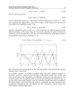
Fig. 9. Vibration signals when e xcited with voltage a t 120 Hz. in all sensors.
Fig. 10. Vibration signals when excited with voltage at sensor 2 in all frequencies.
axis represents each one of the ten (or twelve) repetitions of each experiment with the same
operational condition.
Figure 7 shows the vibration signals when excited with current at 120 Hertz in all sensors.
Notice that the steps shown in the figure correspond to excitations of 30% of the nominal
current (lower amplitudes) and then 60%, 100% and 120%. Figure 8 shows the vibration
signals captured at sensor 2 in all the frequencies of the same experiment. Notice that the
amplitude of the vibration increases when current increases. Notice also that the frequencies
of 120 and 240 Hertz are the only representatives of the vibrations compared to other multiples
of 60 He rtz.
Figures 9 and 10 show the experiments with voltage and no current. Figure 9 shows the
vibration signals at 120 Hetrz in all sensors, and Fig. 10 shows the vi bration at sensor 2 in all
frequencies.
These graphs are examples of the kind of variations that we found in the vibrational pattern,
under different operational conditions.
115

Probabilistic Vibration Models in the Diagnosis of Power Transformers
14 Vibration Analysis
Following the transformation of the vibration signals in their frequency components, a
normalization procedure is applied. Normalization in this context means that all variable
values lie between 0 and 1. This is because we only need to compare the behavior between all
the vibration signals. The normalization is obtained dividing all the vibration signals by t he
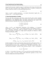
highest measure of each sensor. Figure 11 shows an example of normalized signals. Notice
that all signals detected at a ll sensors b ehave similar even if their amplitude are different as
was shown in Fig. 7.
Fig. 11. Comparison between the behavior of al l the signals when normalized.
Finally, a discretization is required since the probabilistic model utilizes Bayesian networks
with discrete signals. Discretization is the division of the complete range of values in a fixed
number of intervals. In our experiments, the vibration signals were discretized in 20 intervals
or states S
0
, S
1
, ,S
19
. Since no rmalized, the states consists in 5% of the normalized signals,
i.e., 0
− 0.05, 0.05 − 0.1 and so on .
Table 3 resumes the variables utilized in the diagnosis and the values that they can take.
Variable Values
Temperature Cold, hot
Excitation Voltage, Current
Nominal Voltage 70%, 80%, 90%, 100%, 110%
Nominal Current 30%, 60%, 100%, 120%
Sensors A1,A2, ,A8
Frequencies 60Hz.,120Hz.,180Hz., ,900Hz., 960Hz.

Table 3. Variables utilized in the diagnosis.
The next section utilized these variables to build the probabilistic models.
4.2 Model of correct transformers
In the first stage of this project, the variables available for constructing the model are sensors,
frequencies, temperature and excitation of the transformer (voltage or current). Following
the experts’ advice, we consider two possible set of models. The first is a model relating
116
Recent Advances in Vibrations Analysis
Probabilistic Vibration Models in the Diagnosis of Power Transformers 15
operational conditions and frequencies. One model for each sensor. The second possible set
of models relates operational conditions and sensors. One model for each frequency. We
decided to try a set of models that relates conditions and sensors, i .e, operational conditions
and vibrations detected in certain parts of the transformer. F igure 12 shows one instance of
the resulting model.



Fig. 12. Model that relates operational conditions with the amplitude measured by each
sensor.
Actually, the complete model is formed by two BNs like the one shown in Fig. 12. One
corresponding to the 120 Hz component and the second corresponding to 240 Hz. Once
defined the structure, the EM (Estimation-Maximization) algorithm (Lauritzen, 1995) is
utilized to obtain the conditional probability tables. We used 10 experiments of each type as
indicated in Table 2 and applied in 5 transformers. The structure and the parameter learned,
complete the models for the diagnosis. Next section describes the diagnosis procedure in the
factory floor.
4.3 Diagnosis procedure in FAT
Utilizing the models described above, the algorithm 1 is applied to identify abnormal
vibrations in the sensors given ce rtain operational conditions:
Algorithm 1 Detection of abnormal vibrations.

Require: Operational conditions of temperature and excitation.
assign a value (instantiate) to the temperature and excitation nodes
for all sensors (frequencies) in the network do
propagate probabilities and obtain a posterior probability of all sensors (frequencies)
nodes
compare the re al value measure and the estimated v alue
evaluate if there is an error in the s ensor (frequency)
end for
As an example, Table 4 s hows the measures that have been obtained and normalized in the
sensors of a cold transformer excited with 100% of nominal current.
Sensor 1 Sensor 2 Sensor 3 Sensor 4 Sensor 5 Sensor 6 Sensor 7 Sensor 8
0.3284 0.3710 0.0895 0.4161 0.0811 0.7084 0.6531 0.2333
Table 4. Example of vibration measured i n the sensors.
According to the algorithm 1, one sensor vibration is estimated using the rest of the sensor
signals and the operational conditions. The probabilistic propagation in the BN produces a
117
Probabilistic Vibration Models in the Diagnosis of Power Transformers
16 Vibration Analysis
posterior probability distribution of the estimated sensor value. The problem is to map the
observed value and the estimated value to a binary value: {correct, faulty}. For example,
Fig. 13 left shows an example of a posterior probability distribution, and Fig. 13 right shows
a wider distribution. In both cases, the observed value of the estimated sensor is shown by
an arrow. Intuitively, the first case can be mapped as correct while the second can be tak en as
erroneous.
Fig. 13. Example of two posterior probabilistic distributions and the comparison with the
value read.
In general, this decision can be made in a number of ways including the following.
1. Calculate the distance of the real value from the average or mean of the distribution, and
map it to faulty if it is beyond a specified distance and to correct if it is less than a specified
distance.

2. Assume that the sensor is working properly and establish a confidence level at which this
hypothesis can be rejected, in which case it can be considered faulty.
The first criterion can be implemented by estimating the mean μ and standard deviation σ of
the posterior probability of each sensor, i.e., the distribution that results after the propagation.
Then, a vibration can be assumed to be correct if it is in the range μ
± nσ,wheren = 1, 2, 3.
This criterion allows working with wider distributions where the standard deviation is high
and the real value is far from the mean μ value as shown in Fig. 13 right. However, this
technique can have problems when the highest probability is close to one, i.e., the standard
deviation is close to zero. In such situations, the real value must coincide with that interval.
The second criterion assumes as a null-hypothesis that the sensor is working properly. The
probability of obtaining the observed value given this null-hypothesis is then calculated.
If this value, known as the p-value (Cohen, 1995), is less than a specified level, then
the hypothesis is rejected and the sensor considered faulty. Both criteria were evaluated
experimentally. Here, it is worth mentioning that using the p-value witha0.01rejectionlevel,
works well.
4.4 Experiments for FAT
We designed a computational program that utilize the measurements obtained in the
experiments described in Table 2. We run experiments and identify if there is a failure.
An experiment consists in establishing the operational conditions of excitation and
temperature. Next, the system obtain the measurements of the sensors, and executes the
118
Recent Advances in Vibrations Analysis
Probabilistic Vibration Models in the Diagnosis of Power Transformers 17
algorithm for detection of abnormal vibrations. Since we have 16 indicators of fault (eight
sensors in two frequencies), a sensor fusion technique is required. We decided to make a
weighted sum of the conclusion of each sensor. If one sensor is sensible and detects deviations
easily, then a low weight is assigned. Other less sensible sensors may have higher weights.
Given the sum of each frequency, we can configure ranks for declare a transformer as {correct,
suspicious, faulty}.

Fig. 14. User interface of the diagnosis software (in S panish).
Figure 14 shows the results of one experiment (in Spanish). In the upper l eft of the window,
the operational conditions are indicated. First, load (carga en %) with 100% of current, and
cool tr ansformer temperature (frio). In the middle left of the window, there are two lights. O ne
corresponds to a model for 120 Hz. and the o ther corresponds to 240 Hz. As mentioned above,
we are using one model for each frequency. These lights become green if the transformer is
correct, yellow if the transformer is suspicious and red if there is definite a failure. Below, in
the lower left of the window, there are a little box for each sensor in the transformer. T he first
8 corresponding to 120Hz and the last corresponding to 240 Hz. If the posterior probability
obtained in a node ( sensor) corresponds to the vibrational value cur rently detected, then an
OK mark is described, and a NO-OK mark otherwise. Notice that the sixth sensor detected
a deviation in the model of 240 Hz. In the upper right of the window, four rows of data
are included. The first two correspond to the current vibration amplitude measured in the
8 sensors in the transformer. The next two ro ws correspond to the normalized information.
They are actually the inputs to the BNs. The lower right part of the window displays other
prototype information.
119
Probabilistic Vibration Models in the Diagnosis of Power Transformers
18 Vibration Analysis
Several transformers have been tested in factory and some faults have been detected. The next
section describes the changes made to the model in order to run SAT tests.
4.5 Preliminary experiments for SAT
Experiments in site have certain differences with FAT experiments. The main difference is that
transformers always operate at their fixed nominal voltage but variable current. The current
value corresponds t o the demanded power by the consumers.
In order to utilize the information acquired in FAT experiments, one assumption was
necessary: v ibration corresponds to the sum of vibration by current (produced at the winding)
plus vibration by fixed voltage at 100% of nominal value (produced at the core). This
assumption i s valid at the transformer operational condition below the saturation condition.

Voltage is always fixed at its nominal value (controlled b y the grid), and the current is always
tried to keep in normal conditions. In reality, we use all the information acquired for FAT
experiments, modified with this assumption.
Additionally, we run experiments in power transformers working on site. Of course, we could
not modify the working conditions and we took only data in certain loads.
Table 5 shows an example of the experiments carried out at the power transformer in Prolec
GE substation. The transformer provides power to the entire plant. Columns indicate the
measurement obtained by all every s ensor. The first row indicates the real amplitude o btained
by the sensor and normalized. Once normalized, the signals are discretized in 20 intervals.
The second row indicates the interval number, from 0 to 19. T hird row indicates the posterior
probability obtained after the propagation in the probabilistic model. This number indicates
the probability of being a normal measurement, so the fourth row decides if there is a failure
(1 value) or there is no failure (0 value). This decision is based on the assumption that the
posterior probability distribution is Gaussian given certain operational conditions. Thus, the
real value measured is compared with
±σ from the media.
S1 S2 S3 S4 S5 S6 S7 S8
Real value measured 0.159 0.121 0.184 0.178 0.083 0.016 0.729 0.141
Corresponding i nterval 3 2 3 3 1 0 14 2
Posterior probability 0.312 0.312 0.0 0.0 0.687 0. 0 0.0 0.375
Decision 0 0 1 0 0 0 1 0
Table 5. Example of one experiment.
For example in Table 5 , sensor 2 measured a normalized value of 0.121 that corresponds to
the interval number 2. Propagation indicates 31% of the value that corresponds to no failure.
On the contrary, sensor 7 reads a no rmalized value of 0.729, corresponding to interval 14 and
there is no probability of being correct. The decision is 1. Notice however, that sensor 6 has
the same 0 probability but the standard deviation may be very wide and the decision marked
0.
The prototype was constructed using the hugin platform (Andersen et al., 1989), so the off–line
automatic learning and the on–line propagation are carried out with the Java APIs of this

package.
Several tests were made in this Prolec GE substation transformer and the model resulted in a
correct tool for transformer diagnosis.
120
Recent Advances in Vibrations Analysis
Probabilistic Vibration Models in the Diagnosis of Power Transformers 19
5. Conclusions and future work
The main contribution of this work is the construction of a probabilistic vibration model
obtained with the vibration signals measured in a power transformer. Thus, if a model of
correct behavior can be obtained, then early deviations of this behavior can also be achieved.
Our approach utilizes Bayesian networks as the formalism for constructing and utilizing the
models. We used 8 sensors situated all around the tank of the transformer. Every measure
was transformed to the frequency domain and only amplitude multiples of the 60 Hz were
considered. Experiments were carried out at different operational conditions to construct the
models. Finally, a diagnosis program receives vibration data from a transformer, inserting it
as evidence and probability propagation allows calculating the probability of proper behavior.
Bayesian networks have the advantage of generate conclusions even when the evidence is
incomplete. This means that even with less sensors or less frequencies, a conclusion can be
obtained. Also, BNs include several algorithms that automatically adapt the models, based on
vibration in the normal life o f the transformer. This means we can detect the normal be havior
of old transformers even if they vibrate much more that their vibration when new.
Future work is needed in the determination of additional operation conditions variables, like
parameters in the construction of each transformer. We can detect the vibration transmission
between different parts of the transformer and identify more clearly if the behavior is normal
or not.
Final results will be available after months of tests in new and o ld transformers, in site and at
the factory.
6. Acknowledgments
This research is partially supported by Consorcio Xignux-Conacyt and by the Prolec GE-IIE
project 13261-A.

7. References
Andersen, S. K., Olesen, K. G., Jensen, F. V. & Jensen, F. (1989). Hugin: a shell for building
bayesian belief universes for expert systems, Proc. Eleventh Joint Conference on Artificial
Intelligence, IJCAI, Detroit, Michigan, U.S.A., pp. 1080–1085.
CFE (2010). Generación termoeléctrica, />Paginas/Indicadoresdegeneracion.aspx.
Cohen, P. (1995). Empirical methods for artificial intelligence, MIT press, Cambridge, Mass.
Crowley, T. H. (1990). Automated diagnosis of large power transformers using adaptive model-based
monitoring, Master of science in electrical engineering, Massachusetts Institute of
Technology, MIT, Boston, Mass., U.S.A.
García, B., Burgos, J. C. & Alonso, A. M. (2006a). Transformer tank vibration modeling as
a method of detecting winding deformations - part i: Theoretical foundation, IEEE
Transactions on Power Delivery 21(1): 157–163.
García, B., Burgos, J. C. & Alonso, A. M. (2006b). Transformer tank vibration modeling as a
method of detecting winding deformations - part ii: Experimental verification, IEEE
Transactions on Power Delivery 21(1): 164–169.
Golubev, A., Romashkov, A., Tsvetkov, V., Sokolov, V., Majakov, V., Capezio, O., Rojas, B.
& Rusov, V. (1999). On-line vibro-acustic alternative to the frequency response
121
Probabilistic Vibration Models in the Diagnosis of Power Transformers
20 Vibration Analysis
analysis and on-line partial discharge measurements on large power transformers,
Proc. TechCon Annu. Conference, TJ/H2b, Analytical Services Inc., New Orlans, L.A.,
U.S.A., pp. 155–171.
Harlow, J. H. (2007). Electric Power Transformer Engineering, CRC Press.
Lauritzen, S. L. (1995). The em algorithm for graphical association models with missing data,
Computational Statistics & Data Analysis 19: 191–201.
Lavalle, J. C . (1986). Failure detection in transformers using vibrational analysis, Master of science
in electrical engineering, Massachusetts Institute of Technology, MIT, Boston, Mass.,
U.S.A.
McCarthy, D. J. (1987). An adaptive model for vibrational monitoring of power transformers,

Master of science in electrical engineering, Massachusetts Institute of Technology,
MIT, Boston, Mass., U.S.A.
Neapolitan, R. (2004). Learning Bayesian Networks, Prentice Hall, New Jersey.
Pearl, J. (1988). Probabilistic reasoning in intelligent systems: networks of plausible inference,
Morgan Kaufmann, San Francisco, CA.
122
Recent Advances in Vibrations Analysis
7
Measurement of Satellite Solar Array
Panel Vibrations Caused by Thermal
Snap and Gas Jet Thruster Firing
Mitsushige Oda
1
, Yusuke Hagiwara
2
, Satoshi Suzuki
3
,
Toshiyuki Nakamura
1
, Noriyasu Inaba
1
, Hirotaka Sawada
1
,
Masahiro Yoshii
1
and Naoki Goto
1

1
Japan Aerospace Exploration Agency (JAXA)
2
Tokyo Institute of Technology
3
AES Co., Ltd
Japan
1. Introduction
Many space satellites have large solar array paddles (Fig. 1) for power generation and large
antennas for observation and communication. These large space structures are folded
during transport into space by launch vehicles, and deployed after arriving in space. The
paddles and antennas must be lightweight because of the payload weight limit of the launch
vehicle and are therefore very flexible, with little damping ability. This results in vibrations,
which cause serious problems. In particular, there have been increasing demands for
enhanced resolution of Earth observations from low Earth orbiting satellites in recent years.
Accordingly, the requirements for satellite attitude stability are also increasing. Conversely,
it is also known that the attitude stability of low Earth orbiting satellites is disturbed when
the satellites go into and leave an eclipse. When the thermal environment around a flexible
structure on orbit such as a solar array paddle changes to cold or hot, the flexible structure


Fig. 1. A solar array paddle in orbit © JAXA

Recent Advances in Vibrations Analysis

124
produces its own deformation or vibration. These occur most often during rapid
temperature changes called thermal snap or thermally-induced vibration, which has been
known to cause attitude disturbance in Low Earth Orbit (LEO) satellites.
Thermal snap vibration occurring on a flexible solar array panel is very slow, and measuring

motion on a solar array panel caused by thermal snap with sensors, such as an
accelerometer, is very difficult. The behaviour of a space structure affected by thermal snap
has never been observed directly in space until now. In this chapter, our vibration
measurement method, along with images taken in space and the image processing
conducted with the images taken on the ground, is explained, and some measurement
results are shown.
2. Thermal snap
Thermal snap is a unique phenomenon affecting flexible space structures and one of the main
factors causing disturbances in satellites. When a satellite enters an eclipse, the whole of the
solar array paddle or solar array panels are subject to rapid cooling, while the temperature of
the panel on the sun side is high beforehand. When the satellite leaves the eclipse, the sun side
of the solar array panels heats up rapidly, while the temperature difference between both sides
of the solar array panel is small when the satellite is in the eclipse.
These rapid changes of temperature difference between both sides of the solar array panels
result in thermal expansion and shrinking of the solar array panels and cause the solar array
panels to bend. This bending then, in turn, causes the solar array panels to vibrate and
results in degradation of the satellite attitude stability.
Many past satellites and space structures observed thermal snap from their attitude data.
The Hubble Space Telescope (HST) shown in Fig. 2 was launched by the space shuttle
Discovery on April 25, 1990, to conduct higher-accuracy astronomical observations than
ground-based equipment (Foster et al., 1995). A pointing control system of HST was
designed to hold an image stable at the HST focal plane to 0.007 arcsec (rms) for the
duration of an observation. However, following successful deployment of a pair of solar
array paddles, gyro data revealed significant attitude disturbances; observed when HST
entered or left the shadow of the earth. Based on investigation of HST’s telemetry data and
certain analyses, it was concluded that the disturbance of HST was caused by the thermally-
induced deformation of the HST solar array paddle. The HST solar array paddle has a
flexible solar array blanket and deploys a boom named the two-element Storable Tubular
Extendible Member (Bi-STEM). When HST remains in orbit on the day side, its deploying
boom heats up and a thermal gradient appears. The surface directed toward the Sun is

hotter than the opposite one and the thermal gradient also causes the solar array paddle to
bend. Conversely, when HST is in orbit on the night side, the whole of the boom cools down
and the thermal gradient disappears, while the bending of the solar array paddle is also
absent. This bending motion occurs rapidly during sunshine/eclipse transition and disrupts
HST’s pointing system. In December 1993, the space shuttle Endeavour was launched and the
solar array paddles were replaced with new units to counter the problem.
The Upper Atmosphere Research Satellite (UARS), launched in September 1991, and the
Advanced Land Observing Satellite (ALOS), launched in January 2006, in addition to HST,
also observed an attitude disturbance of the main body based on gyro telemetry data when
they traversed boundaries between the orbital day and night sides (Iwata et al., 2006;
Johnston & Thornton, 2000). However, these phenomena are rarely observed or measured
Measurement of Satellite Solar Array Panel Vibrations
Caused by Thermal Snap and Gas Jet Thruster Firing

125

Fig. 2. Hubble Space Telescope
directly since the solar array panel motions caused by thermal snap are very slow and
difficult to measure using sensors such as accelerometers. Additionally, the measurement
system has to be compact because of the strict payload limit, meaning there have been
hardly any direct measurements of thermal snap in orbit to date.
3. Measurement system using an onboard monitoring camera
This section introduces the equipment and configuration of our measurement system. To
measure vibration on flexible space structures, we proposed a method using a single
monitoring camera mounted on a satellite, the latter of which has several monitoring
cameras to monitor its own states. Our measurement system uses one of them, which
monitors solar array paddles.
3.1 GOSAT
Our measurement system is installed on JAXA’s (Japan Aerospace Exploration Agency)
Earth observation satellite named GOSAT (Greenhouse gases Observing Satellite), and

measures the deformation and vibration of its solar array paddle. GOSAT was launched on
January 2009. Its major parameters are shown in Table 1, and an overall view in Fig. 3.

Size
Main body
3.7 m (H)  1.8 m (W)  2.0 m (D)
Wingspan 13.7 m
Mass 1750 kg
Power 3.8 kW
Lifespan 5 years
Orbit
Sun Synchronous Orbit
Local time 13:00 ± 0:15
Attitude 666 km
Inclination 98 deg
Re-visit 3 days
Launch
Vehicle H-IIA
Schedule Jan. 2009
Table 1. GOSAT Summary

Recent Advances in Vibrations Analysis

126

Fig. 3. Overall view of GOSAT
GOSAT has eight CMOS cameras to monitor the deployment state of solar array paddles,
their post-deployment behaviour, the existence of contamination in the opening of fairing,
separation of the satellite from a launch vehicle, and so on. The effective sensor resolution of
the cameras is 1.3 million pixels. The monitoring camera which we used for monitoring the

whole of the solar array paddle thus has a short focal length and a wide view angle while
the monitoring camera we used for measurement is shown in Fig. 4 and has an LED lighting
system.


Fig. 4. Monitoring camera mounted on GOSAT © Meisei Electric Co., Ltd.
Measurement of Satellite Solar Array Panel Vibrations
Caused by Thermal Snap and Gas Jet Thruster Firing

127
3.2 Assumptions to measure the vibration
The solar array panel’s vibration is measured using one CMOS camera mounted on the
satellite main body. Since the images taken by a single CMOS camera do not include 3-D
information, some assumptions are needed to identify the vibration of the solar array
panels. The major assumptions are as follows:
3.2.1 Solar array panel
The GOSAT has a pair of solar array paddles, unlike most remote sensing satellites in low
Earth orbits, which have only one. This is to improve robustness against failures in the solar
array paddle, which resulted in the total loss of the ADEOS and ADEOS-II, which are
JAXA’s former remote sensing satellites. Each paddle consists of three semi-rigid panels and
a yoke. These solar panels were folded down to the satellite main body during the rocket
launch and released in orbit. During this measurement, we consider the solar paddle, which
comprises three panels, to be actually a single uniform panel. Fig. 5 shows the size of the
solar array paddle and its visual markers, namely about 2800  6000 mm.


Fig. 5. Size of the solar array paddle and its visual marker
3.2.2 Visual markers
The vibration of the solar array paddle caused by thermal snap occurs during poor lighting
conditions for the monitoring camera (eclipse). Additionally, the lighting condition changes

dramatically while the satellite goes from sunshine into the eclipse. Visual markers and an
LED lighting system are used to help Interference the motion of the solar array paddle. The
visual marker is made of reflective tape and is 50  26 mm in size. Unfortunately, these
markers are attached only to the front surface (solar cell side) of the solar paddle, to avoid
mechanical interface with the solar cell panels when they are folded down to the satellite
main body. Displacement of the solar array paddle can be obtained by measuring the
positions of the Visual markers.
3.2.3 Vibration modes
We assumed that the GOSAT’s solar array paddle has three major vibration modes as
shown in Fig. 6, namely out-of-plane vibrations, twists, and in-plane vibrations. Higher
order vibrations are not considered.

Recent Advances in Vibrations Analysis

128
Twist
In-plane vibration
Out-of-plane vibration

Fig. 6. Vibration modes of the solar array panel
3.3 Ground-based test model for the algorithm development
To develop the measurement system and algorithm, a ground-based test model comprising
a scale model (1/3 scale) of the solar cell paddle, a compatible CMOS camera and an LED
lighting system are developed. An artist’s image of the test bed is shown in Fig. 7, and that
of the solar array paddle taken by the ground-based test model is shown in Fig. 8.


Fig. 7. A ground-based test model to develop the measurement system
4. Development of a high-accuracy image processing algorithm
Images taken by the mounted camera are down-linked to the ground and subject to

processing to measure the position of the reflective markers. The algorithm for the image
processing is shown in this section. One problem when measuring thermal snap is that the
lighting condition changes dramatically during the measurement. To resolve this, the image
processing algorithm is adjusted to use the same algorithm for both sunshine and eclipse. A
ground-based test model was used to develop our measurement system.