Recent Advances in Vibrations Analysis Part 13 ppt
Bạn đang xem bản rút gọn của tài liệu. Xem và tải ngay bản đầy đủ của tài liệu tại đây (234.34 KB, 8 trang )
Stochastic Finite Element Method in Mechanical Vibration
229
1
2
2
2
1
1
2
n
tt
tt tt i
aa
i
i
aa
a
(34)
where,
tt
expresses the mean value of
tt
.
The variance of
tt
is given by
1
2
2
1
n
tt
tt i
i
i
aa
Var
a
(35)
The partial derivative of
tt
with respect to
i
a is given by
023
tt t t
tt t
iiiii
bbb
aaaaa
(36)
The partial derivative of
tt
with respect to
i
a
is given by
67
tt t t tt
ii i i
bb
aa a a
(37)
The partial derivative of Eq.36 with respect to
i
a
is given by
2
22
0
222
tt
tt t
iii
b
aaa
22
23
22
tt
ii
bb
aa
(38)
The partial derivative of Eq.37 with respect to
i
a is given by
22
22
tt t
ii
aa
22
67
22
ttt
ii
bb
aa
(39)
The mean value and variance of the displacement are obtained at time
11 3
2,3, ,titi n step-by-step.
The partial derivative of Eq.27 with respect to
i
a is given by
d
t
dd
tt
ii i i
DB
BD DB
aa a a
(40)
The partial derivative of Eq.40 with respect to
i
a is given by
2
2
22
d
t
ii
D
B
aa
22
d
t
d
t
ii i i
DB D
B
aa a a
2
2
2
d
t
d
t
ii
i
BB
DD
aa
a
Recent Advances in Vibrations Analysis
230
2
2
d
t
i
DB
a
(41)
The stress is expanded at mean value point
1
12
,,,,,
T
in
aaa a a by means of a Taylor
series. By taking the expectation operator for two sides of the above Eq.27, the mean of
stress is obtained as
1
2
2
2
1
1
2
n
i
aa
i
i
aa
a
(42)
where,
expresses the mean value of
.
The variance of
is given by
1
2
2
1
n
i
i
i
aa
Var
a
(43)
6. Numerical example
Figure 1 shows a four-bar linkage, or a crank and rocker mechanism. The establishment of
differential equation system can be found in literature 10
,11,12.The length of bar 1 is
0.075m, the length of bar 2 is 0.176m, the length of bar 3 is 0.29m,and the length of the bar 4
is0. 286m, the diameters of three bars are 0.02m. The torque T is 4Nm, the load F1 is 20sint
N. The three bars are made of steel and they are regarded as three elements. Considering the
boundary condition, there are 13 unit coordinates. Young’s modulus is regarded as a
random variable. For numerical calculation, the means of the Young’s modulus within the
three bars are .
11
210 .
2
Nm and the variances of the Young’s modulus are
11
10
24
Nm.
Figure 2 shows the mean of the displacement at unit coordinate 11. Unit coordinate 11 is the
deformation of the upper end of bar 3 in the vertical direction. The DSFEM simulates 1000
samples. The TSFEM produces an error of less than 0.5%. The CG produces an error of less
than 0.1%. Figure 3 shows the variance of the displacement at unit coordinate 11. TSFEM
produces an error of less than 1.0%. CG produces an error of less than 0.4%.Figure 4 shows
the mean of stress at the top of bar 3. The TSFEM produces an error of less than 0.85%.The
CG produces an error of less than 0.13%.Figure 5 shows the variance of stress at the top of
bar 3. The TSFEM produces an error of less than 1%. The CG produces an error of less than
0.3%.The results obtained by the CG method and the TSFEM are very close to that obtained
by the DSFEM. Table 1 indicates the comparison of CPU time when the mechanism has
operated for six seconds.
Figure 6 shows a cantilever beam. The length, the width, the height , the Poisson’s ratio ,the
Young’s modulus and the load F are assumed to be random variables. Their means are 1m,
0.1m, 0.05m, 0.2,
11
210
2
Nm ,100N.Their standard deviation are 0.2, 0.1, 0.1, 0.01,
9
10
,
0.1. Load subjected to the cantilever beam is Fsin(100t)N. It is divided into 400 rectangle
elements that have 505 nodes. Figure 7 shows the mean of vertical displacement at node 505.
DSFEM simulates 100 samples. The result obtained by the TSFEM produces an error of less
than 2% . CG produces an error of less than 0.5%. Figure 8 shows the variance of vertical
Stochastic Finite Element Method in Mechanical Vibration
231
displacement at node 505.The TSFEM produces an error of less than 3.0%. CG produces an
error of less than 0.8%.Figure 9 shows the mean of horizontal stress at node 5. The TSFEM
produces an error of less than 2.4%. CG produces an error of less than 0.9%. Figure 10 shows
the variance of horizontal stress at node 5. The TSFEM produces an error of less than 3.2%.
CG produces an error of less than 1.3%. Table 2 indicates the comparison of CPU time when
the cantilever beam has operated for six seconds.
Fig. 1. A four-bar linkage
Fig. 2. The mean of displacement at unit coordinate 11 for
211
10
E
Recent Advances in Vibrations Analysis
232
Fig. 3. The variance of displacement at unit coordinate 11 for
211
10
E
Fig. 4. The mean of stress at the top of bar 3 for
211
10
E
Stochastic Finite Element Method in Mechanical Vibration
233
Fig. 5. The variance of stress at the top of bar 3 for
211
10
E
DSFEM TSFEM CG
19 seconds 4 seconds 14 seconds
Table 1. Comparison of CPU time for
211
10
E
Fig. 6. A cantilever beam
Recent Advances in Vibrations Analysis
234
Fig. 7. The mean of vertical displacement at node 505
Fig. 8. The variance of vertical displacement at node 505
Stochastic Finite Element Method in Mechanical Vibration
235
Fig. 9. The mean of horizontal stress at node 5
Fig. 10. The variance of horizontal stress at node 5
DSFEM TSFEM CG
3 hours 8 minutes 17 seconds 1 hour 45 minutes 10 seconds 40 minutes 24 seconds
Table 2. Comparison of CPU time
Recent Advances in Vibrations Analysis
236
7. Conclusions
Considering the influence of random factors, the mechanical vibration in a linear system is
presented by using the TSFEM. Different samples of random variables are simulated. The
combination of CG method and Monte Carlo method makes it become an effective method
for analyzing the vibration problem with the characteristics of high accuracy and quick
convergence.
8. References
[1] J. Astill, C. J. Nosseir and M. Shinozuka. Impact loading on structures with random
properties.J. Struct. Mech.,1(1972) 63-67
[2]
F. Yamazaki , M. Shinozuka and G. Dasgupta Neumann expansion for stochastic finite
element analysis. J. Engng. Mech. ASCE. 114 (1988):1335-1354
[3]
M. Papadrakakis and V. Papadopoulos. Robust and efficient methods for stochastic
finite element analysis using Monte Carlo Simulation. Comput. Methods Appl.
Mech. Engrg. 134(1996)325 -340
[4]
G. B. Baecher and T. S. Ingra. Stochastic FEM in settlement predictions. J. Geotech.
Engrg. Div.107 (1981)449-463.
[5]
K. Handa and K. Andersson. Application of finite element methods in the statistical
analysis of structures. Proc. 3rd Int. Conf. Struct. Safety and Reliability, Trondheim,
Norway (1981)409 -417.
[6]
T. Hisada and S. Nakagiri. Role of the stochastic finite elenent method in structural
safety and reliability. Proc. 4th Int. Conf. Struct. Safety and Reliability ,Kobe,
Japan(1985)385-394.
[7]
S. Mahadevan and S. Mehta. Dynamic reliability of large frames. Computers &
Structures 47 (1993)57-67.
[8]
W. K. Liu, T. Belytschko and A. Mani. Probabilistic finite elements for nonlinear
structural dynamics. Comput.Methods Appl. Mech. Engrg. 57(1986)61-81.
[9]
S.Chakraborty and S.S.Dey. A stochastic finite element dynamic analysis of structures
with uncertain parameters. Int. J. Mech. Sci. 40 (1998)1071-1087.
[10]
A.G.,Erdman and G.N.,Sandor.A general method for kineto-elastodynamic analysis and
synthesis of mechanisms.ASME, Journal of Engineering for Industry 94(1972) 1193-
1205.
[11]
R.C.Winfrey.Elastic link mechanism dynamics.ASME, Journal of Engineering for
Industry 93(1971)268-272.
[12]
D.A.,Turcic and A.Midha.Generalized equations of Motion for the dynamic analysis of
elastic mechanism system. ASME Journal of Dynamic Systems, Measurement ,and
,Control 106(1984)243-248.
[13]
M.Kaminski . Stochastic pertubation approach to engineering structure vibrations by
the finite difference method . Journal of Sound and Vibration (2002)251(4), 651—
670.
[14]
Kaminski,M.On stochastic finite element method for linear elastostatics by the
Taylor expansion Structural and multidisciplinary optimization 35(2008),213-223.
[15]
Sachin K;Sachdeva;Prasanth B;Nair;Andy J;Keane.Comparative study of projection
schemes for stochastic finite element analysis. Comput. Methods Appl. Mech.
Engrg. 195(2006),2371-2392.
[16]
Marcin Kaminski.Generalized perturbation-based stochastic finite element in
elastostatics. Computer
&structures.85 (2007),586-594.


