Risk Management in Environment Production and Economy Part 10 ppt

A Comprehensive Risk Management
Framework for Approaching the Return on Security Investment (ROSI)

169
In the sequence, to meet the goal of the chapter, section 4 presented as proposal a
comprehensive RM framework, extending the traditional approaches in two phases clearly
stated: planning and monitoring of ROSI (phase 3); and closing or extinction of the IT
environment resulting in the archiving or discarding activities within the system (Phase 5 -
aligned to the SDLC addressed in NIST SP 800-21 (NIST SP800-21, 2005)). Finally, section 5
has shown an analysis of ROSI application in RM, including:

Key Benefits:

ROSI adds a deeper financial analysis phase in the selection of controls, incorporating
criteria such as loss of productivity, business organizational interruption, loss of
intangible assets, depreciation, devaluation, reconstruction, recovery, monitoring of
investment compensation in a control etc;

ROSI allows to potentiate the saving of investments and cost-effectiveness for the
controls;

With the collection of measures (metrics) associated with the controls, it is possible to
verify if the planning done for a given control will be fulfill or not;

Major limitations:

ROSI generates savings, but neither revenue nor dividends arise from the invested
financial value;

ROSI brings up an additional work phase on the traditional risk management model,
therefore making this framework more complex and quantitative;


ROSI is based on events or incidents have occurred in the past or on the notion of the
current protection level for an IT environment, thus it is not possible to assess the future
trend of the attacks to verify if the investment compensation can occur in the short,
medium or long term.
The following future works may be suggested: an experimental analysis of ROSI approaches
applied in IT environments; to use forecasting techniques to know the behavior and volume
of the security attacks, thus helping to verify if the planning done for the ROSI will be
confirmed before or after the defined deadline; to prepare a formal proposal for the
implementation of ROSI taking into account the life cycle of IT systems; among others.
7. References
Al-Humaigani, M.; Dunn, D.B., A model of Return on Investment for Information Systems
Security,
Proceeding of 2003 IEEE International Symposium on Micro-NanoMechatronics
and Human Science, pp. 483, ISBN 0-7803-8294-3, Cairo, 2003.
Cavusoglu, H., Mishra, B., Raghunathan, S., A Model of Return on Investment for
Information Systems Security, (2004),
Journal Communications of the ACM, Volume
47 Issue 7, July 2004, ACM New York, NY, USA.
DARPA, Defense Advanced Research Projects Agency, DARPA, (1998), Massachusetts
Institute of Technology (MIT) - Lincoln Laboratory, 1998, Available from
/>.html.
Haslum, K, Abraham, A., Knapskog, S., Fuzzy Online Risk Assessment for Distributed
Intrusion Prediction and Prevention Systems,
Proceedings of IEEE UKSIM 2008 10th
International Conference on Computer Modeling and Simulation, pp. 216, ISBN 0-7695-
3114-8, Cambridge, UK, April 2008.

Risk Management in Environment, Production and Economy

170
IC3 - Internet Crime Complaint Center, (2008), 2008 Internet Crime Report, Bureau of Justice
Assistance and National White Collar Crime Center, 2008, Available from:
www.ic3.org.
ISO 13335, International Standardization Organization, ISO/IEC TR 13335. Information
Technology – Guidelines for the management of IT Security – part 1: Concepts and
Models for IT Security, Geneva, 2004.
ISO 27001, International Standardization Organization, ISO/IEC 27001. Information
technology Security techniques Specification for an Information Security
Management System, Geneva, 2006.
ISO 27002, International Standardization Organization, ISO/IEC 27002. Information
technology Security techniques Code of Practice for Information Security
Management, Geneva, 2005.
ISO 27005, International Standardization Organization, ISO/IEC 27005. Information technology -
- Security techniques Information security risk management, Geneva, 2008.
ISO 31000, International Standardization Organization, ISO/IEC 31000. Risk management —
Guidelines on principles and implementation of risk management, Geneva, 2009.
ISO 73, International Standardization Organization, ISO/IEC Guide 73. Risk management
Risk Management Vocabulary, Geneva, 2009, Geneva, 2009.
NIST SP800-21, National Institute of Standards and Technology, (2005), Guideline to
Implement Cryptograph in the Federal Government, USA, 2005.
NIST SP 800-30, National Institute of Standards and Technology, (2002), Risk Management
Guide for Information Technology Systems, USA. 2002
NIST SP 800-37, National Institute of Standards and Technology, (2010), Guide for Applying
the Risk Management Framework to Federal Information Systems, USA, 2010
PMBOK, Project Management Institute, (2008), PMBOK – Project Management Body of
Knowledge, A Guide to the Project Management Body of Knowledge, Forth
Edition, Paperback, PMI, December, 2008.
Pontes, E. & Geulfi, A., (2009), IDS 3G - Third Generation for Intrusion Detection: Applying
Forecasts and ROSI to Cope With Unwanted Traffic,

Proceedings of 2009 4th IEEE
ICITST International Conference for Internet Technology and Secured Transactions, pp. 1,
ISBN 978-1-4244-5647-5, London, UK, November 2009.
Pontes, E. & Guelfi, IFS — Intrusion Forecasting System Based on Collaborative
Architecture,
Proceedings of 2009 4th IEEE ICDIM International Conference on Digital
Information Management, pp. 1-8, ISBN 978-1-4244-4253-9, University of Michigan,
Ann Arbor, USA, November 2009.
Pontes, E. & Zucchi, W., (2010) Fibonacci Sequence and EWMA for Intrusion Forecasting
System,
Proceedings of 2010 5th IEEE ICDIM International Conference on Digital
Information Management, pp. 404-412, ISBN 978-1-4244-7572-8, Lakehead University,
Thunder Bay, Ontario, Canada, July 2010.
Pontes, E., Guelfi, A. & Alonso, E., (2009), Forecasting for Return on Security Information
Investment: New Approach on Trends in Intrusion Detection and Unwanted
Traffic,
Journal IEEE Latin America Transactions, Vol. 7, Issue 4, (December 2009), pp.
438-446, ISSN 1548-0992, São Paulo, Brazil.
SNORT, 2009, Available from .
United States Government, (2002), Federal Information Security Management Act of 2002 -
FISMA, USA, Dec. 2002, Available from:
W. Sonnenreich, , J. Albanese, and B. Stout, (2006), A practical approach to return on
security investment,
Journal of Research and Practice in Information Technology, Vol.
38, No. 1, pp. 45-56, ISSN 1443-458X, Australia, February 2006.
8
Market Risk Management with
Stochastic Volatility Models
Per Solibakke
Molde University College, Specialized University in Logistics, Molde,

Norway
1. Introduction
Risk assessment and management have become progressively more important for
enterprises in the last few decades. Investors diversify and find financial distress and
bankruptcy among enterprises not welcome but expected in their portfolios. Some
enterprises do extremely well and keep expected profits (and realised) at a satisfactory level
above risk free rates. In contrast, corporations should be run at its shareholders best interest
inducing project acceptance with internal rates of return greater than the risk adjusted cost
of capital. These considerations are at the heart of modern financial theories. However, often
not stressed enough, for the survival of a corporation financial distress and bankruptcy costs
can be disastrous for continued operations. Every corporation has an incentive to manage
their risks prudently so that the probability of bankruptcy is at a minimum. Risk reduction
is costly in terms of the resources required to implement an effective risk-management
program. Direct cost are transactions costs buying and selling forwards, futures, options and
swaps – and indirect costs in the form of managers’ time and expertise. In contrast, reducing
the likelihood of financial distress benefits the firm by also reducing the likelihood it will
experience the costs associated with this distress. Direct costs of distress include out-of-
pocket cash expenses that must be paid to third parties. Indirect costs are contracting costs
involving relationship with creditors, suppliers, and employees. For all enterprises, the
benefits of hedging must outweigh the cost. Moreover, due to a substantial fixed cost
element associated with these risk-management programs, small firms seem less likely to
assess risk than large firms
1
. In addition, closely held firms are more likely to assess risk
because owners have a greater proportion of their wealth invested in the firm and are less
diversified. Similarly, if managers are risk averse or share ownership increases
2
, the
enterprises are more likely to pursue risk management activities. Stringent actions from
regulators, municipal and state ownership and scale ownership (> 10-15%), may therefore

force corporations to work even harder to avoid large losses from litigations, business
disruptions, employee frauds, losses of main financial institutions, etc. leading to increased
probability for financial distress and bankruptcy costs.

1
See Booth, Smith, and Stolz (1984), DeMarzo and Duffie (1995), and Nance, Smith and Smithson (1993).
The improvements in use of information technology have made it more likely that smaller companies
use sophisticated risk-management techniques Moore et al. (2000).
2
Tufano (1996) finds that risk management activities increase as share ownership by managers
increases and activities decreases as option holdings increases (managerial incentives hypotheses).


Risk Management in Environment, Production and Economy
172
Energy as all other enterprises must take on risk if they are to survive and prosper. This
chapter describes parts of the portfolio of risks a European energy enterprise is currently
taking and describes risks it may plan to take in the future. The three main energy market
risks to be managed are financial, basis and operational risk. The financial risks are market,
credit and liquidity risks. For an energy company selling its production in the European
energy market, the most important risk factor is market risk, which is mainly price
movement risks in Euro (€). The credit risk is the risk of financial losses due to counterparty
defaults. The Enron scandal made companies to review credit policies. Finally, the liquidity
risk is market illiquidity which normally is measured by the bid-ask spread in the market. In
stressed market conditions the bid –ask spread can become large within a certain time
period. The next main risk category for energy companies is basis risk
3
which is risk of
losses due to an adverse move or breakdown of expected price differentials. Price
differentials may arise due to factors as weather conditions, political developments, physical

events or changes in regulations. Some markets operate with area prices that differ from the
reference prices and contract for differences (CfD) are established to allow for basis risk
management. The last main risk category is operational risk which is divided into legal,
operational and tax risks. Legal risks are related to non-enforceable contracts. Operational
risk is the risk of loss resulting from inadequate or failed internal processes, people, and
systems or from external events. Tax risk can occur when there are changes to taxation
regulations. Importantly, all these risks interrelate and affect one another making the use of
portfolio risk assessment and management relevant. Basis and operational risk measures
contribute to total relevant risk and some of the basis risk is related to market risk (CfDs). In
many ways, the key benefit of a risk management program is not the numbers that are
produced, but the process that energy companies go through producing the risk related
numbers.
Economic capital is defined as the amount of capital an energy corporation needs to absorb
losses over a certain time horizon (usually one year) with a certain confidence level. The
confidence level depends on the corporation’s objectives. Maintaining an AA credit rating
implies a one-year probability of default of about 0.03%. The confidence level should
therefore be 99.97%. For the measurement of economic capital the bottom up approach is
often used. In this method the loss distributions are estimated for different types of risks
(market and operational) over different business units and then aggregated. For an energy
corporation the loss distributions for market risks can be divided into for example price and
volume risk, basis risk into location and time risks and operational risks into business and
strategic risks (related to an energy company’s decision to enter new markets and develop
new products/line of business). A final risk aggregation procedure should produce a
probability distribution of total losses for the whole corporation. Using for example copulas,
each loss distribution is mapped on a percentile-to-percentile basis to a standard well-
behaved distribution. Correlation structures between the standard distributions are defined
and this indirectly defines correlation structures between the original distributions. In a
Gaussian copula the standard distributions are multivariate normal. An alternative is a
multivariate t distribution. The use of the t distribution leads to the joint probability of
extreme values of two or more variables being higher than in the Gaussian copula. When

many variables are involved, analysts often use a factor model:


2
1
ii i i
UaF aZ

   ,
where F and Z have standard normal distributions and Z
i
are uncorrelated with each other

3
Three components of basis risk: location basis (area supply/demand factors), time basis (grid
problems) and some mixed basis issues.

Market Risk Management with Stochastic Volatility Models
173
and uncorrelated with F. Energy corporations use both risk decomposition and risk
aggregation for management purposes. The first approach handles each risk separately
using appropriate instruments. The second approach relies on the power of diversification
of reducing risks.
The chapter is concerned with the ways market risk can be managed by European
enterprises. Several disastrous losses
4
would have been avoided if good risk management
practices had been enforced. The current financial crises may have been avoided if risk
management had reached a higher understanding at the level of the CEO and board of
directors. Normally, corporations should never undertake a trade strategy that they do not

understand. If a senior manager in a corporation does not understand a trading strategy
proposed by a subordinate, the trade should not be approved. Understanding means
instrument valuations. If a corporation does not have the in-house capability to value an
instrument, it should not trade it. The risks taken by traders, the models used, and the
amount of different types of business done should all be controlled, applying appropriate
internal controls. If well handled, the process can sensitize the board of directors, CEOs and
others to the importance of market, basis and operational risks and perhaps lead to them
thinking about them differently and aggregately.
2. Energy markets, financial market instruments and relevant hedging
The main participants in financial markets are households, enterprises and government
agencies. Surplus units provide funds and deficit units obtain funds selling securities, which
are certificates representing a claim on the issuer. Every financial market is established to
satisfy particular preferences. Money markets facilitate flow of short-term funds, while
those that facilitate flow of long-term funds are known as capital markets. Whether referring
to money market or capital market securities, the majority of transactions are pertained to
secondary markets (trading existing securities) and not primary markets (new issuances).
The most important characteristic of secondary markets is liquidity (the degree a security
can be liquidated without loss of value). If a market is illiquid, market participants may not
be able to find a willing buyer and may have to sell the security at a large discount just to
attract a buyer. Finally, we distinguish between organised markets (visible marketplace) and
the over-the-counter market (OTC), which is mainly a telecommunication network. All
market participants must decide which markets to use to achieve their goals or obtain
financing.
Europe’s power markets consist of more than half a dozen exchanges, most of which offer
trading in both spot, futures and option contracts, giving a dauntingly complex picture of
the markets. Moreover, the markets are fragmented along national lines. The commodity
itself is impossible to store, at least not on the necessary scale, and is subject to extreme
swings in supply and demand. And critical information about such key factors as the level
of physical generation is incomplete or not available at all in certain markets. The Nordic
market was one of the leaders on electricity liberalization, with Nord Pool becoming

Europe’s first international power exchange in 1996. Liquidity and volume have grown
significantly. Nord Pool trades and clears spot and financially settled futures in Finland,

4
Recent examples are Orange County in 1994 (US), Barings Bank (UK) (Zang, 1995), Long-Term Capital
Management (Dunbar, 2000), Enron counterparties, and several Norwegian municipals in 2007-2008.

Risk Management in Environment, Production and Economy
174
Sweden, Denmark and Norway, listing day and week futures, three seasonal forwards, a
yearly forward, contracts for difference and European-style options. Volume in its financial
power market in 2009 totaled 2,162 terawatt hours, valued at 68.5 billion euros. Cleared OTC
volumes in 2009 reached 942 TWh from 1,140 TWh in 2008. The European Energy Exchange
(EEX) in Germany is Europe’s fastest growing power futures market. EEX offers trading in
physically-settled German and French power futures as well as cash-settled futures based
on an index of power prices. On 1st April 2009, the Powernext SA futures activity was
entrusted to EEX Power Derivatives AG. The exchange also offers trading in German,
Austrian, French and Swiss spot power contracts, emission allowances and coal, and
launched trading in natural gas in 2009/2010. On 1st January 2009, Powernext
SA transferred its electricity spot market to EPEX Spot SE and on 1st September 2009 EPEX
Spot merged with EEX Power Spot. The exchange has more than 160 members from 19
countries, including banks such as Barclays, Deutsche Bank, Lehman Brothers and Merrill
Lynch. Eurex owns 23% of the exchange and supplies its trading platform. In 2009 the
volume of futures traded on EEX was 1,025 TWh, and the value of futures trading was 61
billion euros. The number of transdactions at the end of 2009 was approximately 114,250.
France’s Powernext exchange was established in 2002 as a spot market for electricity.
Futures trading were launched in 2004 and until 2009 traded physically-settled contracts
with maturities from three months to three years. In 2009 the exchange entrusted the futures
activity to EEX Power Derivatives AG. Moreover, 1st January 2009, Powernext SA
transferred its electricity spot market to EPEX Spot SE and on 1st September 2009 EPEX Spot

merged with EEX Power Spot. The transfer of activity was due to the implementation of
France’s TRTAM “return to tariff” law, which reinstates regulated tariffs for industrial users
from EDF, France’s main electricity supplier, which limits competition and is seen to distort
exchange prices. Liquidity was severely dented and trading volume plunged and open
interest sank from around 14 TWh in June 2006 to 11 TWh at the end of 2005. The European
Energy Derivatives Exchange (Endex) is funded by financial players and Benelux energy
market participants, including Fortis Bank, Endesa and RWE. It incorporates the Endex
Futures Exchange, an electronic market for Dutch and Belgian power futures, and Dutch gas
futures. Electrabel, Essent and NUON act as liquidity providers. Since the exchange
launched in 2004 the major interest has been in Dutch power futures, though Belgian power
markets have also grown. Combined, they rose 156% in year one and grew from 327 TWh in
2008 to 412 TWh in 2009. Number of transactions in Dutch power for 2009 was 45,900. In
November 2009, the Endex and Nord Pool take the first steps towards a integrated cross-
border intra-day electricity market. There are many other markets changing rapidly, or
where futures markets may develop. The U.K., for instance, is currently building a new
trading model to combat declining liquidity. A considerable amount of spot and forward
trading takes place on APX Power UK, but all attempts to create a futures market for U.K.
electricity have failed to attract significant volume. Most market participants have relied
instead on bilateral contracts traded on the over-the-counter market. The latest initiative is
Nord Pool and the N2EX market initiative started in 2009/2010. Volume is still an issue also
for this initiative. European markets are moving towards greater physical integration, with
more market coupling to increase the efficiency of cross-border interconnectors. Coupling
between Denmark and Germany is due, with EEX and Nord Pool party to an existing
agreement. Similarly, the 700MW NorNed interconnector links the Dutch APX market with
Nord Pool via Norway. The future could well see consolidation among exchanges,
particularly as cross-border integration becomes more widespread.

Market Risk Management with Stochastic Volatility Models
175

Table 1. Volume (TWh) and Number of Transactions for European Power markets
A financial futures contract is a standardised agreement to deliver or receive a specified
amount of a specified financial instrument at a specified price and date. The instruments are
traded on organised exchanges, which establish and enforce rules of trading. Futures
exchanges provide an organised market place where contracts are traded. The marketplaces
clear, settle, and guarantee all transactions that occur on their exchange. All exchanges are
regulated and all financial future contracts must be approved and regulations imposed
before listing, to prevent unfair trading practices. The financial future contracts are traded
either to speculate on prices of securities or to hedge existing exposure to security price
movements. The obvious function of commodity future markets is to facilitate the
reallocation of the exposure to commodity price risk among market participants. However,
commodity future prices also play a major informational role for producers, distributors,
and consumers of commodities who must decide how much to sell (or consume) now and
how much to store for the future. By providing a means to hedge the price risk associated
with the storing of a commodity, futures contracts make it possible to separate the decision
of whether to physically store a commodity from the decision to have financial exposure to
its price changes. For example, suppose it is Wednesday week 9 and a hydro electricity
producer has to decide whether to produce his 10 MW maximum capacity of electricity from
his water reservoir, which has a normal level for the time of year, next week at an uncertain
spot price of S
1
or selling short a future contract to day at
1
0
F
. By selling the future contract,
the producer has obtained complete certainty about the price he will receive for his energy
production. Anyone using a future contract to reduce risk is a hedger. But much of the
trading of futures contracts are carried on by speculators, who take positions in the market

based on their forecasts of the future spot price. Hence, speculators typically gather
information to help them forecast prices, and then buy or sell futures contracts based on
those forecasts. There are at least two economic purposes served by the speculator. First,
commodity speculators who consistently succeed do so by correctly forecasting spot prices
and consequently their activity makes future prices better predictors of the direction of
change of spot prices. Second, speculators take then opposite site of a hedger’s trade when
other hedgers cannot readily be found to do so. The activity makes futures markets more
liquid than they otherwise would be. Finally, future prices can provide information about
investor expectations of spot prices in the future. The reasoning is that the future prices
reflects what inspectors expect the spot price to be at the contract delivery date and,
therefore, one should be able to retrieve that expected future spot price. Options are broader
class securities called contingent claims. A contingent claim is any security whose future
Power Futures (TWh) Carbon Trading (tonnes) Spot Power (TWh) Cleared OTC power (TWh)
2008 2009 2008 2009 2008 2009 2008 2009
Nord Pool Volume (TWh) 1437 1220 121731 45765 298 286 1140 942
Transactions 158815 136030 6685 3792 70 % 72 % 51575 40328
EEX Volume (TWh) 1165 1025 80084 23642 154 203 n/a n/a
Transactions 128750 114250 4398 1959 54 % 56 % n/a n/a
Powernext Volume (TWh) 79 87 n/a n/a 203.7 196.3 n/a n/a
Transactions n/a n/a n/a n/a n/a n/a n/a n/a
APX/Endex Volume (TWh) 327 412 n/a n/a n/a n/a n/a n/a
Transactions 36150 45900 n/a n/a n/a n/a n/a n/a
* On 1st January 2009, Powernext SA transferred its electricity spot market to EPEX Spot SE and
on 1st September 2009 EEX Power Spot merged with EPEX Spot.
* On 1st April 2009, the Powernext SA futures activity was entrusted to EEX Power Derivatives AG.

Risk Management in Environment, Production and Economy
176
payoff is contingent on the outcome of some uncertain event. Commodity options are traded
both on and off organised exchanges all around the world. Therefore, any contract that gives

one if the contracting parties the right to buy or sell a commodity at a pre-specified exercise
price is an option. European Energy Enterprises are all able to trade these securities on
organised exchanges and OTC markets. Traders and portfolio managers use each of the
“Greek Letters” or simply the Greeks, to measure a different aspect of the risk in a trading
position. Greeks are recalculated daily and exceeded risk limits require immediate actions.
Moreover, delta neutrality (

= 0) is maintained on a daily basis rebalancing portfolios
5
. To
use the delta concept, obtain delta neutrality and managing risks can be shown assuming a
electricity market portfolio for company TK AS in Table 2. One way of managing the risk is
to revalue the portfolio assuming a small increase in the spot electricity price from €65.27
per MW to €65.37 per MW. Let us assume that the new value of the portfolio is €65395. A
€0.1 increase in price decreases the value of the portfolio by €1000.


Table 2. Portfolio of Electricity Products in TK AS trading book (daily)
The sensitivity of the portfolio to the price of electricity is the delta:
1000
10000
0.1




.
Hence, the portfolio loses (gains) value at a rate of €10000 per €1 increase (decrease) in the
spot price of electricity. Elimination of the risk is to buy for example an extra one year
(month) forward contract for 10000/8250h (10000/740h) MW. The forward contracts gains

(loses) value of €10000 per €1 increase in the electricity price. The other “Greek letter” are
the Gamma
2
ortfolio








2
P
S
, Vega
ortfolio








P
, Theta
2
ortfolio
T









P
, and Rho
2
ortfolio








P
i
. Corporations in any market must distinguish between market, basis
and operational risk. The relevant risk is the market risk and the other risks are those over

5
Gamma and Vega neutrality on regular basis is in most cases not feasible.
Portfolio of Electricity Products in Tafjord Kraft book (daily):
Number of MW (000) Spot Prices (€) Value € (000)
Spot position (long normal production): 1000 65.27 65270

Forward contracts
One Year Forward Contracts -100 52.5 -5250
One Quarter Forward Contracts 50 68.23 3411.5
Two Quarter Forward Contracts -200 52.5 -10500
Four Quarter Forward Contracts 150 75.7 11355
One Month Forward Contracts 50 64.55 3227.5
Three Month Forward Contracts -10 58.25 -582.5
Future Contracts
One Week Future Contracts 100 67.25 6725
Two Weeks Future Contracts -50 65.21 -3260.5
Options
Call One Year Forward Options -10000
Put One Year Forward Options 5000
Total value of Portfolio Electricity 65396

Market Risk Management with Stochastic Volatility Models
177
which the company has control
6
(internal risk). In classical corporate finance textbooks we
find the separation theorem (the separation of ownership and management), which
defines all relevant risk as the market (external) risk while all other risk (internal) is
diversified away building diversified portfolios. Hence, the trade-off between return
versus risk (higher expected returns for higher risks) for investors must be separated from
risk and return for corporations. For an investor the relevant risk is
(, )
j
m
RR


, which
divided by
m

for scaling purposes, defines the

measure (often interpreted as market
sensitivity). Investors are therefore compensated only for market (systematic) risk. All
other risks can be diversified away building asset portfolios
7
. For corporations the
assumptions of shareholder wealth maximization are imposed. Every investment project
with a positive net present value (
NPV) discounted with the risk adjusted cost of capital
using the Capital Asset Pricing Model (
CAPM ) approach
8
, should be accepted.
Operational (non-systematic) risk is irrelevant
9
. However, there are two important
arguments among more (in an imperfect world) that can be extended to apply for all risks;
that is, bankruptcy costs (product reputations, service products, accountants and lawyers)
and managerial performance. The bankruptcy costs can be disastrous for a corporation’s
continued operations. It makes therefore sense for a company that is operating in the best
interest of its shareholders to limit the probability of this value destruction occurring.
Managerial performance evaluates company performance that can be controlled by the
executives in the organisation. Idiosyncratic risks not possible to control by company
executives should therefore be controlled. Hence, limiting total risk may be considered a
reasonable strategy for a corporation. Many spectacular corporate failures can be traced to

CEOs who made large levered acquisitions that did not work out. Corporate survival is
therefore an important and legitimate objective, where both financing and investment
decisions should be taken so that the possibility of financial distress (bankruptcy costs) is
as low as possible. To limit the probability of possible destructive occurrences, energy
corporations monitor market risks (mainly the correlated price and volume risks), basis,
and operational risk. Even though a corporation manage its Greek letters (delta, gamma,
theta and vega) within certain limits, the corporation is not totally risk free. At any given
time, an energy corporation will have residual risk exposure to changes in hundreds or
even thousands of market variables such as interest rates, exchange rates, equity markets,
and other commodity market prices as oil, gas and coal prices. The volatility of one of
these market variables measures uncertainty about the future value of the variable.
Monitoring volatility to assess potential losses for the corporation is therefore crucial for
risk management.

6
All internal risks are included as for example the rogue trader risk and the risk of other sorts of
employee fraud.
7
The Arbitrage Pricing Theory (APT) extends the one-factor model (CAPM) to dependence of several
factors (Ross, 1976).
8
The CAPM was simultaneously and independently discovered by Lintner(1965), Mossin (1966), and
Sharpe(1964).
9
Some companies in an investor’s portfolio will go bankrupt, but others will do extremely well. The
overall result for the investor is satisfactory.


Risk Management in Environment, Production and Economy
178

3. Value at risk, expected shortfall, volatility, correlations and copulas
3.1 Value at risk and expected shortfall
Value at Risk (VaR) is an attempt to provide a single number that summarizes the total risk
in a portfolio. VaR is calculated from the probability distribution of gains during time
T and
is equal to minus the gain at the (100 –
X)th percentile of the distribution. Hence, if the gain
from a portfolio during six months is normally distributed with a mean of €1 million and a
standard deviation of €2 million, the properties from a normal distribution, the one-
percentile point of the distribution is 1 – 2.33 * 2 = €3.66 million. The VaR for this portfolio
with a time horizon of six months and confidence level of 99% is therefore €3.66 million.
However, the VaR measure has some incentive problems for traders. A measure with better
incentives encouraging diversification (Artzner et al., 1999) is expected shortfall also called
conditional VaR (CVaR). As for the VaR, the CVaR is a function of two parameters:
T (the
time horizon) and
X (the confidence interval). That is, the expected loss during time T,
conditional on the loss being less than the
Xth percentile of the distribution. Hence, if the X
= 1%,
T is one day, the CVaR is the average amount lost over 1 day assuming that the loss is
greater than the 1% percentile. The CVaR measure is a coherent risk measure while the VaR
is not coherent.
The marginal VaR/CVaR is the sensitivity of VaR/CVaR to the size of the
ith sub-portfolio
ii
VaR CVaR
and
xx






and is closely related to the capital asset pricing model’s beta (

). If a
sub-portfolio’s beta is high (low), its marginal VaR/CVaR will tend to be high (low). In fact,
if the marginal VaR/CVaR is negative, an increase of the weight of a particular sub-
portfolio, will reduce overall portfolio risk. Moreover, incremental VaR/CVaR is the
incremental effect on VaR/CVaR of the
ith sub-portfolio. An approximate formula of the ith
sub-portfolio is
ii
ii
VaR CVaR
xand x
xx





. Finally, using the Euler theorem:
1
N
i
i
i
VaR

VaR x
x






and
1
N
i
i
i
CVaR
CVaR x
x





where N is the number of sub-portfolios. The component
VaR/CVaR of the
ith portfolio is defined as
i
VaR
i
i
VaR

Cx
x



and
CVaR
ii
i
CVaR
Cx
x



.
Component VaR/CVaR is often used to allocate the total VaR/CVaR to subportfolios – or
even to individual traders.
Back-testing is procedures to test how well the VaR and CVaR measures would have
performed in the past and is therefore an important part of a risk management system.
Var/ CVaR back-testing is therefore used for reality checks and is normally easier to
perform the lower the confidence level. Test statistics for one and two-sided tests have been
proposed (Kupiec, 1995). Bunch test statistics (not independently distributed exceptions) are
also proposed in the literature (Christoffersen, 1998). Weaknesses in a model can be
indicated by percentage of exceptions or to the extent to which exceptions are bunched.
3.2 Volatility, Co-variances/correlations and copulas
Volatility and correlation modelling of financial markets combined with appropriate
forecasting techniques are important and wide-ranging topics. Volatility is defined as the

Market Risk Management with Stochastic Volatility Models

179
standard deviation of variable i’s return
,
,
,1
ln 100
it
it
it
P
y
P










per unit time (t-1, t), where
P
i,t
is the price of asset i at time t. Relative to time horizons, the uncertainty measured by the
standard deviation increases with the square root of time


t

. There are approximately
252 (trading) days (
t) per year. Volatility estimates can normally be obtained from two
alternative approaches. The first is directly from the Black & Scholes option pricing formula
(1973, 1976) (implied volatility) and the second is to estimate volatility from historical data
series and make conditional forecasts. Implied volatility estimates assume an actively traded
market for the derivatives and therefore an up-to-date price.

Observing the price in the market, the volatility can be estimated by use of a Newton-
Raphson technique. This technique’s

-measure is used extensively by market traders (the
vega-measure). However, risk management is largely based on historical volatilities. The
s
i
estimate of standard deviation of returns (y
i
) is:

2
,
1
1
1
n
iiti
t
syy
n











, where
i
y
is
the mean for asset
i of the
,it
y
and n is the number of periods. The s
i
variable is therefore an
estimate of
i
t

. It follows that

i
itself can be estimated as
ˆ
i


, where
ˆ
i
i
s
t


and the
standard error of this estimate can be shown to be approximately
ˆ
2
i
n

. A corporation that
has exposure to two different market variables will have gains and losses non-linearly
related to the correlation between the changes in the variables. The correlation coefficient (

)
between two variables
R
1
and R
2
, is defined as







 
12 1 2
12
ERR ER ER
SD R SD R




, where E()
denotes expected value and
SD() denotes standard deviation. As the covariance between R
1

and
R
2
can be defined as


12
ERR






12
ER ER
the correlation between R
1
and R
2
can be
written as


 
12
12
cov ,RR
SD R SD R



. Two variables are defined as statistically independent if
knowledge about one of them does not affect the probability distribution for the other. That
is, if




21 2
|fR R y fR
for all y, where f() is the probability density function. However,
a correlation coefficient of zero between two variables does not imply independence. The
correlation coefficient measures only linear dependence. There are many other ways in

which two variables can be related. For example, for the values of
R
1
normally encountered,
there is very little relation between
R
1
and R
2
. However extreme values of R
1
tend to lead to
extreme values
10
of R
2
. The marginal distribution of R
1
(sometimes also referred to as the
unconditional distribution) is its distribution assuming we know nothing about
R
2
and vice
versa. To define the joint distribution between
R
1
and R
2
, how can we make an assumption
about the correlation structure? If the marginal distributions are normal then the joint

10
The quote is: “During a crisis the correlations seem all to go to one”!

Risk Management in Environment, Production and Economy
180
distribution of the variables are bivariate normal
11.
In the bivariate normal case a correlation
structure can be defined. However, often there is no natural way to define a correlation
structure between two variables. It is here copulas come to our rescue. Regardless of
probability distribution shapes, copulas are tools providing a way of defining default
correlation structures between two or more variables. Copulas therefore have a number of
applications in risk assessment and management. Formally, a Gaussian copula can be
defined for the cumulative distributions of
R
1
and R
2
, named F
1
and F
2
, by mapping R
1
= r
1

to
U

1
= u
1
and R
2
= r
2
to U
2
= u
2
, where




11 1
Fr Nu
and




22 2
Fr Nu
and N is the
cumulative normal distribution function (Cherubini et al., 2004) This means




11
111222
,uNFr uNFr

  
 
and




11
11 1 22 2
,r F Nu r F Nu





. The variables U
1

and
U
2
are then assumed to be bivariate normally distributed. The key property of a general
copula is that it preserves the marginal distribution of
R
1
and R

2
while defining a correlation
structure between them. In addition to the Gaussian copula we also have the Student-t copula
(the tail correlation is higher in a bivariate
Student-t-distribution than that in a bivariate
normal distribution). For more than two variables a multivariate Gaussian copula can be
used. Alternatively, a factor model for the correlation structure between the
U
i
can be used:


2
1
ii i i
UaF aZ   where F and the Z
i
have standard normal distributions and the Z
i

are uncorrelated with each other and uncorrelated with F. Other distributions can be used to
obtain for example a Student-t distribution for U
i
(Demarta and McNeil, 2004). Copulas will
is this paper be used to apply a simple model for estimating the value at risk on a portfolio
of electricity accounts (households/firms) and to value credit derivatives and for the
calculation of economic capital.
To illustrate and implement these market risk management concepts for the European
energy markets, the Nord Pool and EEX energy markets are quite evolved and liquid
markets for energy in Scandinavia and central Europe, respectively. In both markets, prices

for energy are established seven days a week for the spot market and from Monday to
Friday (not holidays) for the front week/month futures/forwards contracts. Hence, to
establish the necessary concepts and define volatilities, co-variances and copulas fir these
markets we use the financial EEX and Nord Pool base and peak load prices from Monday to
Friday. We use all available prices from Monday to Friday for front week and front month
contracts in the two energy markets. The price series are shown in Figure 1 (note the change
in currency from NOK to Euro (€) for contracts with physical delivery after December 31
st

2005). Prices seem to move randomly over time for both markets and contracts and is clearly
non-stationary. The prices seem to show movements similar to other commodity markets
and Solibakke (2006) have shown that energy markets seem to exhibit similar features to
other markets. The EEX markets show a much higher frequency of price spikes and after
adjusting for NOK and Euro differences the EEX market seem to have higher peak prices
than the Nord Pool market. Due to the obvious non-stationary prices we calculate the
returns in percent (logs) and these return series will be the main objects of our
investigations.

11
There are many other ways in which two normally distributed variables can be dependent on each
other. There are similar assumptions for other marginal distributions.


Market Risk Management with Stochastic Volatility Models
181
When distributions from energy market time series are compared with the normal
distribution, fatter tails are observed (excess kurtosis). The standardized fourth moment is
much higher than the normal distribution postulates
12.
Hence, distributions with heavier

tails, such as Paretian and Levy are proposed in the international literature for modelling
price changes. Moreover, the time series from energy markets show sometimes too many
observations around their mean value and the tails show different characteristics at the
negative (left) side relative to the positive (right) side of the distribution. In particular, the
spikes at the EEX market may give some positive skewness to the EEX markets price
changes.



Fig. 1. Price series for Nord Pool and EEX. Nord Pool Front Week and Front Month (base).
EEX front Month (base load) and Front Month (peak load).

Uni-variate and bi-variate return characteristics, densities (frequency distribution, normal
distribution and the Epanechnikov kernel), volatilities and correlations for the Nord Pool
front Week and Month contracts and the EEX Front Month base and peak load contracts are
reported in Figure 2. For all the density plots (panel A-D) we distinguish three main
arguments: the middle, the tails, and the intermediate parts (between the middle and the
tails). When moving from a normal distribution to the heavy-tailed distribution, probability
mass shifts from the intermediate parts of the distribution to the tails and the middle. As a
consequence, small and large changes in a variable are more likely than they would be if a
normal distribution were assumed. Intermediate changes are less likely. The QQ-plots
confirm this non-normal story for all return distributions. The contract volatilities (panel E-F)
show clearly different shapes between Nord Pool and EEX. However, the products within
the same market show similar volatility patterns. The asymmetry (panel G-H) is much
clearer at EEX than at Nord Pool. In particular, the EEX market seems to exhibit much more

12
See the first studies of this feature: Mandelbrot (1963) and Fama (1963, 1965).

Risk Management in Environment, Production and Economy

182

A: Nord Pool Front Week

B: EEX Front Month (base load)



C: Nord Pool Front Month (base load)

D: EEX Front Month Peak Load




E: Nord Pool volatility clustering (conditional volatility)




F: EEX volatilit
y
clusterin
g
(conditional volatilit
y
)

Market Risk Management with Stochastic Volatility Models
183

G: Nord Pool Asymmetry Measures (conditional volatility)
H: EEX Asymmetry Measures (conditional volatility)

I: Nord Pool: Bivaraite Week-Month Densit
y
and Correlatio
n
J: EEX: Bivariate Months Density and Correlation
Fig. 2. Characteristics of Nord Pool and EEX Front Week/Month Forward/Future Contracts
Nord Pool (www.nordpool.no) and EEX (www.eex.de)
positive asymmetry, that is – higher volatility from positive than negative price changes. In
contrast, the Nord Pool week future contract report a low but significant negative
asymmetry, in line with equity markets where the asymmetry is well known under “the
leverage effect”. Finally, panels I-J in Figure 2 report the bi-variate relationships in the Nord
Pool and EEX markets. The distributions for the two markets show similar densities but
0.2
0.3
0.4
0.5
0.6
0.7
0.8
0.9
1
Nord Pool: Correlation Week - Month Contracts
0.6
0.7
0.8
0.9

1
EEX: Correlation Front Month - Base and Peak Load

Risk Management in Environment, Production and Economy
184
clearly different mean and standard deviations. The correlations seem at a higher level in
the Nord Pool bi-variate front week and month contracts relative to the EEX bi-variate front
month base and peak load contracts. However, in some time periods the correlations are as
low as 0.23/4 for the Nord Pool market. Generally, the correlation seems high between
financial instruments within the two energy markets.
The densities for the energy markets returns suggest heavy tail distributions that have
relative to the normal distribution, more probability mass in the tails and in the middle, and
less mass in the intermediate parts of the distribution. That is, small and large price changes
are more likely and intermediate changes are less likely, relative to a normal distribution.
An alternative to the normal distribution is the power law. The power law asserts that it is
approximately true that the value

of a variable has the property that, when x is large
()xKx




where K and

are constants. The extreme Power Law has been found
to be approximately true for variables at many and diverse applications. The equation is
useful when we use extreme value theory for risk management purposes and is valuable for
VaR and CVaR calculations. Extreme value theory can be used to improve VaR estimates
and to deal with situations where the VaR confidence level is very high. The theory provides

a way of smoothing and extrapolating the tails of an empirical distribution.
Gnedenko (1943) stated that, for a wide range of cumulative distributions F(x), the
distribution of
()()
()
1()
u
Fu
y
Fu
Fy
Fu



converges to a generalised Pareto distribution as the
threshold u is increased. The generalised Pareto distribution is defined with the formula
1
1
,
() 1 1
y
Gy








 


. The distribution has two parameters that have to be estimated
from the data set


. The

parameter is the shape parameter and determines the
heaviness of the tail of the distribution (a normal distribution has
0


). The parameter

is
the scale parameter. Estimating and


can be done with maximum likelihood methods.
We first differentiate the cumulative distribution function with respect to
y and obtain the
probability density function
1
1
,
1
() 1
y

gy










. We choose first u close to the 95%
percentile point of the empirical distribution. The focus is for observations x > u. We now
assume that there are
n
u
such observations and they are
(1 )
u
in


. The likelihood
function becomes:

1
1
1
1
1

u
n
i
t
u













. Finally maximize its logarithm:

1
1
1
1
ln 1
u
n
i
t
u


















. The probability that u
y


conditional on
u

is
,
1()G
y

 . The probability that

u

is 1 – F(u). The unconditional probability that
()xx u


is now


,
1()1 ( )Fu G x u






. If
n is the total number of observations, an

Market Risk Management with Stochastic Volatility Models
185
estimate of


1()Fu
calculated from the empirical data is
u
n
n

. The unconditional
probability that


is therefore

1
,
() 1 () 1
uu
xu
nn
ob x G x u
nn








    





Pr .
For the equivalence to the power law, set



and the equation reduces to
1
()
u
n
x
ob x
n








Pr so that the probability of the variable being greater than x is


(the power law) where
1
u
n
K
n












and
1


, implying that the
()ob x

Pr
is consistent
with the power law. To calculate the
VaR with a confidence level of q it is necessary to solve
the equation:
()FVaR q

. We now use
1
11
u
n
VaR u
q
n








 




so that

11
u
n
VaR u q
n





   


. Finally, the expected shortfall
13
(CVaR) becomes

1
VaR u
CVaR









.




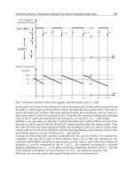
Fig. 3. The Power Law: Log plot for Electricity price increases:
x is the number of standard
deviations;

is the electricity price increase/decrease4. Stochastic volatility and risk
assessment/management

13
The choice of u does not influence the estimate of
()ob x

Pr
much. u should be approximately

equal to the 95
th
percentile of the empirical distribution.
-8
-7
-6
-5
-4
-3
-2
ln(prob(v < x))
Power Law for Nord Pool/EEX Front Week/Month Future/Forward Contracts
NP-Front-Week NP-Front-Month EEX Front Month (base load) EEX Front Month (peak load)

Risk Management in Environment, Production and Economy
186
A test of whether the power law
14
holds for the energy markets is to plot


()x



against ln
x. For the time series from the energy markets Nord Pool and EEX, define x as the
number of standard deviations by which electricity prices decreases in one day. Figure 3
shows that the logarithm of the probability of the electricity price decreasing by more than x
standard deviations is approximately linearly dependent on ln

x for x > 3. The power law
therefore seems to hold for energy market applications and we can therefore apply the
extreme value theory for VaR and CVaR calculations.
4. Stochastic volatility and risk assessment/management
4.1 The stochastic volatility model
The model building approach implies a need for a scientific model for the mean and
volatility using the MCMC (Markov Chained Monte Carlo) methodology to generate
distributions for
y=

P. A stochastic volatility (SV) model provide alternative models and
methodologies to EWMA and (G)ARCH models. SV models specify a process for volatility
and in the form used by Gallant et al. (1997) is formulated as:










01 10 1 2 1
1011,10 2
2012,10 3
11
2
2111 12
2

21 3 21 1 2
32
2
22
2321 1 3
exp( )
1
(( ))/1
1(())/1
tt ttt
ttt
ttt
tt
tt t
tt
t
t
yaay a v u
bb b u
cc c u
uz
usrz rz
rz r rr r z
us
rrrr r z







    
  
  




 




   



where
,1,2 3
it
zi and
are standard Gaussian random variables. The parameter vector is
01011012123
(,,,,,,,,,,)aabbsccsrrr


. The r
i
’s are correlation coefficients from a Cholesky
decomposition; enforcing an internally consistent variance/covariance matrix. Early

references are Rosenberg (1972), Clark (1973) and Taylor (1982) and Tauchen and Pitts
(1983). More recent references are Gallant, Hsieh, and Tauchen (1991, 1997), Andersen
(1994), and Durham (2003), see Shephard (2004) and Taylor (2005) for more background and
references. The model has three stochastic factor and extensions to four and more factors can
be easily implemented through the model setup. The inclusion of a Poisson distribution to
model jumps with the use of intensities, are applicable. Long memory can be formulated.
The long-memory stochastic volatility model can be described as

1
d
t
Lz




1t
u and
1
1
L
t
j
t
j
t
j
zazz







, valid for
|| 1/2d 
, as described by Sowell (1990). Other extensions

14
The power law can be rewritten as:


( ) ln lnxKx  
very useful for regressions and
the observing the possibility of empirically estimating ln K and  when the measure ln [Prob( > x)]
can be calculated.

Market Risk Management with Stochastic Volatility Models
187
of stochastic volatility models for better data fit are possible. Splines and t-errors have for
example been applied (Gallant and Tauchen, 1997). Liquid financial market normally
reports a much better model fit introducing three (or more) stochastic factors. The applicable
extensions will be called upon when needed.
Note that writing the variance rate (volatility) as:
22
1
1
1
m
ni

i
y
m





where
2
i
y
is observation i’s
squared return, is a particularly simple model for updating volatility estimates over time.
The Exponentially Weighted Moving Average (EWMA) model, where weights

decrease
exponentially as we move back through time (
1
,0 1
ii
 



) is such a simple model.
The formula becomes
15
:
22 2

11
(1 )
ii i
y
 


   
and can relatively easy be implemented
by using for example the Excel spreadsheet and the Solver routine. Adding a constant term
to this equation establish the (G)ARCH (generalised autoregressive conditional hetero-
scedastic) model. However, the number of EWMA/GARCH model reports/papers and the
simple fact that both methodologies have limited theoretical justifications, the chapter will
focus exclusively on the scientific SV model implementation for the Nord Pool and EEX
energy markets. In fact, it is only the SV-model estimation and simulation that makes a bi-
variate Nord Pool – EEX market density estimation possible. The SV-model implementation
use the computational methodology proposed by Gallant and McCulloch (2010) for
statistical analysis of a stochastic volatility model derived from a scientific process. The
scientific stochastic volatility model cannot generate likelihoods (latent variables) but it can
be easily simulated. The VaR can now be calculated as the appropriate percentile of the
distribution. The one-day 99.9% VaR for a 100
k simulation

P series is the value for the
100
th
-worst outcome. The 99.9% CVaR measure is the average of observations below the
99.9% percentile; that is, the average of the 100 observations.
4.2 The Nord Pool and EEX front week/month stochastic volatility models
The ( / )i NP Front Week Month

i,t
3644
y and the ( / )i EEX Front Month Base Peak Load
i,t
2189
y is
the percentage change (logarithmic) over a short time interval (day) of the price of a
financial asset traded on an active speculative market. The SV model implementation
established a mapping between a statistical model and a scientific model and the adjustment
for actual number of observations and number of simulation must be carefully logged for
final model assessment. For the SV model implementation reasonable starting values are
important. The implementation of the scientific model is a lengthy sequential process which
is finalized with a 25 CPU parallel computing run applying the Open-message passing
interface
16
(Open-MPI).

15
To understand why this equation corresponds to weights that decrease exponentially, substitute
2
1i


with
22
22
(1 )
ii
u
 



. The substitution produce:


2122
1
1
m
jm
ii
j
im
j
u
 




   

. For large
m the last term
2m
im
 is small enough to be ignored.
16
Open-MPI is a high-performance, freely available, open source implementation of the MPI standard
that is researched, developed, and maintained at the Open System Lab at Indiana University

(www.open-mpi.org).

Risk Management in Environment, Production and Economy
188
SV model extensions are condition specific. The extensions are analysed from both the score
model (
f
k
()) and from characteristics of the EMM implementation. The f
k
() indicates the
starting values and active SV model parameters for the EMM estimation. The normalised
scores quasi t-statistics indicate score failures and need for SV model extensions. Finally, the
Bayesian log posterior

2
test statistic and the Epanechnikov kernel density plots of
parameters and functional statistics (stats) assesses SV model optimality or fit. These
optimization routines together with an associated 25 iterative run for a comprehensive
model assessments, establish the empirical foundation of the Bayesian MCMC estimation
reports. The implementation of the 3x8-/2x12-core CPUs generates 240,000 simulated paths
for the stochastic volatility model. The Bayesian MCMC M-H algorithm

* optimal model
from the 24-core CPU parallel run model is reported in Table 3. The mode, mean and
standard errors are reported for the four series. For all models the optimal Bayesian log
posterior value is reported together with the

2
test statistic. Moreover, all the score

diagnostics (not reported) are all well below 2.0 in value
17.
The first important observation
from Table 3 is the four

2
(df) rejection statistics for the multifactor SV models. None of the
SV models are rejected at the 5% significance level. Moreover, the model diagnostics do not
identify score moments that are rejected (> 2). The SV models are therefore found accepted
for extended commodity market analyses. Table 3 suggests some important differences
between Nord Pool and EEX. The Nord Pool week contracts show the largest negative drift,
inducing a positive risk premium that is traded the last week before contract maturity. The
three other monthly forward products show all lower but negative drift. The volatility
seems highest for the Nord Pool week contracts (which also have the shortest time to
maturity)
18
. Finally, the analysis shows interesting mean – volatility correlation structures
for the EEX market. The asymmetry is found for both volatility factors. The first factor
report a positive asymmetry (largest) and the second volatility factor reports a negative
factor. From the initial plots in Figure 2, the positive factor seems to dominate asymmetry
for EEX. For the Nord Pool the correlation structure seems close to zero and insignificant.
That is, asymmetry and non-linearity seems higher for the EEX market than for Nord Pool,
which is close to negligible.
The multi-equation SV model reported in Table 3 can now be easily simulated at any length.
First, Figure 4 reports plot of standard deviation versus returns for the original series with
3644 observations for Nord Pool (left: panel A and B) and 2189 observations for EEX (right:
panel C and D) in the upper part of the figures and a simulated series with 100
k
observations right below. From these plots we can find signs of positive volatility
asymmetry for the EEX market, while Nord Pool shows little or no volatility asymmetry.

However, the standard deviations over time (
t) seem quite symmetric around negative and
positive returns for all contracts. The asymmetry coefficients in Table 3, where we find that
Nord Pool shows close to zero and insignificant asymmetry while the EEX market reports
significant and positive asymmetry.
In particular, note that relative to the negative asymmetry found for equity markets the
asymmetry for the EEX energy market is positive. The positive asymmetry can be explained
by production/grid capacity constraints. Figure 5 shows volatility scatter plots which are

17
The standard errors are biased upwards (Newey, 1985 and Tauchen, 1985) so the quasi t-ratios are
downward biased relative to 2.0. Hence, a quasi-t-statistic above 2.0 indicates failure to fit the
corresponding score.
18
See Samuelson (1965) for the volatility hypothesis.